Article

Spectral–Spatial Complementary Decision Fusion for Hyperspectral Anomaly Detection

1
School of Physics and Optoelectronic Engineering, Xidian University, No. 2, South Taibai Road, Xi’an 710071, China
2
Beijing Institute of Spacecraft System Engineering, Beijing 100094, China
*
Author to whom correspondence should be addressed.
Remote Sens. 2022, 14(4), 943; https://doi.org/10.3390/rs14040943
Submission received: 1 January 2022 / Revised: 12 February 2022 / Accepted: 14 February 2022 / Published: 15 February 2022

Abstract

:
Hyperspectral anomaly detection has become an important branch of remote–sensing image processing due to its important theoretical value and wide practical application prospects. However, some anomaly detection methods mainly exploit the spectral feature and do not make full use of spatial features, thus limiting the performance improvement of anomaly detection methods. Here, a novel hyperspectral anomaly detection method, called spectral–spatial complementary decision fusion, is proposed, which combines the spectral and spatial features of a hyperspectral image (HSI). In the spectral dimension, the three–dimensional Hessian matrix was first utilized to obtain three–directional feature images, in which the background pixels of the HSI were suppressed. Then, to more accurately separate the sparse matrix containing the anomaly targets in the three–directional feature images, low–rank and sparse matrix decomposition (LRSMD) with truncated nuclear norm (TNN) was adopted to obtain the sparse matrix. After that, the rough detection map was obtained from the sparse matrix through finding the Mahalanobis distance. In the spatial dimension, two–dimensional attribute filtering was employed to extract the spatial feature of HSI with a smooth background. The spatial weight image was subsequently obtained by fusing the spatial feature image. Finally, to combine the complementary advantages of each dimension, the final detection result was obtained by fusing all rough detection maps and the spatial weighting map. In the experiments, one synthetic dataset and three real–world datasets were used. The visual detection results, the three–dimensional receiver operating characteristic (3D ROC) curve, the corresponding two–dimensional ROC (2D ROC) curves, and the area under the 2D ROC curve (AUC) were utilized as evaluation indicators. Compared with nine state–of–the–art alternative methods, the experimental results demonstrate that the proposed method can achieve effective and excellent anomaly detection results.

Graphical Abstract

1. Introduction

In the hyperspectral imaging process, the spectral information and spatial information of the ground targets can be obtained at the same time. The obtained tens or hundreds of spectral bands can be regarded as approximately continuous [1,2,3,4,5]. Hence, the obtained hyperspectral image (HSI) can more comprehensively reflect the subtle differences among different ground targets that cannot be detected by broadband remote sensing [6]. With this feature, fine detection of ground targets can be achieved.
Hyperspectral target detection can detect targets of interest in an HSI. According to whether the spectral information of the background and the targets under test are exploited, hyperspectral target detection can be divided into target detection and anomaly detection [7,8]. Since the prior spectral information of the targets under test is difficult to obtain in practical applications, anomaly detection that does not require the prior spectral information of the targets under test are more suitable for practical applications. For instance, hyperspectral anomaly detection has been applied to mineral exploration [9], precision agriculture [10], environmental monitoring [11] and identification of man–made targets [12].
In the past thirty years, various anomaly detection methods have been proposed. According to the types of the applied features, hyperspectral anomaly detection methods are roughly divided into two categories: spectral feature–based methods and spectral–spatial feature–based methods [13,14].
For the spectral feature–based hyperspectral anomaly detection methods, the most famous anomaly detection method is RX [15], which was proposed by Reed and Xiaoli. The RX method extracts anomaly targets by calculating the Mahalanobis distance between the spectrum of the pixel under test and the mean spectrum of the background window. However, due to the contamination caused by noise and anomaly targets, there are some false alarms in the detection results. In order to improve the performance of the RX method, a series of improved methods are proposed. The local RX (LRX) method [16] entails replacing the mean spectrum of the global background with the mean spectrum of the local background, which improves the detection effect. The weighted RX (WRX) method [17] can improve the accuracy of the detection results by applying different weights to the spectra of background pixels, noise pixels and anomaly target pixels. Carlotto proposed cluster–based anomaly detection (CBAD) [18], which clusters the HSI and then performs the RX detection method in each category. The fractional Fourier entropy (FrFE)–based anomaly detection method proposed by Tao et al. [19] improves the distinction between anomalies and backgrounds through the intermediate domain. Liu et al. [20] proposed two adaptive detectors, namely the one–step generalized likelihood ratio test (1S–GLRT) and the two–step generalized likelihood ratio test (2S–GLRT), which treat multiple pixels as an unknown pattern in anomaly detection. Chen et al. proposed the component decomposition analysis sparsity cardinality (CDASC) method [21] to improve anomaly detection performance. This method represents the original HSI as a linear orthogonal decomposition of principal components, independent components, and a noise component. Tu et al. combined Shannon entropy, joint entropy, and relative entropy to propose the ensemble entropy metric–based detector (EEMD) [22], which adopts a new information theory perspective. Furthermore, considering the nonlinear information of the HSI, Kwon et al. proposed the kernel RX (KRX) method [23]. The essence of this method is to conduct the RX method in the high–dimensional feature space where the original HSI data are mapped. The cluster kernel RX (CKRX) [24] is a fast version of KRX that reduces the time cost of the KRX method. In order to solve the high dimension and redundant information in this HSI, Xie et al. proposed a structure tensor and a guided filtering–based (STGF) [25] detector. The above methods usually need to model complex backgrounds, but these background models do not fit the actual background distribution very well.
In addition to the traditional RX–based hyperspectral anomaly detection method, the representation–based method [26,27] has received widespread attention in recent years. Chen et al. first proposed the hyperspectral target detection based on sparse representation (SR) [28]. The collaborative representation–based anomaly detection (CRD) [29] method proposed by Li et al. uses all neighboring pixels of the pixel to be measured to represent the pixel to be measured. Zhang et al. proposed the low–rank and sparse matrix decomposition–based Mahalanobis distance method, which is referred to as LSMAD [30]. According to Mahalanobis distance, this method calculates background statistics through the low–rank matrix obtained by low–rank and sparse matrix decomposition (LRSMD). Xu et al. performed low–rank and sparse representation (LRASR) [31] on the original HSI based on the background dictionary constructed by clustering, and achieved remarkable results. Li et al. [32] proposed the LSDM–MoG method, which uses the low–rank and sparse decomposition model under the assumption of mixture of Gaussian distribution to improve the characterization of complex backgrounds. By combining the fractional Fourier transform and LRSMD, Ma et al. [33] proposed the hyperspectral anomaly detection method based on feature extraction and background purification (FEBP). The FEBP method can extract intrinsic features in an HSI. Qu et al. [34] utilized spectral unmixing and low–rank decomposition to deal with the mixed–pixels problem in HSIs. Li et al. combined low–rank, sparse, and piecewise smooth priors in the prior-based tensor approximation (PTA) method [35], and the truncated nuclear norm regularization (TNNR) is used instead of traditional nuclear norm regularization to improve the accuracy of low–rank decomposition. In addition, by using the low–rank manifold in an HSI, Cheng et al. proposed the graph and total variation regularized low–rank representation (GTVLRR) [36] method. More relevant methods are statistically analyzed in [37,38]. The above anomaly detection methods have achieved satisfactory results. The representation–based method mainly focuses on the comparison of spectral information between pixels, and these approaches do not utilize the spatial information efficiently.
Compared with the above anomaly detection methods based on spectral features, the anomaly detection methods based on spectral–spatial features have been proven to improve detection performance [39,40]. At present, relevant researchers have proposed anomaly detection methods based on spectral–spatial features. Du et al. [41] selected multiple local windows in the neighborhood of the pixel under test to make full use of spatial feature information. Zhang et al. [42] utilized tensor decomposition to analyze the spectral and spatial characteristics of the HSI. Lei et al. [43] adopted deep brief network and filtering methods to extract spectral and spatial features from the HSI, respectively. Yao and Zhao [44] proposed the bilateral filter–based anomaly detection (BFAD) by combining spatial weights and spectral weights. Zhao et al. [45] proposed the spectral–spatial anomaly detection method based on fractional Fourier transform and saliency weighted collaborative representation (SSFSCRD) to reduce background contamination from noise and anomaly targets. Recently, deep–learning methods [46] using spatial information and spectral information have also received widespread attention. Although the above anomaly detection methods all exploit spectral–spatial information of the HSI, they do not make full use of the three–dimensional spatial structure, spatial attribute features, and spectral characteristics of anomaly targets in HSIs. Therefore, determining how to combine these unique spatial features and spectral features in HSIs requires in–depth research.
In this paper, to better utilize the spectral and spatial features in HSIs, a hyperspectral anomaly detection method on the basis of spectral–spatial complementary decision fusion is proposed. The main contributions of this paper are as follows.
(1)
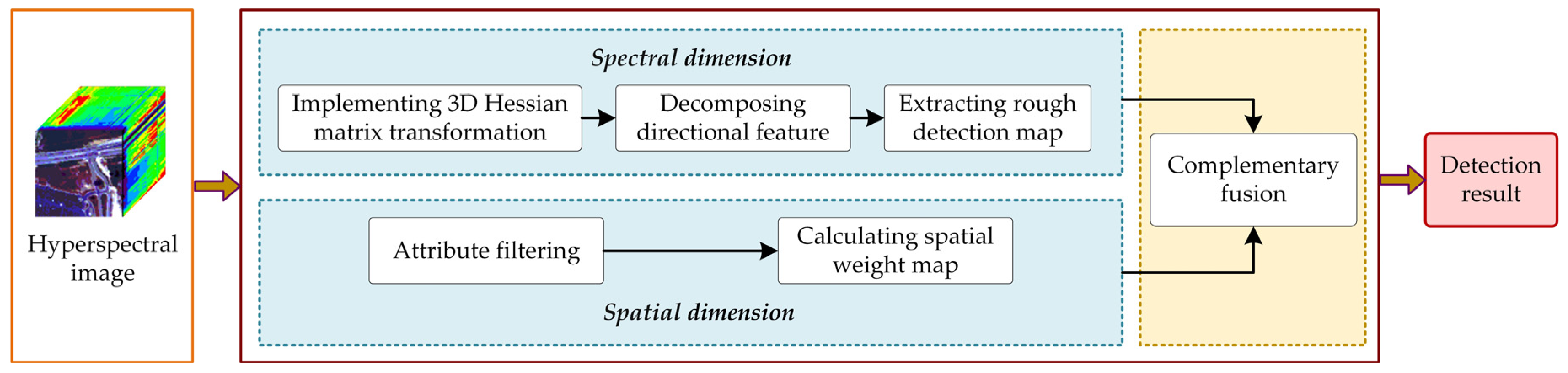
A spectral–spatial complementary decision fusion (SCDFSCDF) framework was constructed for hyperspectral anomaly detection. In the entire framework, the spectral features and spatial features were fused to ensure satisfactory detection results.
(2)
For the first time, because a three–dimensional Hessian matrix can exploit the spectral information and the three–dimensional spatial structure information of the HSI, it is introduced to hyperspectral anomaly detection to obtain the directional feature images, which can highlight the anomaly targets and suppress the background pixels in HSIs. The three–dimensional Hessian matrix not only contains the spectral information of the HSI, but also does not break the overall structural information of the HSI.
(3)
The truncated nuclear norm approximates the rank function more accurately by minimizing the sum of a few of the smallest singular values. Therefore, to more accurately separate the sparse matrix containing anomaly targets from the directional feature images, we exploited LRSMD with the truncated nuclear norm (TNN) and sparse regular terms for the first time in hyperspectral anomaly detection. In the LRSMD, TNN replaced the nuclear norm to better approximate the rank function. In addition, a sparse regular term of the l2,1–norm was added.
The rest of this paper is organized as follows. The proposed approach is described in detail in Section 2. The experimental datasets and the evaluation indicators are introduced in Section 3. The parameter analysis, the experimental results and the performance analysis of the proposed method are discussed in Section 4. In Section 5, the work is summarized.

2. Proposed Approach

This article combines the spectral–spatial features and proposes a hyperspectral anomaly detection method based on spectral–spatial complementary decision fusion. The processing of spectral–spatial features is regarded as completed in their respective dimensions. These dimensions are named the spectral dimension and spatial dimension, respectively. In this section, we describe this method in detail.

2.1. SCDF Framework

The proposed SCDF–based hyperspectral anomaly detection scheme is shown in Figure 1, which includes three parts: the spectral dimension, the spatial dimension and the result complementary fusion. In the spectral dimensions, three–directional feature images are extracted through the three–dimensional Hessian matrix. After that, the sparse matrices containing anomaly targets are obtained by executing LRSMD with the TNN and sparse regular terms on the three–directional feature images. Finally, the rough detection maps are extracted from the obtained sparse matrices. In the spatial dimension, the spatial feature of HSI is extracted through attribute filtering. Then, the spatial weight map is obtained from the spatial feature. In the complementary fusion of results, the final detection result is obtained by fusing the spatial weight map and the rough detection maps.

2.2. Spectral Dimension

The spectral dimension we named mainly includes the three–dimensional Hessian matrix of HSI, LRSMD–TNN, and the extraction of rough detection results.

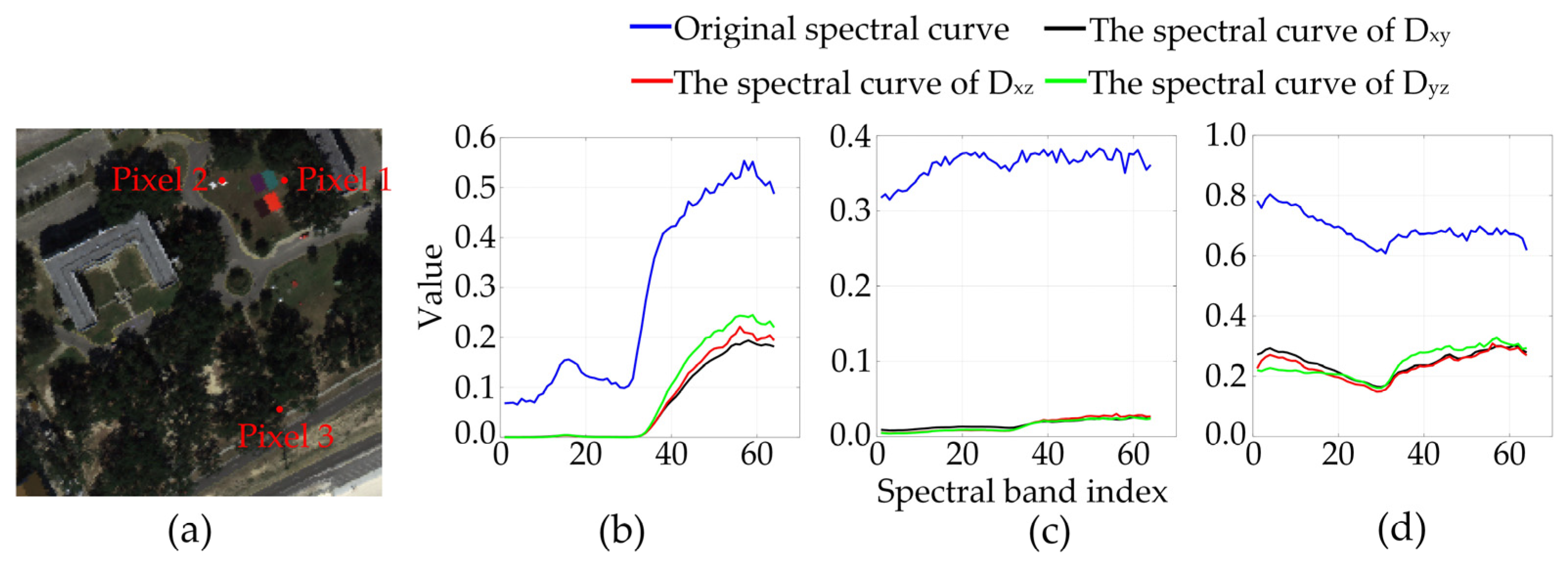
2.2.1. Three–Dimensional Hessian Matrix of the HSI

Anomalies usually only occupy a few pixels in the HSI and can be regarded as a small target area relative to the local homogeneous background. The determinant of the Hessian matrix can express the local structural features of the image [47,48,49]. It can be employed to highlight the target structure in the image and filter out other information. Therefore, the determinant of the Hessian matrix is used in anomaly detection to find the anomaly target structure in the HSI. Considering that the two–dimensional Hessian matrix does not exploit the spectral information and the three–dimensional spatial structure information of the HSI, the three-dimensional Hessian matrix is finally exploited.
The three–dimensional Hessian matrix of the HSI is actually used to obtain the second–order partial derivative of the HSI. Furthermore, according to the linear scale space theory [50], the derivative of a function is equal to the convolution of the function and the derivative of the Gaussian function. As such, only the second–order partial derivatives of the Gaussian function in each direction are required, then the second–order partial derivatives of the HSI in each direction can be obtained.
In the three–dimensional Hessian matrix, the Gaussian function can be represented as:
f ( x , y , z ) = ( 1 2 π σ ) 3 e x 2 + y 2 + z 2 2 σ 2 x , y , z W
where σ represents the standard deviation and W represents the size of the window as w × w × w. The x and y represent the two–dimensional spatial position coordinates of the HSI, respectively. The z represents the spectral dimension coordinate of the HSI. The second–order partial derivative 2 f ( x , y , z ) x 2 , 2 f ( x , y , z ) y 2 , 2 f ( x , y , z ) z 2 , 2 f ( x , y , z ) x y , 2 f ( x , y , z ) x z and 2 f ( x , y , z ) y z of the Gaussian function with respect to x, y, and z is shown as:
2 f x , y , z x 2 = 1 ( 2 π σ ) 3 x 2 σ 2 σ 4 e x 2 + y 2 + z 2 2 σ 2 = x 2 σ 2 ( 2 π ) 3 σ 7 e x 2 + y 2 + z 2 2 σ 2 2 f x , y , z y 2 = 1 ( 2 π σ ) 3 y 2 σ 2 σ 4 e x 2 + y 2 + z 2 2 σ 2 = y 2 σ 2 ( 2 π ) 3 σ 7 e x 2 + y 2 + z 2 2 σ 2 2 f x , y , z z 2 = 1 ( 2 π σ ) 3 z 2 σ 2 σ 4 e x 2 + y 2 + z 2 2 σ 2 = z 2 σ 2 ( 2 π ) 3 σ 7 e x 2 + y 2 + z 2 2 σ 2 2 f x , y , z x y = 1 ( 2 π σ ) 3 x y σ 4 e x 2 + y 2 + z 2 2 σ 2 = x y ( 2 π ) 3 σ 7 e x 2 + y 2 + z 2 2 σ 2 2 f x , y , z x z = 1 ( 2 π σ ) 3 x z σ 4 e x 2 + y 2 + z 2 2 σ 2 = x z ( 2 π ) 3 σ 7 e x 2 + y 2 + z 2 2 σ 2 2 f x , y , z y z = 1 ( 2 π σ ) 3 y z σ 4 e x 2 + y 2 + z 2 2 σ 2 = y z ( 2 π ) 3 σ 7 e x 2 + y 2 + z 2 2 σ 2
In this paper, HSI is represented by the bold letter H = (h1, h2, …, hm×n) Rm×n×b, where m × n represents the number of all pixels in the HSI, and b represents the number of bands of the HSI. The second–order partial derivatives Ixx, Iyy, Izz, Ixy, Ixz, and Iyz of the HSI H with respect to x, y, and z can be obtained by:
I x x = H x , y , z * 2 f x , y , z x 2 = H x , y , z * x 2 σ 2 ( 2 π ) 3 σ 7 e x 2 + y 2 + z 2 2 σ 2 I y y = H x , y , z * 2 f x , y , z y 2 = H x , y , z * y 2 σ 2 ( 2 π ) 3 σ 7 e x 2 + y 2 + z 2 2 σ 2 I z z = H x , y , z * 2 f x , y , z z 2 = H x , y , z * z 2 σ 2 ( 2 π ) 3 σ 7 e x 2 + y 2 + z 2 2 σ 2 I x y = H x , y , z * 2 f x , y , z x y = H x , y , z * x y ( 2 π ) 3 σ 7 e x 2 + y 2 + z 2 2 σ 2 I x z = H x , y , z * 2 f x , y , z x z = H x , y , z * x z ( 2 π ) 3 σ 7 e x 2 + y 2 + z 2 2 σ 2 I y z = H x , y , z * 2 f x , y , z y z = H x , y , z * y z ( 2 π ) 3 σ 7 e x 2 + y 2 + z 2 2 σ 2
where * is defined as a convolution operation. It is worth noting that the second–order partial derivatives of the HSI at (x, y, z) in the yx, zx, and zy directions are equal to the second–order partial derivatives in the xy, xz, and yz directions, respectively. Then, the determinant of the three–dimensional Hessian matrix in the xy, xz, and yz directions can be calculated by:
D x y = I x x I y y I x y I x y I x x I y y I x y I x y D x z = I x x I z z I x z I x z I x x I z z I x z I x z D y z = I y y I z z I y z I y z I y y I z z I y z I y z
where Dxy, Dxz and Dyz have the same size as the original HSI H, represents the matrix dot product. We employ the determinant in each direction to express the directional feature of the HSI.
Figure 2 shows the spectral curves before and after the transformation of the three–dimensional Hessian matrix of three random pixels in the MUUFL Gulfport HSI. As shown in Figure 2a, the covers corresponding to pixels 1 and 3 are two different mixed ground surfaces, respectively, and the cover corresponding to pixel 2 is a tree. It can be seen from Figure 2b–d that after the three–dimensional Hessian matrix transformation, the background is suppressed to a certain extent. The MUUFL Gulfport HSI is introduced in detail in Section 3.

2.2.2. LRSMD–TNN

After obtaining the directional feature images of the HSI, we performed the LRSMD on the directional feature images to obtain the sparse matrix containing anomaly targets. Each directional feature image needed to be transformed into a two–dimensional matrix D Rb×mn in advance, and then the LRSMD was performed. The typical LRSMD model [51] can be written as:
min L , S rank ( L ) + λ S 1 s . t . D = L + S
where D represents the matrix to be decomposed. L Rb×mn represents the decomposed low–rank matrix, which mainly contains background information. S Rb×mn represents the decomposed sparse matrix, which contains anomaly targets information. rank(·) represents the rank function, ‖S1 = ∑i,j|Si,j| represents the l1–norm and λ is a parameter that balances low–rank and sparse matrices. To solve problem (5), most existing hyperspectral anomaly detection based on LRSMD applies the nuclear norm to approximate the rank function. As such, the optimized LRSMD model can be written as:
min L , S L * + λ S | | 1 s . t . D = L + S
where ‖·‖ indicates the nuclear norm, which is equal to the sum of the singular values of the matrix.
Although the LRSMD method based on the nuclear norm has achieved satisfactory results in hyperspectral anomaly detection, the nuclear norm cannot accurately approximate the rank function [52]. Specifically, in the rank function, all non–zero singular values have the same contribution to the rank of the matrix. However, in the nuclear norm, when the sum of all singular values is minimized, each non–zero singular value has a different contribution to the rank of the matrix [35,52,53]. In addition, these methods do not consider the intrinsic sparsity property in the low–rank matrix [54,55,56]. These factors will cause the decomposition result of the LRSMD method based on the nuclear norm to be inaccurate to some extent. In order to obtain the more accurate decomposition results, the TNN can replace the nuclear norm to approximate the rank function. The truncated nuclear norm only minimizes the sum of a few of the smallest singular values, because the rank of the matrix only corresponds to the first few non–zero singular values, and large non–zero singular values contribute little to the rank of the matrix [57,58]. Simultaneously, an extra sparse regular term on the low–rank matrix formed by l2,1–norm is introduced to consider the sparsity of the low–rank matrix in an intermediate transform domain. The low–rank matrix is considered sparse in the intermediate transform domain. We assume that g(·) represents the transform operator that transforms into the intermediate transform domain. Moreover, we used the l2,1–norm instead of the l1–norm to make the columns of S tend to be sparse. Thus, in our method, the LRSMD model is:
min L , S L r + λ S 2 , 1 + β g ( L ) 2 , 1 s . t . D = L + S
where β is a parameter that balances the sparsity of the low–rank matrix in the intermediate transform domain. ‖Lr is the TNN of L. It is defined as the sum of the minimum of m and n minus the r minimum singular values of L. ‖·‖2,1 represents the l2,1–norm, which is defined as the sum of the l2–norm of each column in the matrix. g(·) represents the transform operator in the intermediate transform domain. Their specific form is as follows:
L r = o = r + 1 min ( m , n ) δ o
S 2 , 1 = i = 1 m n j = 1 b ( S j , i ) 2
where δo represents the o–th smallest singular value of L. Sj,i represents the element in the j–th row and i–th column of the matrix S. To solve Equation (7), a new two–stage iterative method [58] was adopted.
In the first stage, since solving Equation (7) is NP–hard, it cannot be solved directly. According to Theorem 1 in [58], suppose the singular value decomposition of D′ is:
D = U Σ V T
where U = (u1, u2, …, um) Rb×b, Σ Rb×mn and V = (v1, v2, …, vn) Rmn×mn. After taking out the first r singular values, we assume:
A = u 1 , u 2 ,   , u r T R r × b B = v 1 , v 2 ,   , v r T R r × m n
Then, we can obtain:
Tr ( A D B T ) = Tr ( ( u 1 , u 2 , , u r ) T U Σ V T ( v 1 , v 2 , , v r ) ) = Tr ( diag ( δ 1 , δ 2 , , δ r ) ) = o = 1 r δ o
where Tr(·) represents the trace of the matrix, and diag(·) stands for the diagonal matrix. Combined with Equation (12), the TNN is redefined as:
L r = o = r + 1 min ( m , n ) δ o = L * o = 1 r δ o = L * Tr ( A L B T )
Thus, the final optimized Equation (7) is as follows:
min L , S L * Tr ( A L B T ) + λ S 2 , 1 + β g ( L ) | | 2 , 1 s . t . D = L + S
Through iterative calculation of Equation (14), the final low–rank matrix L and sparse S can be obtained. Among them, since the low–rank matrix L is unknown, matrix D replaces the low–rank matrix L to calculate matrices A and B in each iteration. The iterative convergence condition is:
L t + 1 + S t + 1 D t F τ 1
where ‖·‖F represents the Frobenius norm of the matrix, τ1 is the reconstruction error, and t is the number of iterations.
In the second stage, to solve problem (14), it could first be divided into several sub–problems, and then we applied the idea of the alternating direction method of multipliers (ADMM) [59] to update each variable.
Since the transform operator g(L) in the intermediate transform domain of L is not conducive to function decoupling [60], we introduced the variable C, and let C = g(L). In addition, we assumed that At and Bt were obtained after the t–th iteration. Then, problem (14) can be redefined as:
min L , S L * T r ( A t L B t T ) + λ S | | 2 , 1 + β C | | 2 , 1 s . t . D = L + S C = g ( L )
The augmented Lagrangian function of problem (16) is expressed as:
£ ( L , S , C , X 1 , X 2 , μ ) = L * T r ( A t L B t T ) + λ S | | 2 , 1 + β C 2 , 1 + X 1 , D L S + X 2 , C g ( L ) + μ 2 ( D L S F 2 + C g ( L ) F 2 )
where X1 and X2 represent Lagrange multipliers. The penalty coefficient is represented by μ > 0. The inner product of the matrix is represented by , .
For the multivariate in problem (17), the alternate update method can be utilized. When we update a variable, we keep other variables unchanged. Therefore, problem (17) can be broken down into the following subproblems in the k–th iteration under the t–th iteration of the first stage.
When we keep S and C unchanged and update L, it is:
L k + 1 = arg min L L k * + μ k 2 D L k S k + A t T B t μ k + ( X 1 ) k μ K F 2 + μ k 2 C k g ( L k ) + ( X 2 ) k μ K F 2
In order to solve the problem of the transform operator g(·), combined with the theorem of Parseval [60] and Theorem 2 in [58], we know that the sum (or integral) of the squares of a function is equal to the sum (or integral) of the squares of its Fourier transform. For example, ξ F 2 = ζ F 2 , where ξ = χ ( ζ ) , and χ ( ) is a unitary transform. Hence, we suppose that g(·) is a unitary transform and G(·) is the inverse transform of g(·). By applying the inverse transform G(·) to problem (18), we can get:
L k + 1 = arg min L L k * + μ k L k 1 2 D S k + A t T B t + ( X 1 ) k μ k + G C k + ( X 2 ) k μ K F 2
Problem (19) can be solved using the classical singular value shrinkage operator. Then, the objective function can finally be written as:
L k + 1 = SVT 1 2 μ k 1 2 D S k + 1 μ k A t T B t + ( X 1 ) k + G C k + ( X 2 ) k μ k
where the definition of SVTδ(·) is as follows: when given a matrix Q and δ′ > 0, SVTδ(·) can be expressed as SVT   δ ( Q ) = U diag [ max ( ω   δ ) ] V T , U R m × r , V R r × n and ω = ( δ 1 , δ 2 , , δ r ) T is the first r singular values of the matrix Q.
When we keep L and C unchanged and update S, the objective function is:
S k + 1 = arg min S λ S k 2 , 1 + μ k 2 D S k L k + 1 + ( X 1 ) k μ k F 2
When we keep L and S unchanged and update C, the objective function is:
C k + 1 = arg min C β C 2 , 1 + μ k 2 C g ( L k + 1 ) + ( X 2 ) k μ k F 2
The updated method of Lagrange multipliers X1 and X2 is:
( X 1 ) k + 1 = ( X 1 ) k + μ k ( D L k + 1 S k + 1 ) ( X 2 ) k + 1 = ( X 2 ) k + μ k C k + 1 g ( L k + 1 )
The updated method of penalty coefficient μ is:
μ k + 1 = min ( ε μ k , μ max )
where ε > 1 is a given fixed value that is utilized to update the penalty coefficient μ. μmax is the maximum value of the given penalty coefficient μ.
The convergence condition is:
L k + 1 L k F τ 2   or   S k + 1 S k F τ 2
where τ2 is the reconstruction error.
The detailed solution method of the LRSMD–TNN is shown in Algorithm 1. After performing the LRSMD–TNN on the three–directional feature images Dxy, Dxz and Dyz, we can obtain the three corresponding sparse matrices Sl (l = 1, 2, 3).

2.2.3. The Extraction of Rough Detection Results

After obtaining the sparse matrix Sl, we extract the rough detection result through finding the Mahalanobis distance. For the measured pixel s i l in the sparse matrix Sl, the Mahalanobis distance is:
E l = ( s i l u g l ) T C g l ( s i l u g l ) , i = 1 , 2 , , m × n
where El is the rough detection map, u g l is the mean vector of the sparse matrix Sl and C g l is the covariance matrix of the sparse matrix Sl.
Algorithm 1 Low–rank and sparse matrix decomposition with truncated nuclear norm
Input: Directional feature image D.
Initialization: parameter λ > 0 and β > 0, number of singular values r < min(m,n), penalty coefficient μ0 and μmax, parameter ε > 1, reconstruction error τ1 and τ2, number of iterations t = k = 1, L1 = S1 = X1 = X1 = C1 = 0, D1 = D.
While Equation (15) does not converge do
      (1) Update At and Bt according to Equations (10) and (11).
      While Equation (25) does not converge do
        (2) Update Lk+1 according to Equation (20).
        (3) Update Sk+1 according to Equation (21).
        (4) Update Ck+1 according to Equation (22).
        (5) Update (X1)k+1 and (X2)k+1 according to Equation (23).
        (6) Update μk+1 according to Equation (24).
      End
      Return Lt+1, St+1 and Dt+1.
End
Return L and S.

2.3. Spatial Dimension

The above method mainly considers the spectral characteristics of anomaly targets in the HSI, but do not consider their spatial characteristics. In the spatial dimension, anomaly targets usually appear in the form of low probability and small area [61]. When the spectra of the anomaly targets are similar to those of the background, the spatial feature can be exploited to distinguish the anomaly targets from the background. At present, the anomaly detection based on attribute and edge–preserving filters (AED) [62] has achieved excellent results in extracting the spatial features of the HSI. The attribute filtering can remove the connected bright and dark part of the HSI. Therefore, we further combine the spatial characteristics of the HSI through the attribute filtering.
In this section, we perform attribute filtering and differential operation on each band of the original HSI to extract spatial feature image M Rm×n×b, which can be obtained by:
M j = H j A η ( H j ) + H j A θ ( H j )
where Mj (j = 1, 2, …, b) is the j–th band of the obtained spatial feature image M. Hj is the j–th band of the HSI, and Aη and Aθ represent attribute thinning and thickening performed on the regions with values greater than a given threshold and regions with values less than a given threshold in the HSI, respectively, which are described in detail in the background section of [55]. Through these two operations, the spatial features in the HSI can be preserved. Then, the spatial anomaly detection result T is obtained through the l2–norm, as shown below:
T ( i ) = j = 1 b ( m ^ j , i ) 2 , i = 1 , 2 , , m × n
where T(i) is the i–th pixel of the spatial anomaly detection result T, and m ^ j , i is the i–th pixel in the j–th band in the spatial feature image M. Since the spatial anomaly detection result T is used as the complementary fusion weight of the aforementioned rough detection map El, we named the spatial anomaly detection result as the spatial weight map.

2.4. Complementary Fusion

In the final result fusion stage, the final detection result is obtained by fusing each dimension detection result. The spatial features and spectral features can be further complemented through fusion. The specific operation is to merge the detection result of each spectral dimension with the detection result of the spatial dimension. This can ensure that the detection results of other dimensions are supplemented to a certain extent when the detection effect of a certain dimension is not satisfactory. In this way, the spectral characteristics and the spatial characteristics are complementary to achieve satisfactory results. Hence, the final detection map F is obtained by:
F = T l = 1 3 E l
where represents the matrix dot product.
Through the above methods, the spectral characteristics and spatial characteristics can be combined to obtain optimized detection results. The fusion method can further suppress background information, which is also verified by the experimental results. The detailed steps of the proposed SCDF method are shown in Algorithm 2.
Algorithm 2 Spectral–spatial complementary decision fusion
Input: HSI H.
Initialization: standard deviation σ, window size w, number of singular values r, predefined logical predicate Tρ.
      (1) Calculate the directional feature images Dxy, Dxz and Dyz by Equations (2)–(4).
      (2) Calculate the sparse matrix Sl by Algorithm 1.
      (3) Get the rough detection map El by Equation (26).
      (4) Extract the spatial feature image M by Equation (27).
      (5) Calculate the spatial weight map T by Equation (28).
      (6) Obtain the final detection map F by Equation (29).
Return the final detection map F.

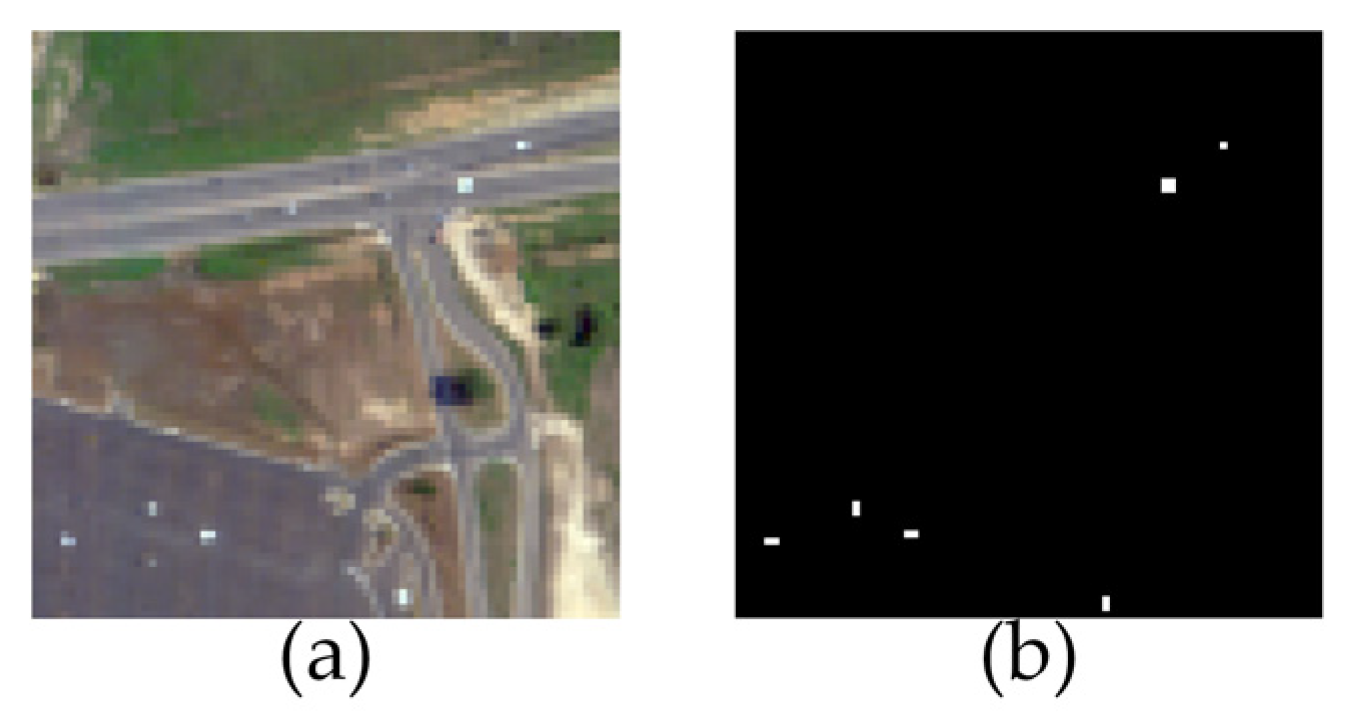
3. Experimental Dataset and Evaluation Indicator

In this section, we first discuss the synthetic and three real datasets in brief. Secondly, the evaluation indicators used in the experiments are introduced.

3.1. Experimental Dataset

Synthetic dataset: The synthetic data [63] are provided by Tan et al. The background of the synthetic dataset is cropped from the Salinas dataset, collected from Salinas Valley, CA, USA, by Airborne Visible/Infrared Imaging Spectrometer (AVIRIS). The Salinas dataset has a size of 512 × 217 and contains 224 bands. In the experiment, a 120 × 120 area was selected as the background of the synthetic data. In addition, after removing the water absorption and bad bands (108–112, 154–167 and 224), 204 bands were retained. The anomaly target is embedded in the background through the target implantation method.
z sp = f saf t ts + ( 1 f saf ) b bs
where zsp is the spectrum of the synthesized target, fsaf is the abundance fraction and bbs is the spectrum of the background. The range of fsaf is from 0.04 to 1. The synthetic data and the corresponding ground truth map are shown in Figure 3.
Urban: The second dataset was collected from an urban area by a hyperspectral digital imagery collection experiment (HYDICE) sensor [64]. The original dataset is a 400 × 400 HSI with a spatial resolution of 2 m per pixel. There are 210 bands in the original HSI. In our experiment, we cropped an 80 × 80 area, as shown in Figure 4a. After removing the water absorption bands and the low signal–to–noise ratio (SNR) bands (1–4, 76, 87, 101–111, 136–153, 198–210), 162 available bands were reserved. The corresponding ground truth map is shown in Figure 4b.
MUUFL Gulfport: The third dataset was collected from the University of Southern Mississippi Gulf Park Campus in Long Beach, Mississippi, USA, by the hyperspectral compact airborne spectrographic imager (CASI–1500) [65]. The original dataset is a 325 × 220 HSI. There are 72 bands in the original HSI. After the first four and last four noise bands are removed, the remaining 62 bands are reserved in the experiment. In our experiment, we crop a 200 × 200 area, as shown in Figure 5a. In this HSI, six cloth panels of different sizes are considered anomaly targets. The corresponding ground truth map is shown in Figure 5b.
Chikusei: The fourth dataset was acquired by Headwall Hyperspec–VNIR–C imaging sensor [66] in Chikusei, Ibaraki, Japan. The dataset contains 128 bands ranging from 363 nm to 1018 nm. The size of the original HSI with a spatial resolution of 2.5 m per pixel is 2517 × 2335. We cropped an area of 100 × 100 as the experimental image. All bands are included in the experiment. The corresponding ground truth map is made with the help of the Environment for Visualizing Images (ENVI) software. The false–color map of the Chikusei scene and the corresponding ground truth map are shown in Figure 6.

3.2. Evaluation Indicator

The alternative methods that we used in the experiment are the RX [15], the LRX [16], the LSMAD [30], the LSDM–MoG [32], the CDASC [21], the 2S–GLRT [20], the BFAD [44], the SSFSCRD [45], and the AED [62] methods. In the parameter analysis and discussion of experimental results, the three–dimensional receiver operating characteristic (3D ROC) [67] curve and the corresponding two–dimensional ROC (2D ROC) curves, and the area under the 2D ROC curve (AUC) are utilized as evaluation indicators to quantitatively evaluate the performance of the proposed method. With the same threshold τ, the 3D ROC curve (PD, PF, τ) can more accurately evaluate the performance of each method. PD is the probability of detection and PF is the false alarm probability. The corresponding 2D ROC curves are (PD, PF), (PD, τ), and (PF, τ). The AUC values of the three 2D ROC curves are AUC(D,F), AUC(D,τ), and AUC(F,τ). The AUC(D,F), AUC(D,τ), and AUC(F,τ) indicate the effectiveness, target detectability (TD), and background suppressibility (BS) of the detection method, respectively. In addition to these three AUC values, another five AUC values [63] are also proposed to evaluate the performance of the detection method. They are represented as AUCTD, AUCBS, AUCSNPR, AUCTDBS, and AUCODP, respectively. Among them, AUCTD calculates the effectiveness and TD of a detection method.
0 AUC TD = AUC ( D , F ) + AUC ( D , τ ) 2
By combining the BS of a detection method, AUCBS is defined as:
1 AUC BS = AUC ( D , F ) AUC ( F , τ ) 1
In order to comprehensively consider the TD and BS of a detection method, AUCTDBS is defined as:
1 AUC TDBS = AUC ( D , τ ) AUC ( F , τ ) 1
The signal–to–noise probability ratio AUCSNPR is defined as:
0 AUC SNPR = AUC ( D , τ ) AUC ( F , τ )
The overall detection probability AUCODP is defined as:
0 AUC TDBS = AUC ( D , F ) + AUC ( D , τ ) AUC ( F , τ ) 2
It is worth noting that the smaller the AUC(F,τ) value, the better the performance of the detection method. The larger the other AUC values, the better the performance of the detection method.

4. Discussion

In this section, the parameters of the proposed SCDF method are first analyzed in detail. Then, the effectiveness and superiority of the proposed SCDF method is demonstrated by qualitative and quantitative comparison with alternative methods. Finally, the dimension performance and the performance of TNN of the proposed SCDF method are analyzed and discussed.

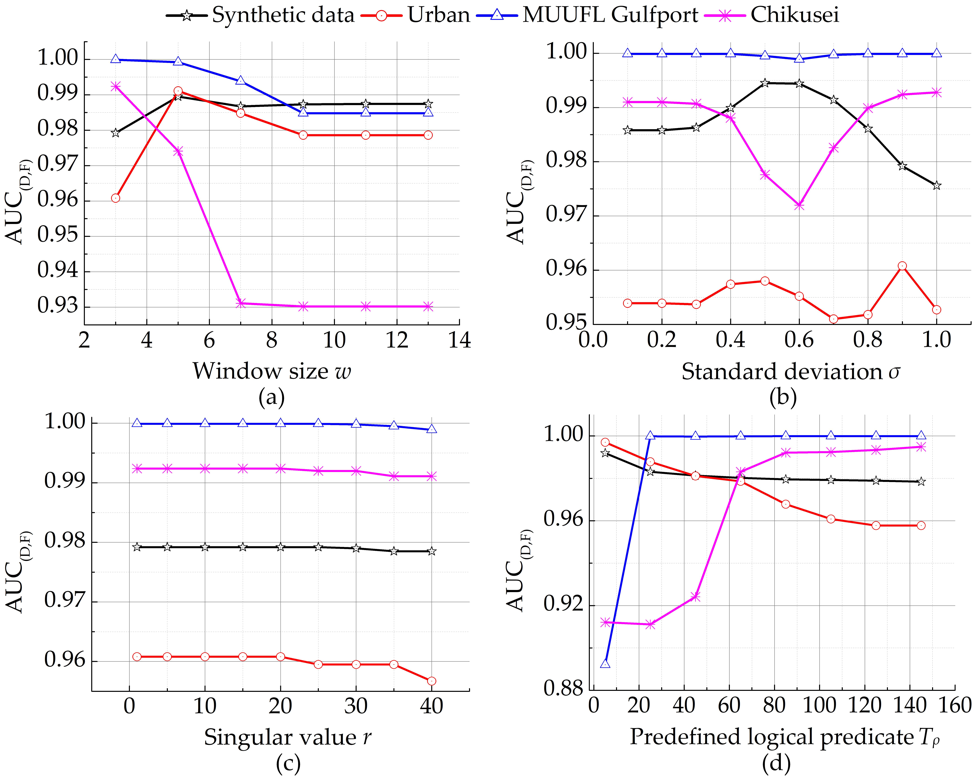
4.1. Parameter Analysis

In the experiment, the uncertain parameters in the alternative methods were selected according to the AUC(D,F) value or the parameter values provided by the original authors. On the four experimental datasets, the values of the uncertain parameters of all alternative methods are shown in Table 1.
The parameters of the proposed SCDF method were window size w, the standard deviation σ, parameters λ and β, number of singular values r, penalty coefficient μ0 and μmax, parameter ε, reconstruction errors τ1 and τ2, and the predefined logical predicate Tρ. Although there were many parameters in the proposed SCDF method, some parameters had little effect on the performance of the proposed method, such as penalty coefficient μ0 and μmax, parameter ε, and reconstruction errors τ1 and τ2. Therefore, we set μ0 = 0.005, μmax = 10,000, ε = 1.01, and τ1 = τ2 = 10−6. In addition, for the parameters λ and β, according to the recommendations of the previous studies and the analysis of experimental results [52,53,58], we finally set the two parameters to λ = 0.0005 and β = 0.00009. Consequently, the remaining uncertain parameters include window size w, the standard deviation σ, the number of singular values r, and the predefined logical predicate Tρ.
To determine the optimal values of these uncertain parameters, when analyzing one of the uncertain parameters of the proposed SCDF method in the experiment, the other parameters are kept constant. In the experiment, the AUC(D,F) value is used as the evaluation index. At the beginning of the experiment, the default parameters are set to w = 3, σ = 0.9, r = 20, and Tρ = 105. The analysis results of the impact of the four parameters on the performance of the proposed SCDF method are shown in Figure 7. These uncertain parameters are mainly determined according to the AUC(D,F) values in Figure 7. Finally, the window size w is set to w = 5 in the synthetic dataset and the urban dataset. In the MUUFL Gulfport dataset and the Chikusei dataset, w is set to w = 3. For the standard deviation σ, σ is set to σ = 0.9 in the urban dataset and the Chikusei dataset. In the synthetic dataset, σ is set to σ = 0.5. In the MUUFL Gulfport dataset, σ is set to σ = 1. In all datasets, the number of singular values r is uniformly set to r = 20. The predefined logical predicate Tρ, is set to Tρ = 5 in the synthetic dataset and the urban dataset, and Tρ = 145 in the Chikusei dataset and the MUUFL Gulfport dataset.

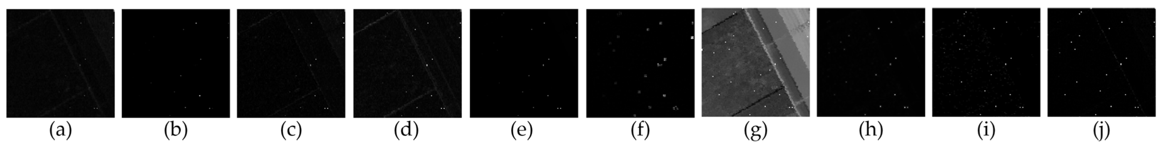
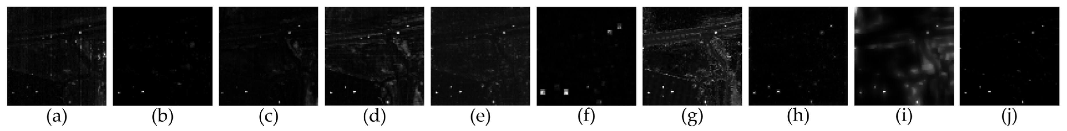
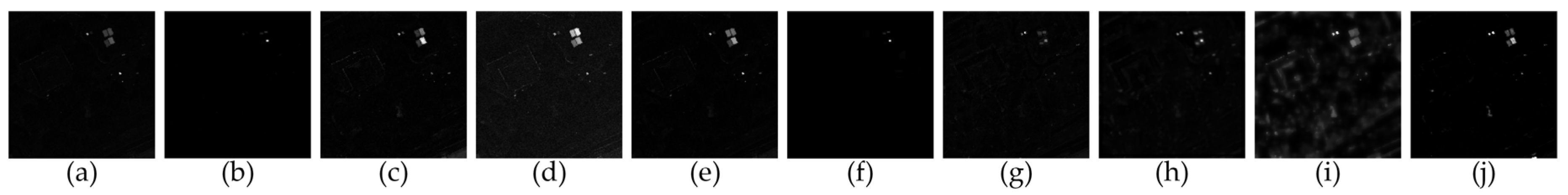
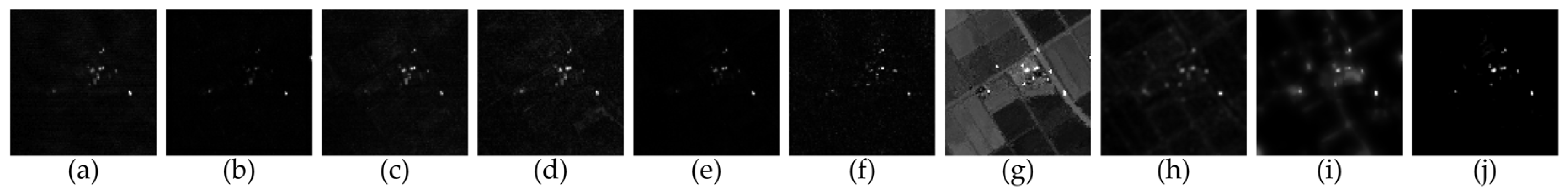
4.2. Experimental Results and Discussion

In the experiment, we evaluated the effectiveness and advancement of the proposed SCDF method from both visual detection effects and quantitative comparison. On different datasets, the detection results of the alternative methods and the proposed SCDF method are shown in Figure 8, Figure 9, Figure 10 and Figure 11.
It can be seen from Figure 8 that in addition to the BFAD method, other methods have better suppressed the background. In the detection results of the RX, the LRX, and the LSMAD methods, not all targets are well–separated from the background. The proposed SCDF method, as well as the LSDM–MoG, the CDASC, the 2S–GLRT, the BFAD, the SSFSCRD, and the AED methods can well–separate anomaly targets from the background. In addition, the anomaly targets in the detection results of the proposed SCDF method are more prominent.
As shown in Figure 9, on the urban dataset, the backgrounds of the detection results of the RX, the LSDM–MoG, and the BFAD methods are not well–suppressed. The background suppression effect is not very satisfactory in the detection result of the AED method. The detection results of other methods are relatively similar.
On the MUUFL Gulfport dataset, it can be seen from Figure 10 that all methods have detected anomaly targets, but they all contain a certain number of false targets. In the detection results of the LRX and the 2S–GLRT methods, the anomaly targets are not well–highlighted from the background. The detection results of the LSMAD, the LSDM–MoG, and the CDASC methods are similar to those of the proposed SCDF method. Among them, the targets in the detection results of the LSDM–MoG are relatively more obvious than the detection results of the proposed SCDF method, and the false alarms are slightly less. However, the proposed SCDF method still obtains satisfactory detection results.
Figure 11 shows the results of different methods on the Chikusei dataset. The detection results of the LRX, the CDASC, and the SSFSCRD methods are not particularly prominent. The background suppression is not particularly satisfactory in the detection results of the LSDM–MoG and the BFAD methods. The detection results of other methods are similar to those of the proposed SCDF method. It can be seen from the visual detection results of the four datasets that the proposed SCDF method obtains satisfactory detection results.
The 3D ROC curves and the corresponding 2D ROC curves of the detection results of different methods are shown in Figure 12, Figure 13, Figure 14 and Figure 15. The different AUC values calculated according to the 3D ROC curves on different datasets are shown in Table 2, Table 3, Table 4 and Table 5. First, on the synthetic dataset, Figure 12 shows that the 3D ROC curve of the proposed SCDF method is relatively close to those of most alternative methods, and the corresponding 2D ROC curves (PD, τ) and (PF, τ) can also draw similar conclusions. The corresponding 2D ROC curve (PD, PF) is slightly higher than those of other alternative methods. The corresponding AUC values are shown in Table 2. It can be seen from Table 2 that the AUC(D,F) and AUC(B,S) values of the proposed method are larger than those of the alternative methods, which are 0.9982 and 0.9976, respectively. Among the alternative and proposed methods, the AUC(F,τ) = 0.00008 and AUCSNPR = 3003.0358 of the LRX method are the largest, the AUC(D,τ) = 0.9340 and AUCTD = 1.8943 of the BFAD method are the largest, the AUCTDBS = 0.6755, and AUCODP = 1.6650 of the AED method are the largest. Although other AUC values do not reach the maximum values, they are still relatively close to the maximum AUC values. For example, AUC(F,τ) = 0.0005, AUCTD = 1.4833, AUCTDBS = 0.4845, and AUCODP = 1.4828 of the proposed SCDF method are close to the corresponding optimal AUC values of 0.00008, 1.8943, 0.6755, and 1.6650.
On the urban dataset, it can be seen from Figure 13 that the 3D ROC curve of the proposed SCDF method is higher than those of most alternative methods. The corresponding 2D ROC curves (PD, PF) are also very close to the 2D ROC curves of the BFAD and SSFSCRD methods. The 2D ROC curve (PD, τ) of the proposed SCDF method is slightly lower than those of the LSDM–MoG, the BFAD, and the CDASC methods. The 2D ROC curve (PF, τ) of the proposed SCDF method is lower than those of all alternative methods. Combining Table 3, we can see that the AUC(F,τ) = 0.0021, AUCBS = 0.9967 and AUCSNPR = 269.8049 of the proposed SCDF method are superior to all alternative methods. Among them, the AUC(D,τ) = 0.8330, AUCTD = 1.8290, AUCTDBS = 0.7474, and AUCODP = 1.7434 of the BFAD method are the largest among all methods. The AUC(D,F) = 0.9994 of the SSFSCRD method is the largest among all methods. However, the AUC values of the proposed SCDF method are also very close to the AUC values of the BFAD method. Therefore, the proposed SCDF method obtains a stable and excellent detection result on the urban dataset.
For the MUUFL Gulfport dataset, combining Figure 14 and Table 4, it can be seen that the comprehensive performance of the LSDM–MoG method is the best among the methods used in this work. The AUCBS = 0.9944 of the proposed SCDF method is better than those of the alternative methods. The AUC(D,F) = 0.9992, AUC(D,τ) = 0.6008, AUCTD = 1.6000, AUCTDBS = 0.5427, and AUCODP = 1.5419 of the LSDM–MoG method are the largest among all alternative and proposed methods. The AUC(F,τ) = 0.0003 and AUCSNPR = 135.2632 of the 2S–GLRT method are the largest among all alternative and proposed methods. Although the other AUC values of the proposed SCDF method are not the best, the difference between these AUC values and the optimal AUC values is very small. Therefore, the proposed SCDF method obtains an effective and stable detection result.
For the Chikusei dataset, it can be clearly seen from Figure 15 that the 2D ROC curves (PD, PF) and (PF, τ) are better than those of alternative methods. The 3D ROC curve and 2D ROC curve (PD, τ) of the BFAD method are superior to those of other methods. In Table 5, the AUC(D,F) = 0.9999, AUC(F,τ) = 0.0019, AUCBS = 0.9980, and AUCSNPR = 211.9936 of the proposed SCDF method are better than those of the alternative methods. However, the AUC(D,τ) = 0.8599, AUCTD = 1.8538, AUCTDBS = 0.6534, and AUCODP = 1.6474 of the BFAD method are superior to those of other alternative methods and the proposed SCDF method. On the Chikusei dataset, although the detection performance of the proposed SCDF method is not optimal in all aspects, it is also close to the detection performance of the BFAD method.

4.3. Complementary Dimension Performance Analysis

In this section, the complementary dimension performance of the proposed SCDF method is analyzed. The detection results of each dimension are compared with the final detection results from both qualitative and quantitative aspects. In the spectral dimension and the spatial dimension, the rough detection map and the spatial weight map are used as the dimension detection results, respectively. Figure 16 shows the visual detection results of each dimension and the final detection result. It can be clearly seen from Figure 16 that, compared to the detection results of each dimension, the background of the final detection result is cleaner and the anomaly targets of the final detection result are more prominent. In the final test results, there were fewer false alarms. As a consequence, from the visual effect analysis, the desired detection result is reached after the fusion. Additionally, it can be seen that when the detection result of a dimension is relatively poor, the remaining dimensions can be supplemented to obtain the desired detection result.
The AUC performance comparison corresponding to Figure 16 is shown in Table 6. It can be seen that on the synthetic dataset and the urban dataset, AUC(D,τ), AUCTD, AUCTDBS, and AUCODP values of the detection result of dimension 1 are the best. On the Chikusei dataset, AUC(D,F) = 0.9999, AUC(D,τ) = 0.6345, AUCTDBS = 0.6190, and the AUCODP = 1.6189 of the detection result of dimension 1 are the best. However, on the MUFL Gulfport dataset, the detection performance of dimension 1 is not the best. On the urban, MUFL Gulfport and Chikusei datasets, AUC(D,F), AUC(F,τ), AUCBS, and AUCSNPR values of the final detection results are the best. On the synthetic dataset, AUC(F,τ) = 0.0006, AUCBS = 0.9976 and AUCSNPR = 844.0422 of the final detection results are the best. Therefore, the final detection results are more satisfactory overall. At last, by combining Figure 16 and Table 6, we can conclude that the proposed SCDF method makes full use of the information of each dimension from the experimental results, thereby ensuring the superiority and effectiveness of the detection results.

4.4. The Performance Analysis of TNN

In order to verify the performance of TNN, we did not add the TNN in the LRSMD and still used the nuclear norm. We denoted the method of using the nuclear norm as SCDF–noTNN. The proposed method is denoted as SCDF–TNN. The AUC values were used as the evaluation index. The detection results of the two methods on the experimental datasets are shown in Figure 17. The corresponding AUC values are shown in Table 7. It can be seen from Figure 17 that the detection results of the two methods are very close. In Table 7, on the urban dataset, AUC(D,τ) = 0.6562, AUCTD = 1.6534, AUCTDBS = 0.6481 and AUCODP = 1.6453 of the SCDF–noTNN method are slightly larger than those of the SCDF–TNN method. On the MUUFL Gulfport dataset, AUC(F,τ) = 0.0004 of the SCDF–noTNN method is slightly smaller than that of the SCDF–TNN method. However, all the AUC values of the SCDF–TNN method on other datasets are larger than those of the SCDF–noTNN method. Although the improvement is slight, there is still a certain degree of improvement in the detection results of the SCDF–TNN method. In addition, it can be seen that the spectral–spatial complementary decision fusion framework that we proposed is helpful for anomaly detection. Therefore, it can be concluded that the proposed method in this paper is effective and competitive.

5. Conclusions

In this paper, we proposed a novel spectral–spatial complementary decision fusion method for hyperspectral anomaly detection. This proposed method is mainly divided into three parts: the spectral dimension, the spatial dimension, and the results fusion. First of all, in the spectral dimension, the three–dimensional Hessian matrix transformation was first introduced to obtain directional feature maps in hyperspectral anomaly detection. Next, LRSMD with TNN was first adopted to decompose the directional feature images to obtain the sparse matrix. Finally, the rough detection map is extracted from the sparse matrix by Mahalanobis distance. In the spatial dimension, attribute filtering is employed to extract the spatial features of the HSI as the complementary spatial weight map of the spectral features. In the decision fusion stage, the spatial weight map and the rough detection maps are fused together to obtain the final anomaly detection result. In this way, the proposed method makes full use of the complementary advantages of the spectral features and spatial features of HSI in each dimension. On the synthetic and real–world datasets, compared with other state–of–the–art comparative methods, experimental results show the advancement and superiority of the method proposed in this paper from qualitative and quantitative analysis.
Additionally, the uncertain parameters in the proposed SCDF method are not determined automatically. This limits the detection performance of the proposed method. Moreover, the proposed SCDF method does not consider the case of mixed pixels. In the future, we will mainly work on adaptive anomaly detection methods to improve the robustness of the anomaly detection methods. Furthermore, we will also consider the impact of mixed pixels on detection performance.

Author Contributions

Conceptualization, P.X. and J.Z.; methodology, P.X.; software, P.X. and J.S.; validation, H.L., D.W. and H.Z.; formal analysis, J.Z.; investigation, P.X. and H.L.; resources, H.Z.; data curation, J.Z., D.W. and H.L.; writing—original draft preparation, P.X. and J.Z.; writing—review and editing, H.L., J.S., D.W. and H.Z.; visualization, P.X. and H.L.; supervision, H.Z. and J.S.; funding acquisition, H.L. and J.S. All authors have read and agreed to the published version of the manuscript.

Funding

This research was funded by the Aeronautical Science Foundation of China under grant number 201901081002, the National Natural Science Foundation of China under grant number 51801142 and the Equipment Pre–research Key Laboratory Foundation under grant number 6142107200208.

Institutional Review Board Statement

Not applicable.

Informed Consent Statement

Not applicable.

Data Availability Statement

Acknowledgments

The authors gratefully acknowledge Space Application Laboratory, Department of Advanced Interdisciplinary Studies, the University of Tokyo and other researchers for providing the hyperspectral datasets.

Conflicts of Interest

The authors declare no conflict of interest.

References

  1. Zhao, G.; Li, F.; Zhang, X.; Laakso, K.; Chan, J.C.-W. Archetypal analysis and structured sparse representation for hyperspectral anomaly detection. Remote Sens. 2021, 13, 4102. [Google Scholar] [CrossRef]
  2. Tang, L.; Li, Z.; Wang, W.; Zhao, B.; Pan, Y.; Tian, Y. An efficient and robust framework for hyperspectral anomaly detection. Remote Sens. 2021, 13, 4247. [Google Scholar] [CrossRef]
  3. Liu, S.; Zhang, L.; Cen, Y.; Chen, L.; Wang, Y. A fast hyperspectral anomaly detection algorithm based on greedy bilateral smoothing and extended multi-attribute profile. Remote Sens. 2021, 13, 3954. [Google Scholar] [CrossRef]
  4. Zhu, X.; Cao, L.; Wang, S.; Gao, L.; Zhong, Y. Anomaly detection in airborne Fourier transform thermal infrared spectrometer images based on emissivity and a segmented low-rank prior. Remote Sens. 2021, 13, 754. [Google Scholar] [CrossRef]
  5. Das, S.; Bhattacharya, S.; Khatri, P.K. Feature extraction approach for quality assessment of remotely sensed hyperspectral images. J. Appl. Remote Sens. 2020, 14, 026514. [Google Scholar] [CrossRef]
  6. Wang, J.; Xia, Y.; Zhang, Y. Anomaly detection of hyperspectral image via tensor completion. IEEE Geosci. Remote Sens. Lett. 2021, 18, 1099–1103. [Google Scholar] [CrossRef]
  7. Li, Z.; He, F.; Hu, H.; Wang, F.; Yu, W. Random collective representation-based detector with multiple features for hyperspectral images. Remote Sens. 2021, 13, 721. [Google Scholar] [CrossRef]
  8. Xiang, P.; Song, J.; Li, H.; Gu, L.; Zhou, H. Hyperspectral anomaly detection with harmonic analysis and low-rank decomposition. Remote Sens. 2019, 11, 3028. [Google Scholar] [CrossRef] [Green Version]
  9. Farooq, S.; Govil, H. Mapping regolith and gossan for mineral exploration in the eastern Kumaon Himalaya, India using hyperion data and object oriented image classification. Adv. Space Res. 2014, 53, 1676–1685. [Google Scholar] [CrossRef]
  10. Moriya, É.A.S.; Imai, N.N.; Tommaselli, A.M.G.; Miyoshi, G.T. Mapping mosaic virus in sugarcane based on hyperspectral images. IEEE J. Sel. Top. Appl. Earth Observ. Remote Sens. 2017, 10, 740–748. [Google Scholar] [CrossRef]
  11. Ellis, R.J.; Scott, P.W. Evaluation of hyperspectral remote sensing as a means of environmental monitoring in the St. Austell China clay (kaolin) region, Cornwall, UK. Remote Sens. Environ. 2004, 93, 118–130. [Google Scholar] [CrossRef]
  12. Liang, J.; Zhou, J.; Tong, L.; Bai, X.; Wang, B. Material based salient object detection from hyperspectral images. Pattern Recogn. 2018, 76, 476–490. [Google Scholar] [CrossRef] [Green Version]
  13. Zhao, C.; Zhang, L. Spectral–spatial stacked autoencoders based on low-rank and sparse matrix decomposition for hyperspectral anomaly detection. Infrared Phys. Technol. 2018, 92, 166–176. [Google Scholar] [CrossRef]
  14. Zhang, L.; Zhao, C. A spectral-spatial method based on low-rank and sparse matrix decomposition for hyperspectral anomaly detection. Int. J. Remote Sens. 2017, 38, 4047–4068. [Google Scholar] [CrossRef]
  15. Reed, I.S.; Yu, X. Adaptive multiple-band CFAR detection of an optical pattern with unknown spectral distribution. IEEE Trans. Acoust. Speech Signal Process. 1990, 38, 1760–1770. [Google Scholar] [CrossRef]
  16. Matteoli, S.; Diani, M.; Theiler, J. An overview of background modeling for detection of targets and anomalies in hyperspectral remotely sensed imagery. IEEE J. Sel. Top. Appl. Earth Observ. Remote Sens. 2014, 7, 2317–2336. [Google Scholar] [CrossRef]
  17. Guo, Q.; Zhang, B.; Ran, Q.; Gao, L.; Li, J.; Plaza, A. Weighted-RXD and linear filter-based RXD: Improving background statistics estimation for anomaly detection in hyperspectral imagery. IEEE J. Sel. Top/ Appl. Earth Observ. Remote Sens. 2014, 7, 2351–2366. [Google Scholar] [CrossRef]
  18. Carlotto, M.J. A cluster-based approach for detecting man-made objects and changes in imagery. IEEE Trans. Geosci. Remote Sens. 2005, 43, 374–384. [Google Scholar] [CrossRef]
  19. Tao, R.; Zhao, X.; Li, W.; Li, H.C.; Du, Q. Hyperspectral anomaly detection by fractional Fourier entropy. IEEE J. Sel. Top. Appl. Earth Observ. Remote Sens. 2019, 12, 4920–4929. [Google Scholar] [CrossRef]
  20. Liu, J.; Hou, Z.; Li, W.; Tao, R.; Orlando, D.; Li, H. Multipixel anomaly detection with unknown patterns for hyperspectral imagery. IEEE Trans. Neural Netw. Learn. Syst. 2021, 1–11. [Google Scholar] [CrossRef]
  21. Chen, S.; Chang, C.I.; Li, X. Component decomposition analysis for hyperspectral anomaly detection. IEEE Trans. Geosci. Remote Sens. 2022, 60, 5516222. [Google Scholar] [CrossRef]
  22. Tu, B.; Yang, X.; Ou, X.; Zhang, G.; Li, J.; Plaza, A. Ensemble entropy metric for hyperspectral anomaly detection. IEEE Trans. Geosci. Remote Sens. 2022, 60, 5513617. [Google Scholar] [CrossRef]
  23. Kwon, H.; Nasrabadi, N.M. Kernel RX-algorithm: A nonlinear anomaly detector for hyperspectral imagery. IEEE Trans. Geosci. Remote Sens. 2005, 43, 388–397. [Google Scholar] [CrossRef]
  24. Zhou, J.; Kwan, C.; Ayhan, B.; Eismann, M.T. A novel cluster kernel RX algorithm for anomaly and change detection using hyperspectral images. IEEE Trans. Geosci. Remote Sens. 2016, 54, 6497–6504. [Google Scholar] [CrossRef]
  25. Xie, W.; Jiang, T.; Li, Y.; Jia, X.; Lei, J. Structure tensor and guided filtering-based algorithm for hyperspectral anomaly detection. IEEE Trans. Geosci. Remote Sens. 2019, 57, 4218–4230. [Google Scholar] [CrossRef]
  26. Xing, C.; Wang, M.; Dong, C.; Duan, C.; Wang, Z. Joint sparse-collaborative representation to fuse hyperspectral and multispectral images. Signal Process. 2020, 173, 107585. [Google Scholar] [CrossRef]
  27. Wang, X.; Zhong, Y.; Cui, C.; Zhang, L.; Xu, Y. Autonomous endmember detection via an abundance anomaly guided saliency prior for hyperspectral imagery. IEEE Trans. Geosci. Remote Sens. 2021, 59, 2336–2351. [Google Scholar] [CrossRef]
  28. Chen, Y.; Nasrabadi, N.M.; Tran, T.D. Sparse representation for target detection in hyperspectral imagery. IEEE J. Sel. Top. Signal Process. 2011, 5, 629–640. [Google Scholar] [CrossRef]
  29. Li, W.; Du, Q. Collaborative representation for hyperspectral anomaly detection. IEEE Trans. Geosci. Remote Sens. 2015, 53, 1463–1474. [Google Scholar] [CrossRef]
  30. Zhang, Y.; Du, B.; Zhang, L.; Wang, S. A low-rank and sparse matrix decomposition-based Mahalanobis distance method for hyperspectral anomaly detection. IEEE Trans. Geosci. Remote Sens. 2016, 54, 1376–1389. [Google Scholar] [CrossRef]
  31. Xu, Y.; Wu, Z.; Li, J.; Plaza, A.; Wei, Z. Anomaly detection in hyperspectral images based on low-rank and sparse representation. IEEE Trans. Geosci. Remote Sens. 2016, 54, 1990–2000. [Google Scholar] [CrossRef]
  32. Li, L.; Li, W.; Du, Q.; Tao, R. Low-rank and sparse decomposition with mixture of gaussian for hyperspectral anomaly detection. IEEE Trans. Cybern. 2021, 51, 4363–4372. [Google Scholar] [CrossRef] [PubMed]
  33. Ma, Y.; Fan, G.; Jin, Q.; Huang, J.; Mei, X.; Ma, J. Hyperspectral anomaly detection via integration of feature extraction and background purification. IEEE Geosci. Remote Sens. Lett. 2021, 18, 1436–1440. [Google Scholar] [CrossRef]
  34. Qu, Y.; Wang, W.; Guo, R.; Ayhan, B.; Kwan, C.; Vance, S.; Qi, H. Hyperspectral anomaly detection through spectral unmixing and dictionary-based low-rank decomposition. IEEE Trans. Geosci. Remote Sens. 2018, 56, 4391–4405. [Google Scholar] [CrossRef]
  35. Li, L.; Li, W.; Qu, Y.; Zhao, C.; Tao, R.; Du, Q. Prior-based tensor approximation for anomaly detection in hyperspectral imagery. IEEE Trans. Neural Netw. Learn. Syst. 2022, 1–14. [Google Scholar] [CrossRef]
  36. Cheng, T.; Wang, B. Graph and total variation regularized low-rank representation for hyperspectral anomaly detection. IEEE Trans. Geosci. Remote Sens. 2020, 58, 391–406. [Google Scholar] [CrossRef]
  37. Nassif, A.B.; Talib, M.A.; Nasir, Q.; Dakalbab, F.M. Machine learning for anomaly detection: A systematic review. IEEE Access. 2021, 9, 78658–78700. [Google Scholar] [CrossRef]
  38. Racetin, I.; Krtali, A. Systematic review of anomaly detection in hyperspectral remote sensing applications. Appl. Sci. 2021, 11, 4878. [Google Scholar] [CrossRef]
  39. Xiang, P.; Zhou, H.; Li, H.; Song, S.; Tan, W.; Song, J.; Gu, L. Hyperspectral anomaly detection by local joint subspace process and support vector machine. Int. J. Remote Sens. 2020, 41, 3798–3819. [Google Scholar] [CrossRef]
  40. Xie, W.; Li, Y.; Lei, J.; Yang, J.; Chang, C.; Li, Z. Hyperspectral band selection for spectral-spatial anomaly detection. IEEE Trans. Geosci. Remote Sens. 2020, 58, 3426–3436. [Google Scholar] [CrossRef]
  41. Du, B.; Zhao, R.; Zhang, L.; Zhang, L. A spectral-spatial based local summation anomaly detection method for hyperspectral images. Signal Process. 2016, 124, 115–131. [Google Scholar] [CrossRef]
  42. Zhang, X.; Wen, G.; Dai, W. A tensor decomposition-based anomaly detection algorithm for hyperspectral image. IEEE Trans. Geosci. Remote Sens. 2016, 54, 5801–5820. [Google Scholar] [CrossRef]
  43. Lei, J.; Xie, W.; Yang, J.; Li, Y.; Chang, C.I. Spectral-spatial feature extraction for hyperspectral anomaly detection. IEEE Trans. Geosci. Remote Sens. 2019, 57, 8131–8143. [Google Scholar] [CrossRef]
  44. Yao, X.; Zhao, C. Hyperspectral anomaly detection based on the bilateral filter. Infrared Phys. Technol. 2018, 92, 144–153. [Google Scholar] [CrossRef]
  45. Zhao, C.; Li, C.; Feng, S.; Su, N.; Li, W. A spectral-spatial anomaly target detection method based on fractional Fourier transform and saliency weighted collaborative representation for hyperspectral images. IEEE J. Sel. Topics Appl. Earth Observ. Remote Sens. 2020, 13, 5982–5997. [Google Scholar] [CrossRef]
  46. Lu, X.; Zhang, W.; Huang, J. Exploiting embedding manifold of autoencoders for hyperspectral anomaly detection. IEEE Trans. Geosci. Remote Sens. 2020, 58, 1527–1537. [Google Scholar] [CrossRef]
  47. Lindeberg, T. Feature detection with automatic scale selection. Int. J. Comput. Vis. 1998, 30, 79–116. [Google Scholar] [CrossRef]
  48. Su, P.; Liu, D.; Li, X.; Liu, Z. A saliency-based band selection approach for hyperspectral imagery inspired by scale selection. IEEE Geosci. Remote Sens. Lett. 2018, 15, 572–576. [Google Scholar] [CrossRef]
  49. Du, Y.P.; Parker, D.L. Vessel enhancement filtering in three-dimensional MR angiograms using long-range signal correlation. J. Magn. Reson. Imaging 1997, 7, 447–450. [Google Scholar] [CrossRef]
  50. Skurikhin, A.N.; Garrity, S.R.; McDowell, N.G.; Cai, D.M.M. Automated tree crown detection and size estimation using multi-scale analysis of high-resolution satellite imagery. Remote Sens. Lett. 2013, 4, 465–474. [Google Scholar] [CrossRef]
  51. Sun, W.; Liu, C.; Li, J.; Lai, Y.M.; Li, W. Low-rank and sparse matrix decomposition-based anomaly detection for hyperspectral imagery. J. Appl. Remote Sens. 2014, 8, 083641. [Google Scholar] [CrossRef]
  52. Hu, Y.; Zhang, D.; Ye, J.; Li, X.; He, X. Fast and accurate matrix completion via truncated nuclear norm regularization. IEEE Trans. Pattern Anal. Mach. Intell. 2013, 35, 2117–2130. [Google Scholar] [CrossRef]
  53. Cao, F.; Chen, J.; Ye, H.; Zhao, J.; Zhou, Z. Recovering low-rank and sparse matrix based on the truncated nuclear norm. Neural Netw. 2017, 85, 10–20. [Google Scholar] [CrossRef]
  54. Gai, S. Color image denoising via monogenic matrix-based sparse representation. Vis. Comput. 2019, 35, 109–122. [Google Scholar] [CrossRef]
  55. Wright, J.; Yi, M.; Mairal, J.; Sapiro, G.; Huang, T.S.; Yan, S. Sparse representation for computer vision and pattern recognition. Proc. IEEE 2010, 98, 1031–1044. [Google Scholar] [CrossRef] [Green Version]
  56. Yang, J.; Wright, J.; Huang, T.S.; Ma, Y. Image super-resolution via sparse representation. IEEE Trans. Image Process. 2010, 19, 2861–2873. [Google Scholar] [CrossRef]
  57. Zhang, D.; Hu, Y.; Ye, J.; Li, X.; He, X. Matrix completion by truncated nuclear norm regularization. In Proceedings of the 2012 IEEE Conference on Computer Vision and Pattern Recognition, Providence, RI, USA, 16–21 June 2012; pp. 2192–2199. [Google Scholar]
  58. Xue, Z.; Dong, J.; Zhao, Y.; Liu, C.; Chellali, R. Low-rank and sparse matrix decomposition via the truncated nuclear norm and a sparse regularizer. Vis. Comput. 2019, 35, 1549–1566. [Google Scholar] [CrossRef]
  59. Kong, W.; Song, Y.; Liu, J. Hyperspectral image denoising via framelet transformation based three-modal tensor nuclear norm. Remote Sens. 2021, 13, 3829. [Google Scholar] [CrossRef]
  60. Merhav, N.; Kresch, R. Approximate convolution using DCT coefficient multipliers. IEEE Trans. Circuits Syst. Video Technol. 1998, 8, 378–385. [Google Scholar] [CrossRef]
  61. Andika, F.; Rizkinia, M.; Okuda, M. A hyperspectral anomaly detection algorithm based on morphological profile and attribute filter with band selection and automatic determination of maximum area. Remote Sens. 2020, 12, 3387. [Google Scholar] [CrossRef]
  62. Kang, X.; Zhang, X.; Li, S.; Li, K.; Li, J.; Benediktsson, J.A. Hyperspectral anomaly detection with attribute and edge-preserving filters. IEEE Trans. Geosci. Remote Sens. 2017, 55, 5600–5611. [Google Scholar] [CrossRef]
  63. Tan, K.; Hou, Z.; Wu, F.; Du, Q.; Chen, Y. Anomaly detection for hyperspectral imagery based on the regularized subspace method and collaborative representation. Remote Sens. 2019, 11, 1318. [Google Scholar] [CrossRef] [Green Version]
  64. Zhu, L.; Wen, G.; Qiu, S. Low-rank and sparse matrix decomposition with cluster weighting for hyperspectral anomaly detection. Remote Sens. 2018, 10, 707. [Google Scholar] [CrossRef] [Green Version]
  65. Du, X.; Zare, A. Technical Report: Scene Label Ground Truth Map for MUUFL Gulfport Data Set; Tech. Rep. 20170417; University of Florida Technical Report: Gainesville, FL, USA, 2017. [Google Scholar]
  66. Yokoya, N.; Iwasaki, A. Airborne hyperspectral data over Chikusei. Space Appl. Lab. Univ. Tokyo Jpn. 2016, SAL-2016-05-27, 1–6. [Google Scholar]
  67. Chang, C.I. An effective evaluation tool for hyperspectral target detection: 3d receiver operating characteristic curve analysis. IEEE Trans. Geosci. Remote Sens. 2021, 59, 5131–5153. [Google Scholar] [CrossRef]
Figure 1. Schematic of the proposed spectral–spatial complementary decision fusion for hyperspectral anomaly detection.
Remotesensing 14 00943 g001
Figure 2. The spectral curves before and after the transformation of the three–dimensional Hessian matrix of three random pixels in the MUUFL Gulfport HSI: (a) three pixels selected in the MUUFL Gulfport HSI; (b) the spectral curve of pixel 1 before and after the transformation of the three–dimensional Hessian matrix; (c) the spectral curve of pixel 2 before and after the transformation of the three–dimensional Hessian matrix; (d) the spectral curve of pixel 3 before and after the transformation of the three–dimensional Hessian matrix.
Remotesensing 14 00943 g002
Figure 3. Synthetic dataset: (a) false–color map of the synthetic dataset; (b) ground truth map of the synthetic dataset.
Remotesensing 14 00943 g003
Figure 4. Urban dataset: (a) false–color map of the urban dataset; (b) ground truth map.
Remotesensing 14 00943 g004
Figure 5. MUUFL Gulfport dataset: (a) false–color map of the MUUFL Gulfport dataset; (b) ground truth map.
Remotesensing 14 00943 g005
Figure 6. Chikusei dataset: (a) false–color map of the Chikusei dataset; (b) ground truth map.
Remotesensing 14 00943 g006
Figure 7. The influence of different parameters on the detection performance of the proposed method: (a) window size w; (b) standard deviation σ; (c) singular values r; (d) predefined logical predicate Tρ.
Remotesensing 14 00943 g007
Figure 8. The detection results of different methods on the synthetic dataset: (a) RX; (b) LRX; (c) LSMAD; (d) LSDM–MoG; (e) CDASC; (f) 2S–GLRT; (g) BFAD; (h) SSFSCRD; (i) AED; (j) SCDF.
Remotesensing 14 00943 g008
Figure 9. The detection results of different methods on the urban dataset: (a) RX; (b) LRX; (c) LSMAD; (d) LSDM–MoG; (e) CDASC; (f) 2S–GLRT; (g) BFAD; (h) SSFSCRD; (i) AED; (j) SCDF.
Remotesensing 14 00943 g009
Figure 10. The detection results of different methods on the MUUFL Gulfport dataset: (a) RX; (b) LRX; (c) LSMAD; (d) LSDM–MoG; (e) CDASC; (f) 2S–GLRT; (g) BFAD; (h) SSFSCRD; (i) AED; (j) SCDF.
Remotesensing 14 00943 g010
Figure 11. The detection results of different methods on the Chikusei dataset: (a) RX; (b) LRX; (c) LSMAD; (d) LSDM–MoG; (e) CDASC; (f) 2S–GLRT; (g) BFAD; (h) SSFSCRD; (i) AED; (j) SCDF.
Remotesensing 14 00943 g011
Figure 12. The 3D ROC curve and corresponding 2D ROC curves of different methods on the synthetic dataset: (a) 3D ROC curve; (b) corresponding 2D ROC curve (PD, PF); (c) corresponding 2D ROC curve (PD, τ); (d) corresponding 2D ROC curve (PF, τ).
Remotesensing 14 00943 g012
Figure 13. The 3D ROC curve and corresponding 2D ROC curves of different methods on the urban dataset: (a) 3D ROC curve; (b) corresponding 2D ROC curve (PD, PF); (c) corresponding 2D ROC curve (PD, τ); (d) corresponding 2D ROC curve (PF, τ).
Remotesensing 14 00943 g013
Figure 14. The 3D ROC curve and corresponding 2D ROC curves of different methods on the MUUFL Gulfport dataset: (a) 3D ROC curve; (b) corresponding 2D ROC curve (PD, PF); (c) corresponding 2D ROC curve (PD, τ); (d) corresponding 2D ROC curve (PF, τ).
Remotesensing 14 00943 g014
Figure 15. The 3D ROC curve and corresponding 2D ROC curves of different methods on the Chikusei dataset: (a) 3D ROC curve; (b) corresponding 2D ROC curve (PD, PF); (c) corresponding 2D ROC curve (PD, τ); (d) corresponding 2D ROC curve (PF, τ).
Remotesensing 14 00943 g015
Figure 16. Detection results of different dimensions. Each row represents the detection results of different dimensions on a dataset. Each column represents the detection results of the same dimension on different datasets: (a) synthetic dataset; (b) urban dataset; (c) MUUFL Gulfport dataset; (d) Chikusei dataset; (I) dimension 1; (II) dimension 2; (III) dimension 3; (IV) dimension 4; (V) final results.
Remotesensing 14 00943 g016
Figure 17. The detection results of the SCDF method with TNN and the SCDF method without TNN on each dataset: (a) SCDF–noTNN; (b) SCDF–TNN.
Remotesensing 14 00943 g017
Table 1. Uncertain parameter settings for different alternative methods on four datasets.
MethodParameter Setting
LRXThe size of window: (3, 5), (11, 15), (13, 31), (13, 15)
LSMADThe rank: 5, 6, 6, 30
The cardinality: 10, 1, 1, 5
LSDM–MoGThe rank: 60, 60, 30, 60
The number of mixture Gaussian noise: 4, 4, 4, 4
CDASCThe value of virtual dimensionality: 13, 10, 15, 10
The number of principal components: 2, 4, 6, 7
The number of independent components: 11, 6, 9, 3
2S–GLRTThe size of window: (3, 5), (5, 7), (13, 25), (5, 7)
BFADThe size of window: (3, 5), (3, 5), (13, 31), (5, 7)
The outputting sensitivity of spatial distance weight: 0.8, 5, 10, 0.5
The outputting sensitivity of spectral distance weight: 0.3, 1, 1, 0.3
SSFSCRDThe size of window: (3, 5), (5, 7), (13, 21), (3, 5)
The fractional order: 0.8, 0.5, 0.8, 0.9
The Lagrange multiplier: 0.5, 1, 0.1, 0.1
The weighting coefficient: 0.5, 0.1, 0.1, 0.1
AEDThe band number: 3, 3, 3, 3
The thresholding number: 5, 25, 125, 25
The domain transform recursive filtering: (1, 0.1). (5, 1), (5, 1), (5, 1)
Table 2. Comparison of AUC performance of different methods on the synthetic dataset.
MethodAUC(D,F)AUC(D,τ)AUC(F,τ)AUCTDAUCBSAUCSNPRAUCTDBSAUCODP
RX0.80730.21430.03141.02160.77596.83180.18290.9903
LRX0.98950.24140.000081.23090.98943003.03580.24131.2309
LSMAD0.89110.36400.01911.25510.872019.05360.34491.2360
LSDM–MoG0.97130.52050.03421.49180.937015.21350.48631.4576
CDASC0.99190.37250.00131.36440.9906280.91930.37121.3631
2S–GLRT0.94910.17440.00491.12350.944135.36080.16951.1185
BFAD0.96030.93400.29101.89430.66933.20930.64301.6033
SSFSCRD0.99160.47130.00831.46290.983356.86260.46301.4546
AED0.98950.67850.00301.66800.9865226.39400.67551.6650
SCDF0.99820.48510.00051.48330.9976844.04220.48451.4828
Table 3. Comparison of AUC performance of different methods on the urban dataset.
MethodAUC(D,F)AUC(D,τ)AUC(F,τ)AUCTDAUCBSAUCSNPRAUCTDBSAUCODP
RX0.96280.38590.05091.34870.91207.58570.33501.2978
LRX0.98120.25820.00751.23950.973834.50670.25071.2320
LSMAD0.27880.01720.03400.29600.24480.5068−0.01680.2620
LSDM–MoG0.99560.73600.05661.73170.939113.01270.67951.6751
CDASC0.98930.59170.06411.58110.92529.23150.52761.5170
2S–GLRT0.99220.31690.00971.30910.982432.54070.30721.2994
BFAD0.99600.83300.08561.82900.91049.73690.74741.7434
SSFSCRD0.99940.45560.00861.45500.990853.06100.44711.4465
AED0.99590.54540.06291.54130.93318.67530.48251.4784
SCDF0.99880.57910.00211.57790.9967269.80490.57691.5758
Table 4. Comparison of AUC performance of different methods on the MUUFL Gulfport dataset.
MethodAUC(D,F)AUC(D,τ)AUC(F,τ)AUCTDAUCBSAUCSNPRAUCTDBSAUCODP
RX0.99780.22470.01621.22250.981613.86120.20851.2063
LRX0.98400.04420.00101.02820.983045.16250.04331.0272
LSMAD0.99230.27350.01701.26580.975316.07250.25651.2488
LSDM–MoG0.99920.60080.05811.60000.941110.33780.54271.5419
CDASC0.99850.36610.01231.36460.986229.82520.35391.3524
2S–GLRT0.97020.04050.00031.01070.9699135.26320.04021.0104
BFAD0.94590.10920.01841.05510.92755.93320.09081.0367
SSFSCRD0.98650.16050.01811.14690.96848.88500.14241.1289
AED0.99190.29470.04861.28660.94336.06140.24611.2380
SCDF0.99490.04200.00051.03680.994484.74530.04151.0363
Table 5. Comparison of AUC performance of different methods on the Chikusei dataset.
MethodAUC(D,F)AUC(D,τ)AUC(F,τ)AUCTDAUCBSAUCSNPRAUCTDBSAUCODP
RX0.99910.33060.03371.32970.96549.81660.29691.2960
LRX0.98860.13960.00791.12820.980717.57290.13171.1203
LSMAD0.99850.26450.02811.26290.97049.42730.23641.2349
LSDM–MoG0.99290.41630.04111.40920.951810.13630.37521.3681
CDASC0.99960.21900.00521.21860.994442.05350.21371.2134
2S–GLRT0.98690.21920.01511.20610.971814.53010.20411.1910
BFAD0.99390.85990.20641.85380.78754.16510.65341.6474
SSFSCRD0.99770.33000.04091.32780.95688.06820.28911.2869
AED0.99720.48200.03531.47920.961913.65840.44671.4439
SCDF0.99990.40600.00191.40590.9980211.99360.40411.4041
Table 6. Comparison of AUC performance of different dimensions on various datasets.
DatasetDimensionAUC(D,F)AUC(D,τ)AUC(F,τ)AUCTDAUCBSAUCSNPRAUCTDBSAUCODP
Synthetic dataDimension 10.99050.70970.03001.70020.960523.68930.67971.6702
Dimension 20.97210.49550.03071.46760.941316.12210.46481.4368
Dimension 30.96720.49520.02511.46240.942119.71530.47001.4373
Dimension 40.99970.69060.02321.69030.976529.77630.66741.6671
Final result0.99820.48510.00061.48330.9976844.04220.48451.4828
UrbanDimension 10.99300.72490.03951.71790.953418.33030.68541.6783
Dimension 20.97710.57810.05271.55520.924410.96080.52531.5024
Dimension 30.99140.66120.06661.65260.92489.92580.59461.5859
Dimension 40.99820.70680.02711.70500.971226.11430.67971.6780
Final result0.99880.57910.00211.57790.9967269.80490.57691.5758
MUUFL GulfportDimension 10.99030.07370.00271.06400.987627.66080.07101.0613
Dimension 20.98960.07560.00271.06520.986928.14200.07291.0625
Dimension 30.99100.08820.00291.07920.988129.92370.08521.0762
Dimension 40.97670.46960.09291.44630.88375.05320.37671.3534
Final result0.99490.04200.00051.03680.994484.74530.04151.0363
ChikuseiDimension 10.99990.63450.01561.63440.984340.76010.61901.6189
Dimension 20.99980.56880.01291.56860.986943.93220.55581.5556
Dimension 30.99970.57590.01301.57560.986744.29980.56291.5627
Dimension 40.99730.62020.07991.61750.91747.76160.54031.5376
Final result0.99990.40410.00161.40400.9983249.26780.40241.4024
Table 7. Comparison of AUC performance of the SCDF method with TNN and the SCDF method without TNN on each dataset.
DatasetMethodAUC(D,F)AUC(D,τ)AUC(F,τ)AUCTDAUCBSAUCSNPRAUCTDBSAUCODP
Synthetic dataSCDF–noTNN0.99750.48490.00081.48240.9967616.83510.48411.4816
SCDF–TNN0.99820.48510.00061.48330.9976844.04220.48451.4828
UrbanSCDF–noTNN0.99720.65620.00811.65340.989181.05830.64811.6453
SCDF–TNN0.99880.57910.00211.57790.9967269.80490.57691.5758
MUFL GulfportSCDF–noTNN0.99210.02560.00041.01760.991657.24500.02511.0172
SCDF–TNN0.99490.04200.00051.03690.994484.74530.04151.0363
ChikuseiSCDF–noTNN0.99860.35510.00331.35370.9953107.51170.35181.3504
SCDF–TNN0.99990.40410.00161.40400.9983249.26780.40241.4024
Publisher’s Note: MDPI stays neutral with regard to jurisdictional claims in published maps and institutional affiliations.

