
Volumetric Obscurance as a New Tool to Better Visualize Relief from Digital Elevation Models

 , , ,
, , , 
Abstract
:1. Introduction
2. Material and Methods
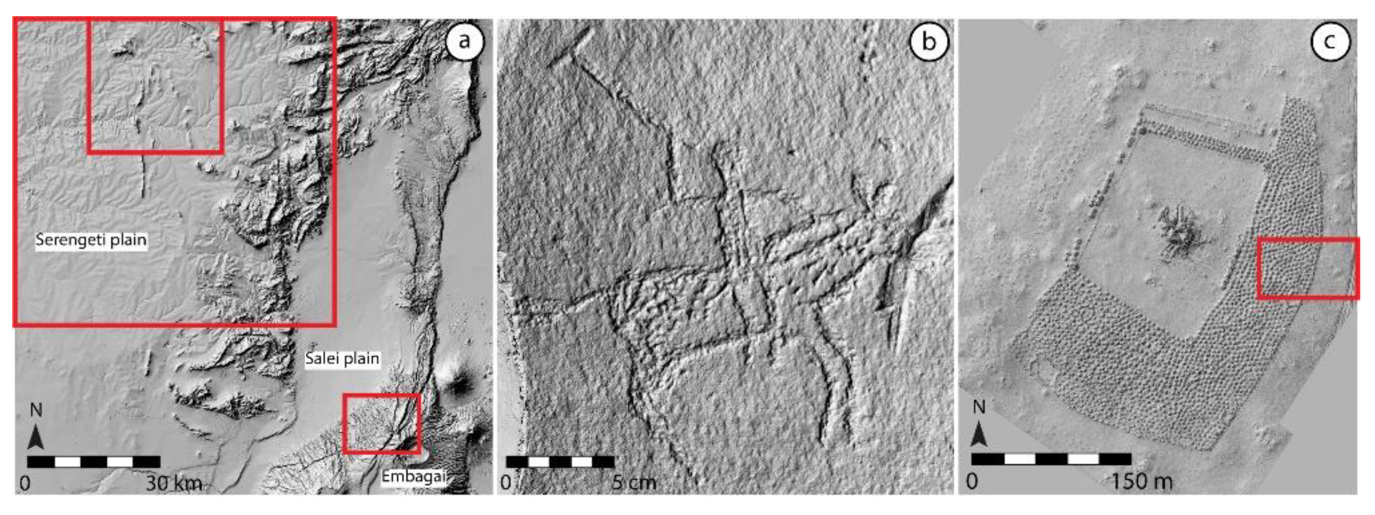
2.1. Corpus
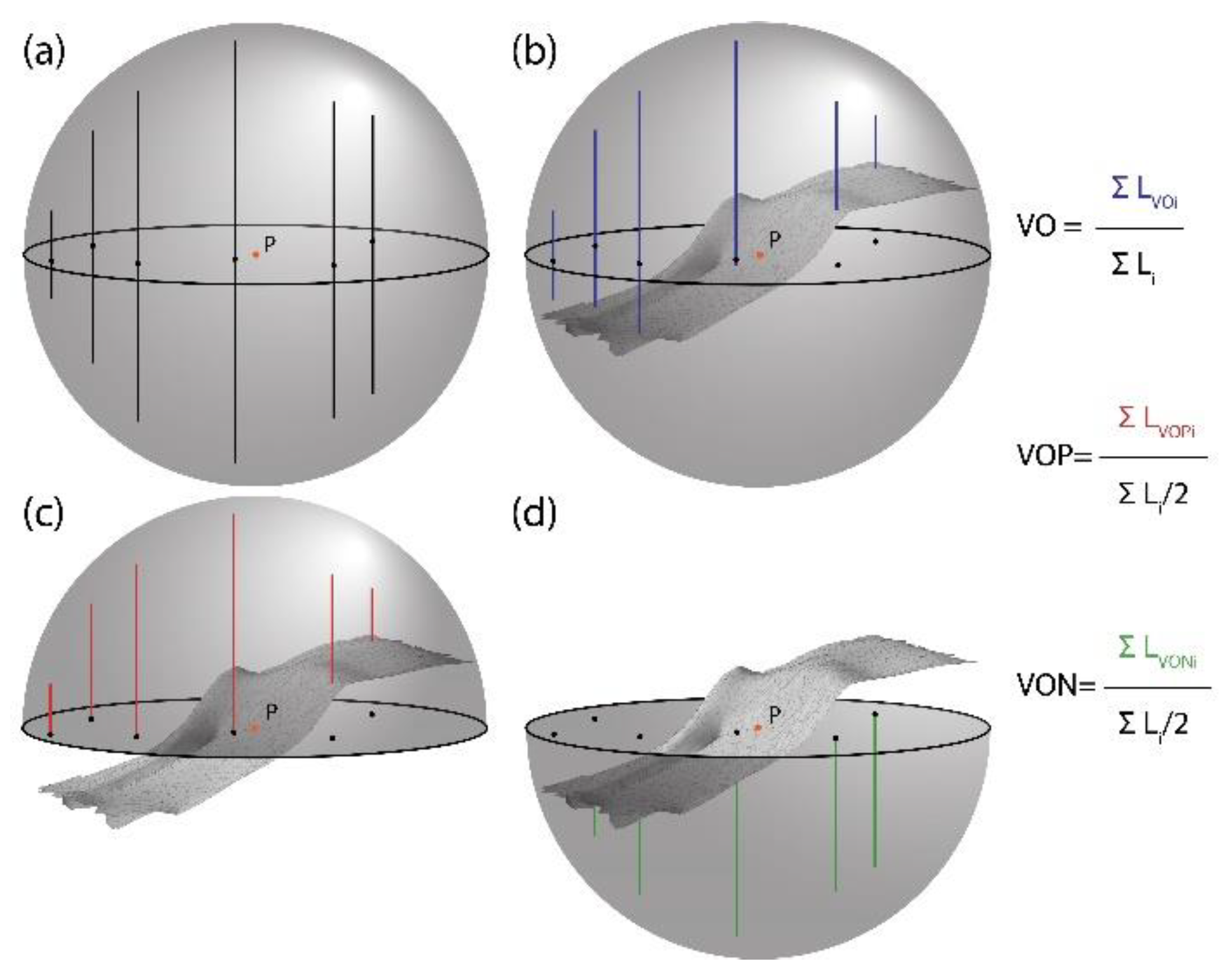
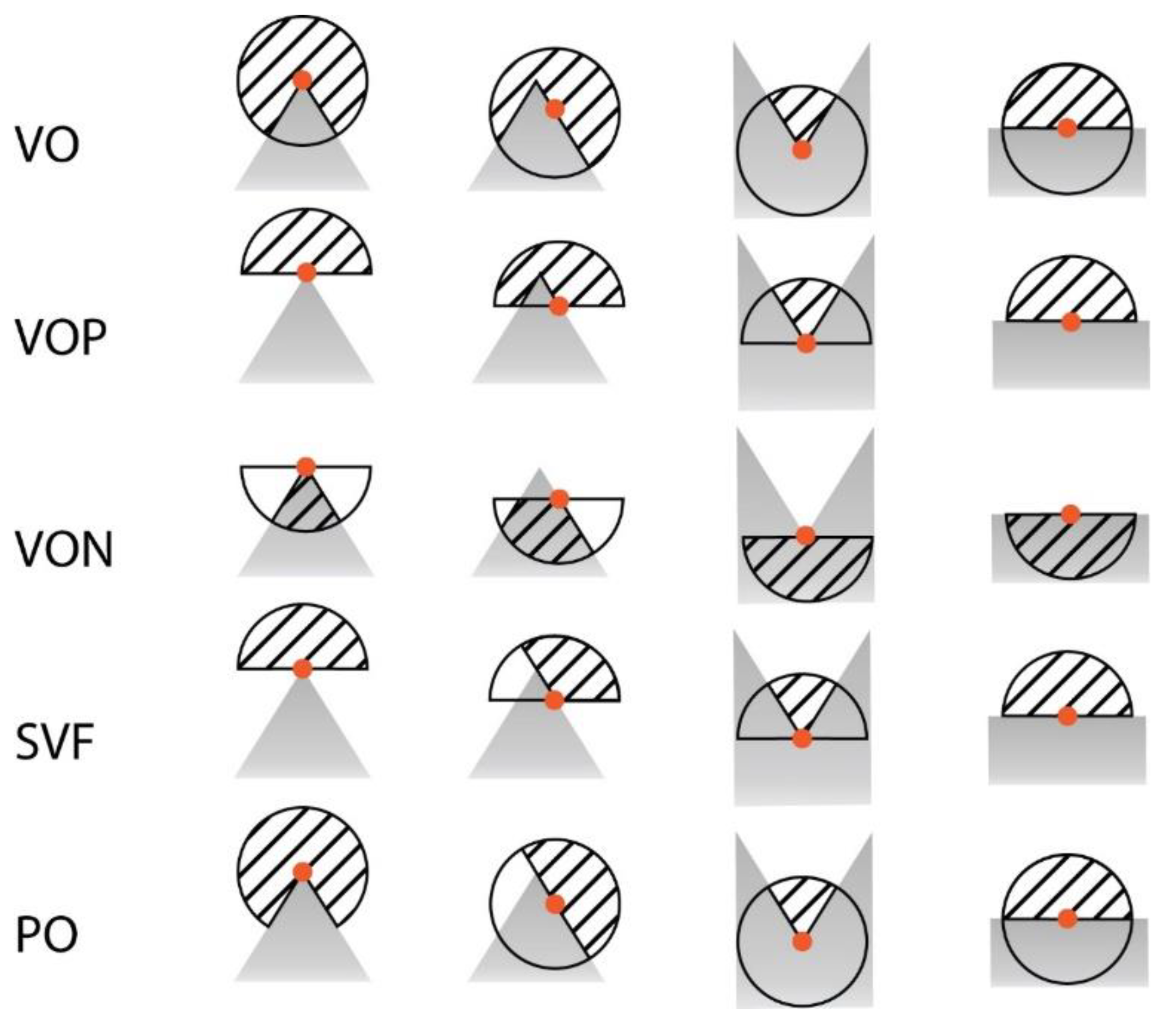
2.2. Volumetric Approach
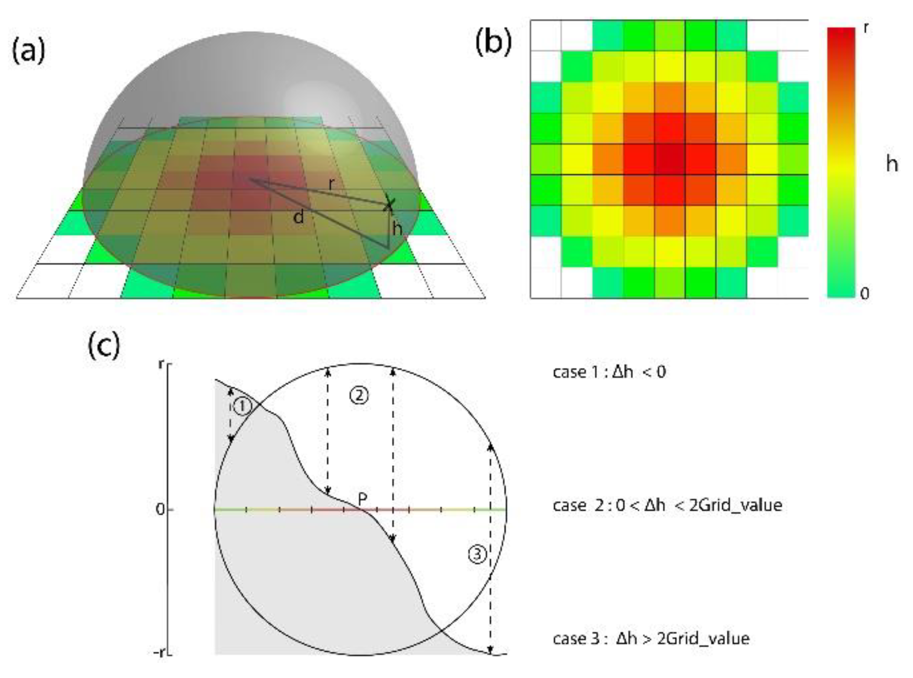
2.3. Algorithm
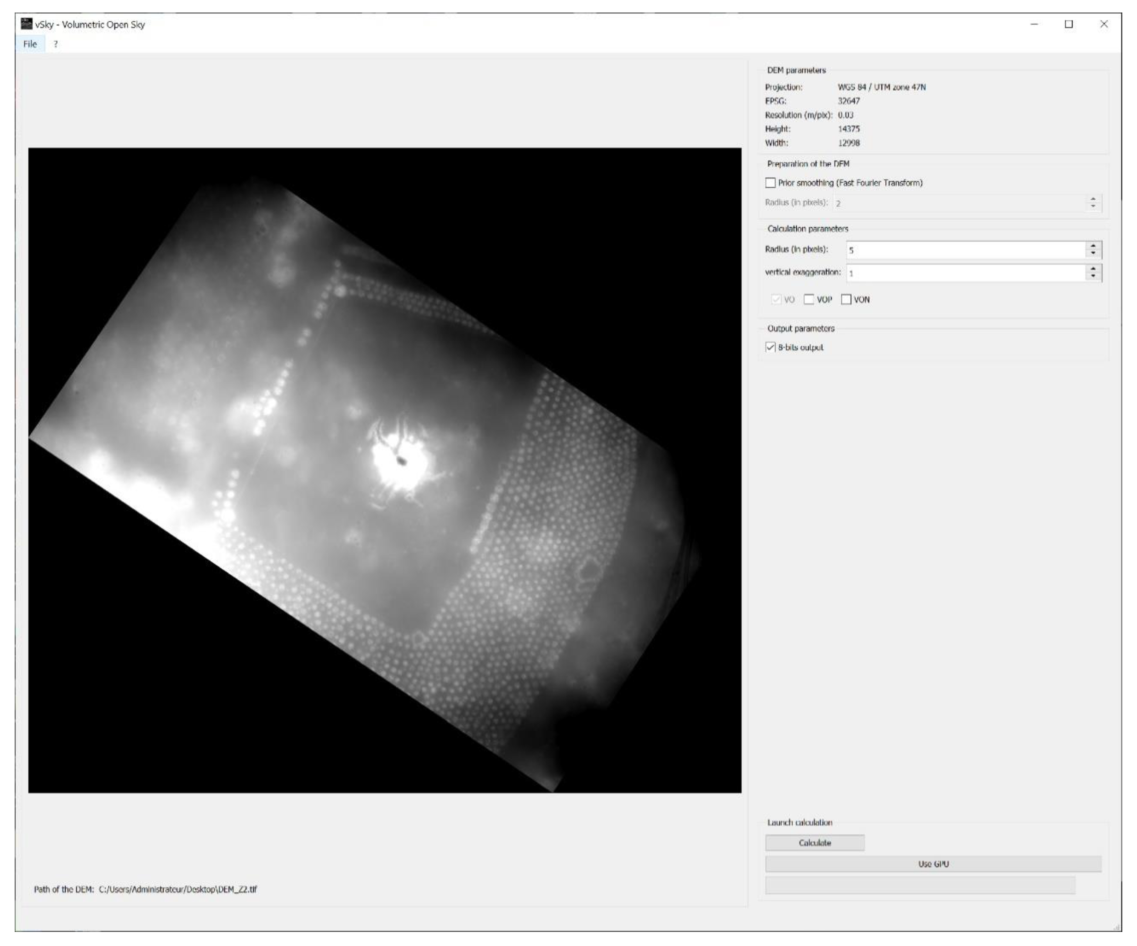
2.4. Implementation
3. Experiments
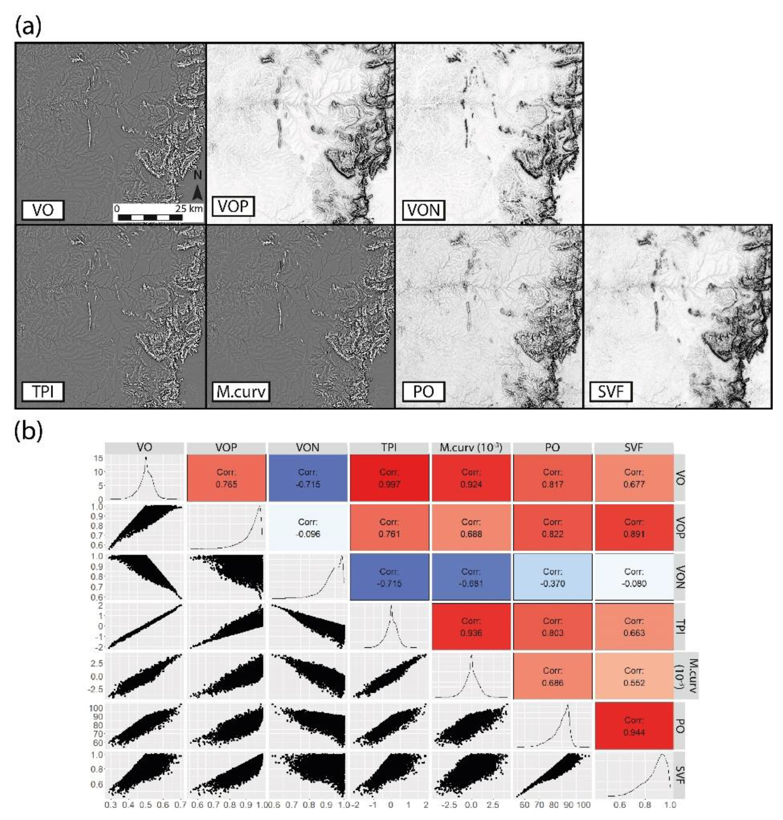
3.1. Algorithm Comparison
3.2. Parameter Influence
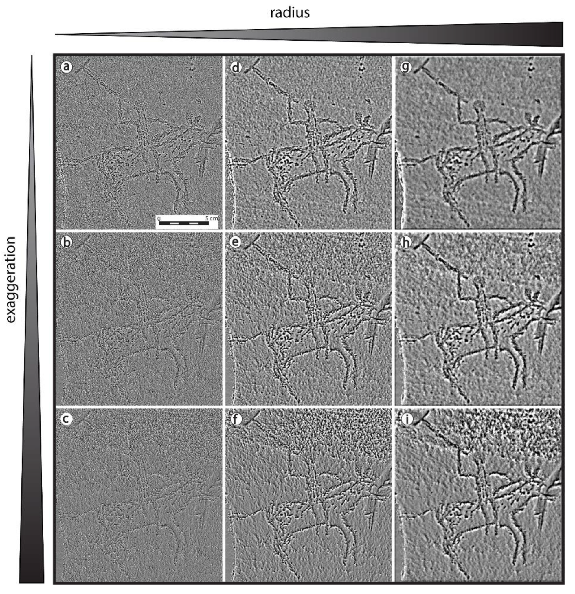
3.2.1. Vertical Exaggeration and Sphere Radius
3.2.2. VO as Feature Input for Automatic Recognition
4. Conclusions
Supplementary Materials
Author Contributions
Funding
Data Availability Statement
Acknowledgments
Conflicts of Interest
References
- Wood, J. The Geomorphological Characterisation of Digital Elevation Models; University of Leicester: Leicester, UK, 1996. [Google Scholar]
- Challis, K. Airborne laser altimetry in alluviated landscapes. Archaeol. Prospect. 2006, 13, 103–127. [Google Scholar] [CrossRef]
- Smith, M.; Goodchild, M.F.; Longley, P.A. Geospatial Analysis: A Comprehensive Guide to Principles, Techniques and Software Tools; Matador: Leicester, UK, 2009. [Google Scholar]
- Longley, P. (Ed.) Geographic Information Systems & Science, 3rd ed.; Fully Updated; Wiley: Hoboken, NJ, USA, 2011. [Google Scholar]
- Minár, J.; Evans, I.S.; Jenčo, M. A comprehensive system of definitions of land surface (topographic) curvatures, with implications for their application in geoscience modelling and prediction. Earth-Sci. Rev. 2020, 211, 103414. [Google Scholar] [CrossRef]
- Hesse, R. LiDAR-derived Local Relief Models—A new tool for archaeological prospection. Archaeol. Prospect. 2010, 17, 67–72. [Google Scholar] [CrossRef]
- Reitberger, J.; Krzystek, P.; Stilla, U. Analysis of full waveform LIDAR data for the classification of deciduous and coniferous trees. Int. J. Remote Sens. 2008, 29, 1407–1431. [Google Scholar] [CrossRef]
- Zakšek, K.; Oštir, K.; Kokalj, Ž. Sky-View Factor as a Relief Visualization Technique. Remote Sens. 2011, 3, 398–415. [Google Scholar] [CrossRef] [Green Version]
- Yokoyama, R.; Shirasawa, M.; Pike, R.J. Visualizing Topography by Openness: A New Application of Image Processing to Digital Elevation Models. Photogramm. Eng. Remote Sens. 2002, 68, 257–265. [Google Scholar]
- Doneus, M. Openness as Visualization Technique for Interpretative Mapping of Airborne Lidar Derived Digital Terrain Models. Remote Sens. 2013, 5, 6427–6442. [Google Scholar] [CrossRef] [Green Version]
- Horn, B.K.P. Hill shading and the reflectance map. Proc. IEEE 1981, 69, 14–47. [Google Scholar] [CrossRef] [Green Version]
- Hobbs, K.F. An investigation of RGB multi-band shading for relief visualisation. Int. J. Appl. Earth Obs. Geoinf. 1999, 1, 181–186. [Google Scholar] [CrossRef]
- Devereux, B.J.; Amable, G.S.; Crow, P. Visualisation of LiDAR terrain models for archaeological feature detection. Antiquity 2008, 82, 470–479. [Google Scholar] [CrossRef]
- Kennelly, P.J.; Stewart, A.J. General sky models for illuminating terrains. Int. J. Geogr. Inf. Sci. 2014, 28, 383–406. [Google Scholar] [CrossRef]
- Jasiewicz, J.; Stepinski, T.F. Geomorphons—A pattern recognition approach to classification and mapping of landforms. Geomorphology 2013, 182, 147–156. [Google Scholar] [CrossRef]
- Hu, G.; Dai, W.; Li, S.; Xiong, L.; Tang, G.; Strobl, J. Quantification of terrain plan concavity and convexity using aspect vectors from digital elevation models. Geomorphology 2021, 375, 107553. [Google Scholar] [CrossRef]
- Kennelly, P.J. Terrain maps displaying hill-shading with curvature. Geomorphology 2008, 102, 567–577. [Google Scholar] [CrossRef]
- Weiss, A.D. Topographic Position and Landforms Analysis; The Nature Conservancy: San Diego, CA, USA, 2001. [Google Scholar]
- Grosse-Brauckmann, K. Triply periodic minimal and constant mean curvature surfaces. Interface Focus 2012, 2, 582–588. [Google Scholar] [CrossRef] [PubMed]
- Langer, M.S.; Zucker, S.W. Shape-from-shading on a cloudy day. J. Opt. Soc. Am. A 1994, 11, 467. [Google Scholar] [CrossRef]
- Phong, B.T. Illumination for computer generated pictures. Commun. ACM 1975, 18, 311–317. [Google Scholar] [CrossRef] [Green Version]
- Mittring, M. Finding Next Gen: CryEngine 2. ACM SIGGRAPH 2007 Courses—SIGGRAPH 07 [Internet]; ACM Press: San Diego, CA, USA, 2007; [cited 29 March 2021]; p. 97. Available online: http://dl.acm.org/citation.cfm?doid=1281500.1281671 (accessed on October 2020).
- Loos, B.J.; Sloan, P.-P. Volumetric Obscurance. Proc ACM SIGGRAPH Symp Interact 3D Graph Games—I3D 10 [Internet]; ACM Press: Washington, DC, USA, 2010; [cited 29 March 2021]; p. 151. Available online: http://dl.acm.org/citation.cfm?doid=1730804.1730829 (accessed on October 2020).
- McGuire, M.; Osman, B.; Bukowski, M.; Hennessy, P. The Alchemy Screen-Space Ambient Obscurance Algorithm. Proc ACM SIGGRAPH Symp High Perform Graph—HPG 11 [Internet]; ACM Press: Vancouver, BC, Canada, 2011; [cited 29 March 2021]; p. 25. Available online: http://dl.acm.org/citation.cfm?doid=2018323.2018327 (accessed on October 2020).
- Holden, D.; Saito, J.; Komura, T. Neural Network Ambient Occlusion. SIGGRAPH ASIA 2016 Tech Briefs [Internet]; ACM: Macau, 2016; [cited 29 March 2021]; pp. 1–4. Available online: https://dl.acm.org/doi/10.1145/3005358.3005387 (accessed on October 2020).
- Bokšanský, J.; Pospíšil, A.; Bittner, J. VAO++: Practical Volumetric Ambient Occlusion for Games. In Eurographics Symposium on Rendering: Experimental Ideas & Implementations; The Eurographics Association: Dublin, Ireland, 2017; pp. 31–39. [Google Scholar]
- Hay, R.L. Geology of the Olduvai Gorge: A Study of Sedimentation in a Semiarid Basin; University of California Press: Berkeley, CA, USA, 1976. [Google Scholar]
- Hay, R.L.; Kyser, T.K. Chemical sedimentology and paleoenvironmental history of Lake Olduvai, a Pliocene lake in northern Tanzania. GSA Bull. 2001, 113, 1505–1521. [Google Scholar] [CrossRef]
- Dawson, J.B. The Gregory Rift Valley and Neogene-Recent-Volcanoes of Northern Tanzania; Geological Society of London: London, UK, 2008. [Google Scholar]
- Pyatkin, B.N.; Martinov, A.I. Shalabolinskie Petroglify; Izd-vo Krasnoyarskogo Universiteta: Krasnoyarsk, Russia, 1985. [Google Scholar]
- Pyatkin, B.N. The Shalabolino petroglyphs on the river Tuba (middle Yenisei). Int. Newsl. Rock Art 1998, 20, 26–30. [Google Scholar]
- Delvet, E. Recent Rock Art Studies in Northern Eurasia, 2005–2009; Oxbow: Oxford, UK; David Brown Book Company [Distributor]: Oakville, CT, USA, 2012; pp. 124–148. [Google Scholar]
- Zotkina, L.V. On the Methodology of Studying Palimpsests in Rock Art: The Case of the Shalabolino Rock Art Site, Krasnoyarsk Territory. Archaeol. Ethnol. Anthropol. Eurasia 2019, 47, 93–102. [Google Scholar] [CrossRef]
- Zotkina, L.V.; Kovalev, V.S. Lithic or metal tools: Techno-traceological and 3D analysis of rock art. Digit. Appl. Archaeol. Cult. Herit. 2019, 13, e00099. [Google Scholar] [CrossRef]
- Kokalj, Ž.; Somrak, M. Why Not a Single Image? Combining Visualizations to Facilitate Fieldwork and On-Screen Mapping. Remote Sens. 2019, 11, 747. [Google Scholar] [CrossRef] [Green Version]
- Gallwey, J.; Eyre, M.; Tonkins, M.; Coggan, J. Bringing Lunar LiDAR Back Down to Earth: Mapping Our Industrial Heritage through Deep Transfer Learning. Remote Sens. 2019, 11, 1994. [Google Scholar] [CrossRef] [Green Version]
- Liu, Q.; Cheng, W.; Yan, G.; Zhao, Y.; Liu, J. A Machine Learning Approach to Crater Classification from Topographic Data. Remote Sens. 2019, 11, 2594. [Google Scholar] [CrossRef] [Green Version]
- Monna, F.; Magail, J.; Rolland, T.; Navarro, N.; Wilczek, J.; Gantulga, J.-O.; Esin, Y.; Granjon, L.; Allard, A.-C.; Chateau-Smith, C. Machine learning for rapid mapping of archaeological structures made of dry stones—Example of burial monuments from the Khirgisuur culture, Mongolia–. J. Cult. Herit. 2020, 43, 118–128. [Google Scholar] [CrossRef]
- Soroush, M.; Mehrtash, A.; Khazraee, E.; Ur, J.A. Deep Learning in Archaeological Remote Sensing: Automated Qanat Detection in the Kurdistan Region of Iraq. Remote Sens. 2020, 12, 500. [Google Scholar] [CrossRef] [Green Version]
- Zakariya Jasim, O. Using of machines learning in extraction of urban roads from DEM of LIDAR data: Case study at Baghdad expressways, Iraq. Period. Eng. Nat. Sci. PEN 2019, 7, 1710. [Google Scholar] [CrossRef]
- Maxwell, A.E.; Pourmohammadi, P.; Poyner, J.D. Mapping the Topographic Features of Mining-Related Valley Fills Using Mask R-CNN Deep Learning and Digital Elevation Data. Remote Sens. 2020, 12, 547. [Google Scholar] [CrossRef] [Green Version]
- Zhao, Z.-Q.; Zheng, P.; Xu, S.; Wu, X. Object Detection with Deep Learning: A Review. arXiv 2019, arXiv:180705511. Available online: http://arxiv.org/abs/1807.05511 (accessed on October 2020).


Publisher’s Note: MDPI stays neutral with regard to jurisdictional claims in published maps and institutional affiliations. |
© 2022 by the authors. Licensee MDPI, Basel, Switzerland. This article is an open access article distributed under the terms and conditions of the Creative Commons Attribution (CC BY) license (https://creativecommons.org/licenses/by/4.0/).
Share and Cite
Rolland, T.; Monna, F.; Buoncristiani, J.F.; Magail, J.; Esin, Y.; Bohard, B.; Chateau-Smith, C. Volumetric Obscurance as a New Tool to Better Visualize Relief from Digital Elevation Models. Remote Sens. 2022, 14, 941. https://doi.org/10.3390/rs14040941
Rolland T, Monna F, Buoncristiani JF, Magail J, Esin Y, Bohard B, Chateau-Smith C. Volumetric Obscurance as a New Tool to Better Visualize Relief from Digital Elevation Models. Remote Sensing. 2022; 14(4):941. https://doi.org/10.3390/rs14040941
Chicago/Turabian StyleRolland, Tanguy, Fabrice Monna, Jean François Buoncristiani, Jérôme Magail, Yury Esin, Benjamin Bohard, and Carmela Chateau-Smith. 2022. "Volumetric Obscurance as a New Tool to Better Visualize Relief from Digital Elevation Models" Remote Sensing 14, no. 4: 941. https://doi.org/10.3390/rs14040941
APA StyleRolland, T., Monna, F., Buoncristiani, J. F., Magail, J., Esin, Y., Bohard, B., & Chateau-Smith, C. (2022). Volumetric Obscurance as a New Tool to Better Visualize Relief from Digital Elevation Models. Remote Sensing, 14(4), 941. https://doi.org/10.3390/rs14040941