Article

Glacier Monitoring Based on Multi-Spectral and Multi-Temporal Satellite Data: A Case Study for Classification with Respect to Different Snow and Ice Types

1
Institute of Photogrammetry and Remote Sensing, Karlsruhe Institute of Technology (KIT), Englerstr. 7, D-76131 Karlsruhe, Germany
2
Department of Geophysics, University of Concepción, Concepción 4030000, Chile
3
Department for Geodetic Sciences and Geomatics, University of Concepción, Los Ángeles 4451032, Chile
*
Author to whom correspondence should be addressed.
Remote Sens. 2022, 14(4), 845; https://doi.org/10.3390/rs14040845
Submission received: 3 December 2021 / Revised: 1 February 2022 / Accepted: 4 February 2022 / Published: 11 February 2022

Abstract

:
Remote sensing techniques are frequently applied for the surveying of remote areas, where the use of conventional surveying techniques remains difficult and impracticable. In this paper, we focus on one of the remote glacier areas, namely the Tyndall Glacier area in the Southern Patagonian Icefield in Chile. Based on optical remote sensing data in the form of multi-spectral Sentinel-2 imagery, we analyze the extent of different snow and ice classes on the surface of the glacier by means of pixel-wise classification. Our study comprises three main steps: (1) Labeled Sentinel-2 compliant data are obtained from theoretical spectral reflectance curves, as there are no training data available for the investigated area; (2) Four different classification approaches are used and compared in their ability to identify the defined five snow and ice types, thereof two unsupervised approaches (k-means clustering and rule-based classification via snow and ice indices) and two supervised approaches (Linear Discriminant Analysis and Random Forest classifier); (3) We first focus on the pixel-wise classification of Sentinel-2 imagery, and we then use the best-performing approach for a multi-temporal analysis of the Tyndall Glacier area. While the achieved classification results reveal that all of the used classification approaches are suitable for detecting different snow and ice classes on the glacier surface, the multi-temporal analysis clearly reveals the seasonal development of the glacier. The change of snow and ice types on the glacier surface is evident, especially between the end of ablation season (April) and the end of accumulation season (September) in Southern Chile.

Graphical Abstract

1. Introduction

Remote sensing surveying techniques are of great advantage for various applications and hence are widely used. On the one hand, they allow for an investigation of large areas in a short time and with less effort than conventional terrestrial surveying methods. On the other hand, as the available set of remote sensing sensors in space is growing, so is the field of possible applications. Among the latter, a particular focus is given to land cover classification, which can be achieved through the evaluation of many different surface properties. In this paper, we study one very remote area, where it would cost an inefficiently high effort to survey with terrestrial approaches. The Campo de Hielo Patagonico Sur (CHPS; also called Southern Patagonian Ice Field) is an icefield in Southern Patagonia between Chile and Argentina. It is the world’s second-largest contiguous extrapolar icefield and the second-largest icefield in the Southern hemisphere after Antarctica [1]. Research in this remote area is still difficult in general as the area is hardly accessible for terrestrial on-site measurements. Consequently, remote sensing was used in the past years to provide access to investigate the area [2].
Due to its large extent, the surveying of ice masses in the CHPS has been of great importance to understand its development over the past and especially recent years to understand the impact of climate change [3,
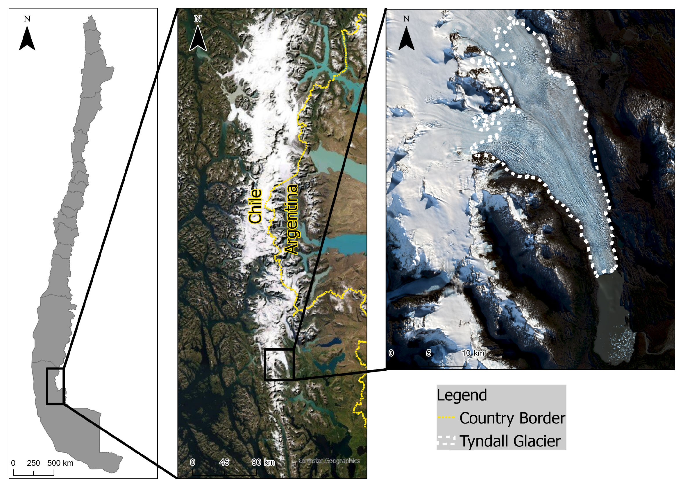
4]. The CHPS is the largest freshwater reservoir in South America [1], providing fresh water to a large part of the dry Patagonian Argentina. The ice mass fed 154 major outlet glaciers until 2011 [5]. Some studies were already carried out on the development of the glacier extent and mass balance through a combination of digital elevation models and optical data [1,6]. However, apart from the knowledge of the glacier extent, the understanding of the land cover types (i.e., the snow and ice types) of the glaciers is of significance, as the variability of seasonal snow cover is an important parameter in the climate system. The type of snow and ice cover of a certain region gives information not only about energy and moisture budgets within the glacier but also is an indicator for surface temperature and precipitation changes [7].

1.1. Contribution

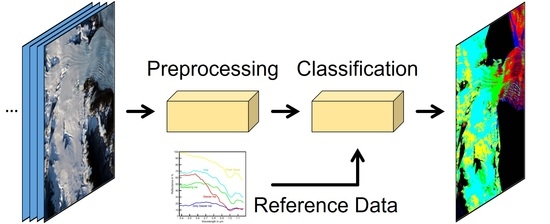
In the scope of our study, the land cover composition on the glacier surface is defined through classification of the snow and ice types on the surface of the glaciers. To investigate the change in glacier extent and surface composition, an evaluation of a time series of specific years is conducted.
This paper extends our previous work [8], where we rely on a pixel-wise classification of Sentinel-2 data with respect to different snow and ice classes. The straightforward approach for this is given by a supervised classification [
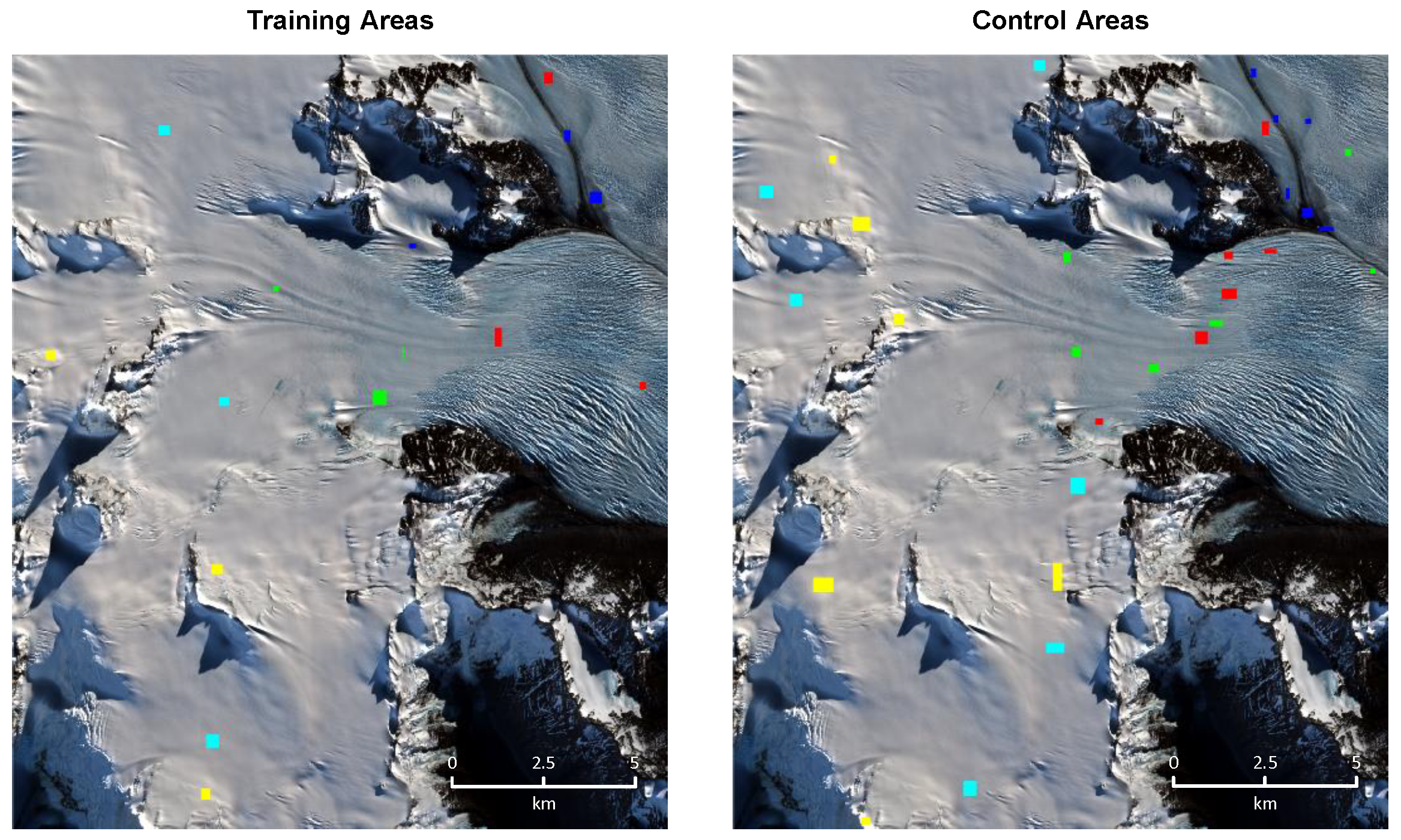
9]. However, no reference data (i.e., training examples) are available for the different snow and ice cover types in the investigated area. Consequently, suitable reference data need to be obtained, for which we rely on theoretical knowledge [10] to simulate labeled Sentinel-2 compliant data from densely sampled spectral reflectance curves representing different snow and ice cover types [11,12,
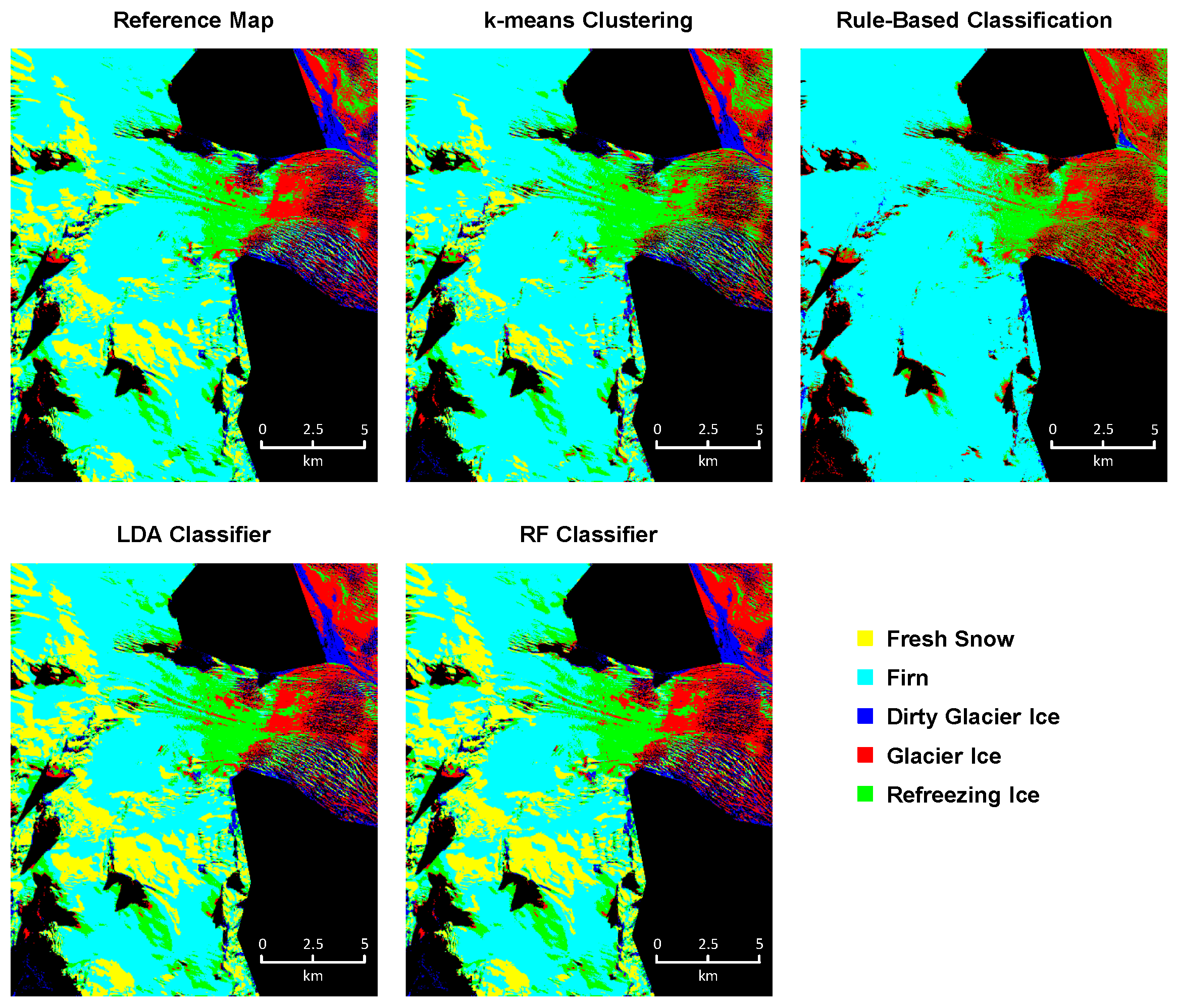
13]. On this basis, we apply four different classification approaches, thereof two unsupervised approaches (k-means clustering [14] and rule-based classification via snow and ice indices [15,16]) and two supervised approaches (Linear Discriminant Analysis [17] and Random Forest classifier [18]). In this paper, our contributions are twofold: (1) We evaluate the given methodology in detail and thereby also deeper analyze the quality of the given reference data; (2) We conduct a multi-temporal analysis to assess changes in glacier extent and surface composition.
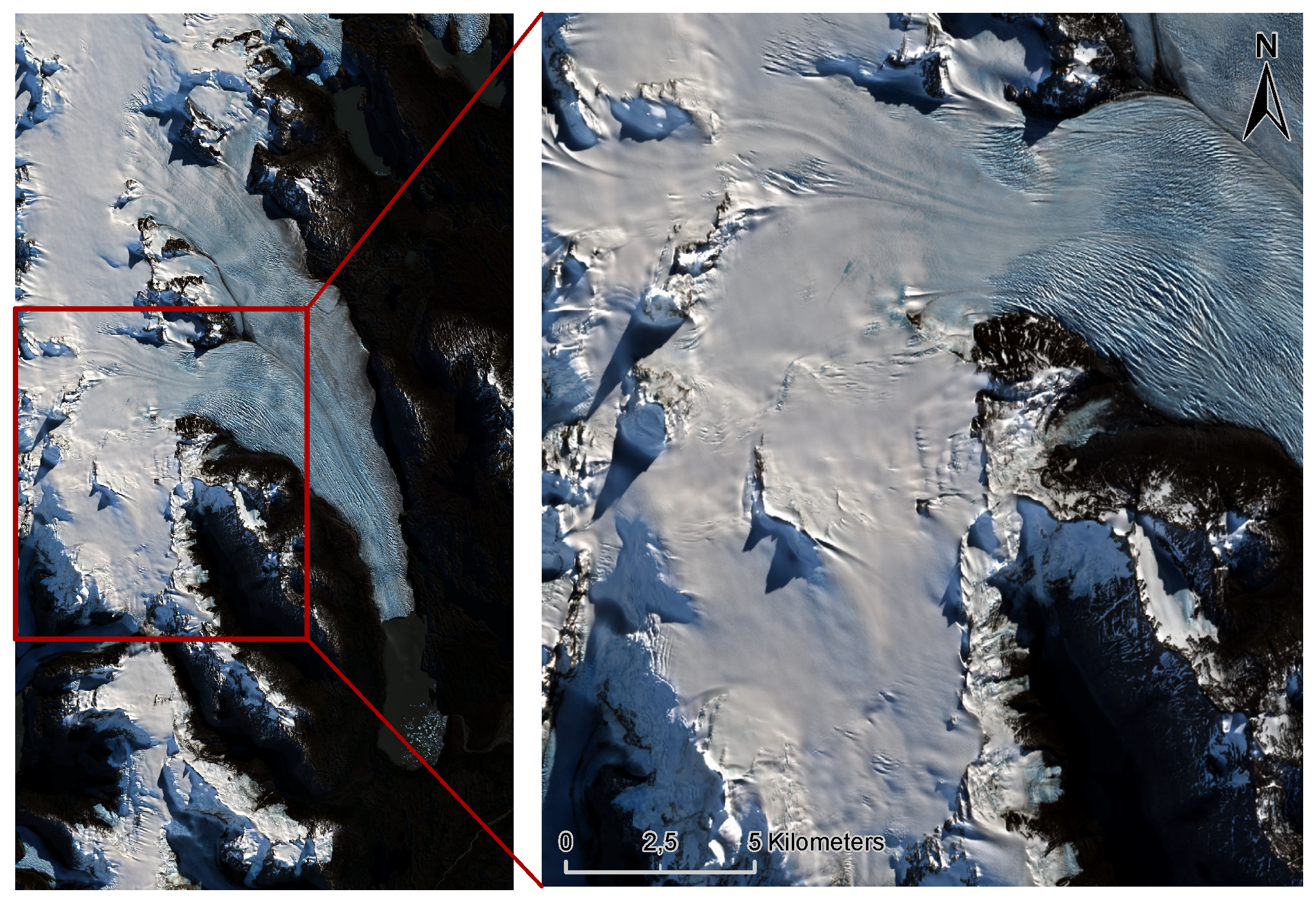
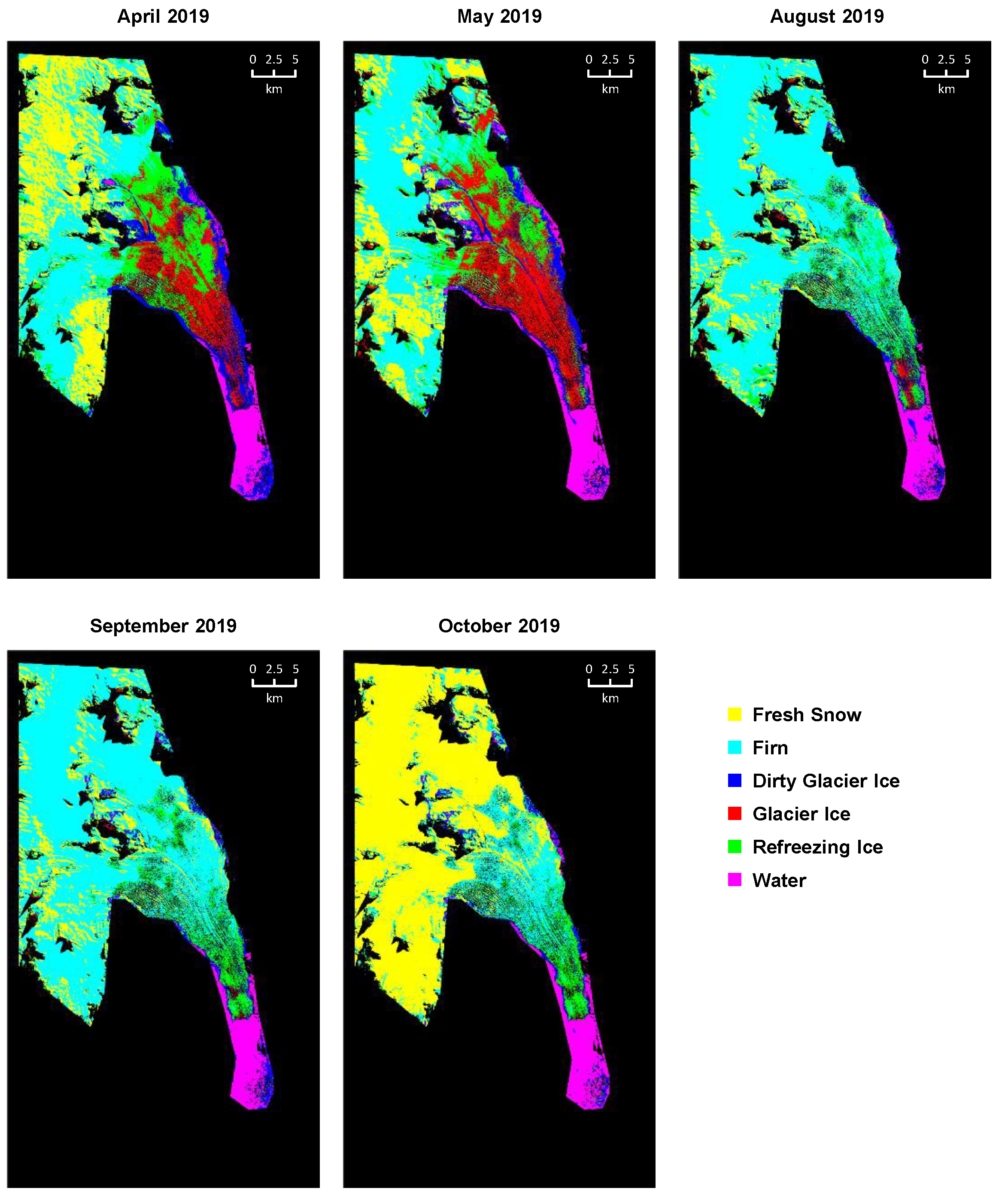
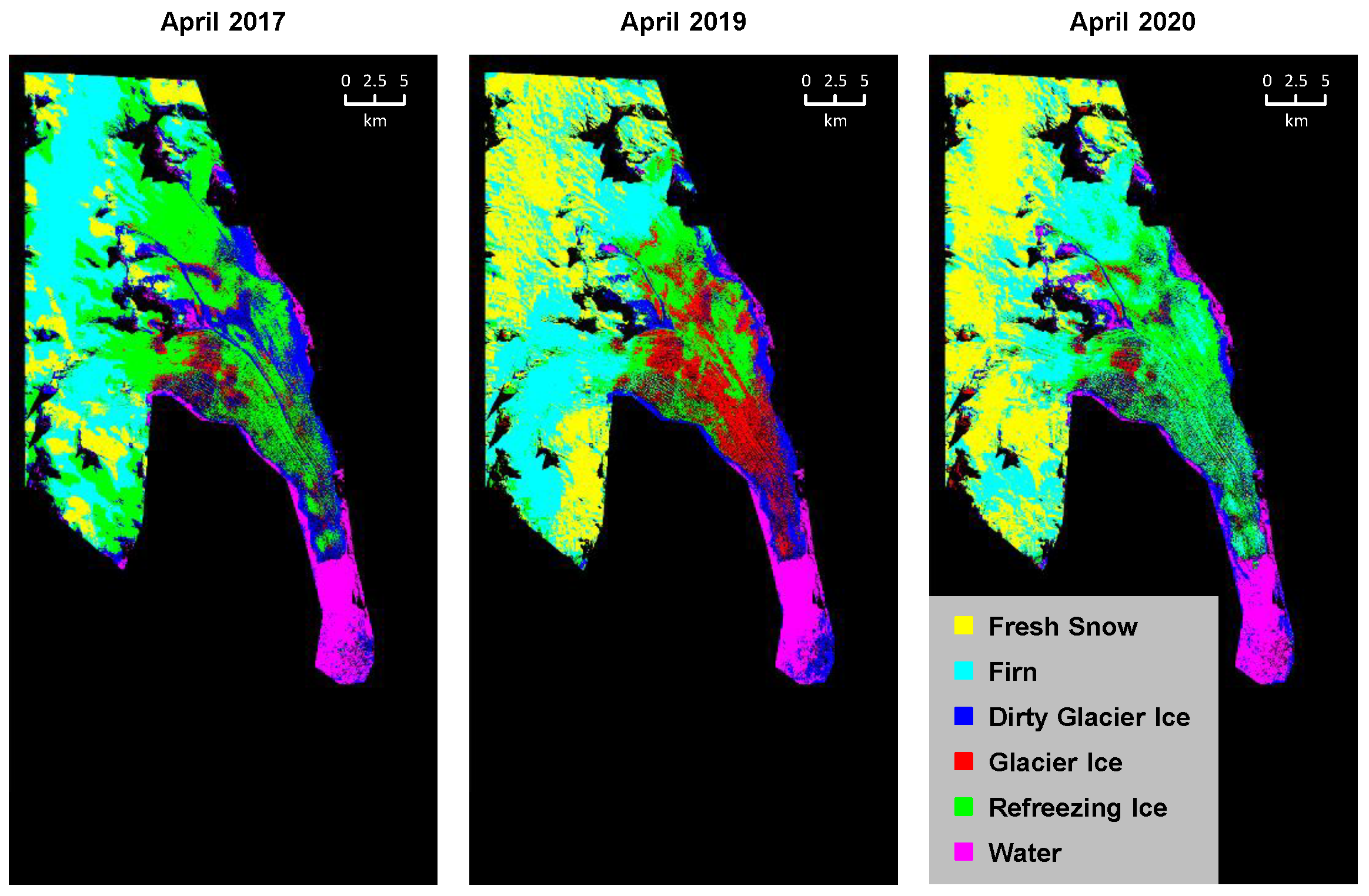
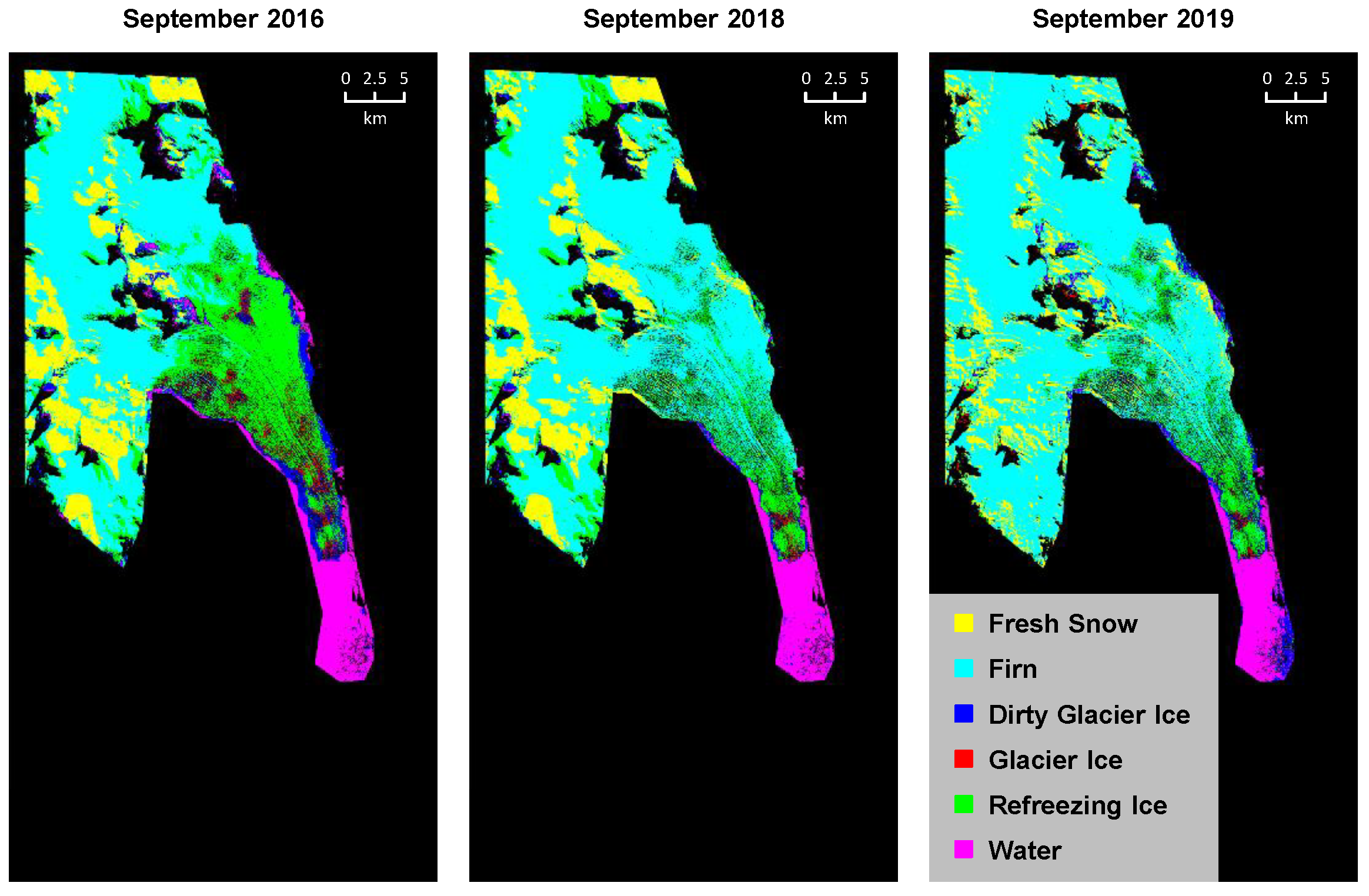
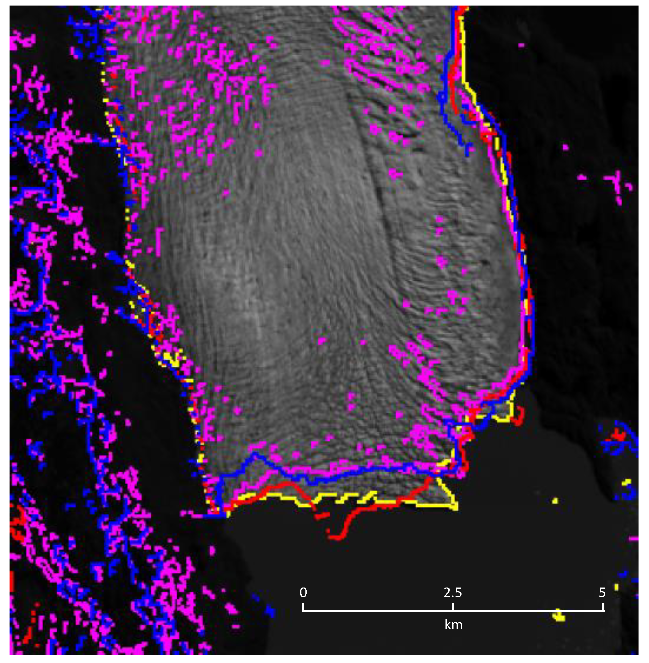
Accordingly, we first focus on the pixel-wise classification of Sentinel-2 imagery available for the Tyndall Glacier area, and we then use the best-performing approach for a multi-temporal analysis. Here, the year 2019 is examined more closely as a representative to demonstrate the findings of the change in glacier surface composition within one year. The dates of the end of ablation and end of accumulation time are investigated subsequently. These dates reveal significant information about the glacier state over the explored timeline of the years 2016 to 2020. The plausibility of the findings is independently evaluated by comparison with temperature and precipitation data. These data mainly influence the glacier’s snow and ice state. Several metrics are applied to demonstrate the classification findings in an intuitive way: Area statistics for each snow and ice class are calculated. Finally, the change in glacier snout extent is described.

1.2. Paper Outline

After briefly summarizing related work (Section 1.3), we present the used materials and methods (Section 2). We first describe the study area (Section 2.1) and the data used for this case study (Section 2.2). Subsequently, we focus on the applied methodology (Section 2.3) and summarize the methodology to obtain labeled reference data (Section 2.3.1) as well as all the algorithms applied for data preprocessing (Section 2.3.2). Furthermore, the involved classification approaches (Section 2.3.3) and the methods applied in the scope of the multi-temporal analysis (Section 2.3.4) are explained. We demonstrate the performance of the proposed methodology by presenting a selection of achieved experimental results (Section 3), and we discuss the achieved results in detail (Section 4). Finally, we draw a conclusion (Section 5) of the findings of the study and we provide an outlook on how to further optimize the results of classification with respect to snow and ice types on a glacier.

1.3. Background

Glaciers play an important role in their influence on climate. According to the Global Climate Observing System (GCOS), glaciers belong to the Essential Climate Variables (ECVs) [19], as glacier changes are key indicators of climate change [20]. Their melting will significantly impact the sea-level rise over the next 100 years [21].
In the context of glacier monitoring, the multi-temporal analysis of a glacier concerning different snow and ice types is relevant to detect changes in the glacier’s surface composition. The glacier influences its environment in different ways through melting or refreezing on the glacier [22,23]. Its surface composition gives information about energy and moisture budgets within the glacier and is an indicator for surface temperature and precipitation changes [7]. This influence can be estimated from the extent of snow and ice classes on the glacier’s surface, which demonstrates the state of melting or refreezing.
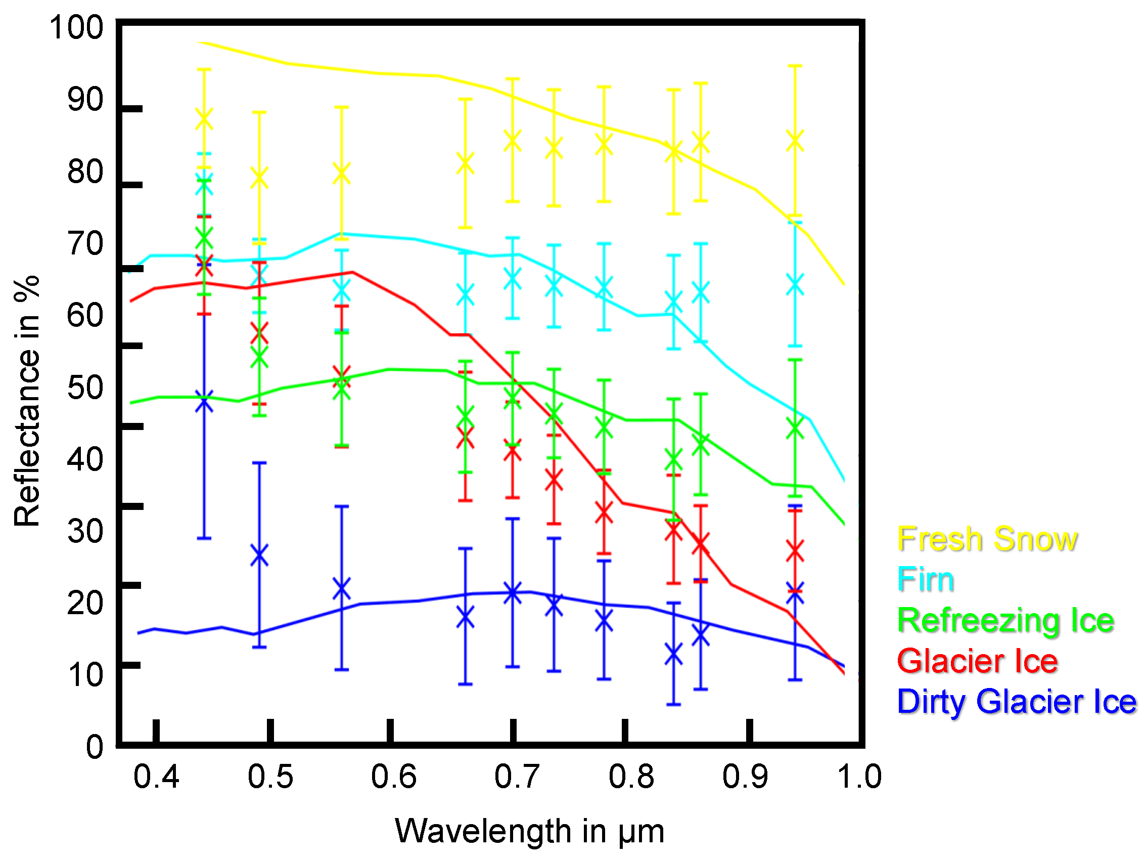
To analyze the extent of different snow and ice classes on the glacier’s surface, corresponding target classes for the classification task need to be defined. There exist different definitions of snow or ice types [24] or glacier zones [25], which have been derived according to several physical properties. Therefore, the task of snow and ice type definition is essential to delimit possibly distinguished classes. The characteristics of the snow and ice types alter the spectral signature of the different snow and ice types in the multi-spectral satellite imagery and can therefore be detected through classification of the optical imagery [8]. The definitions used in our work rely on the classes used in [10,26,27,28] and specified by one spectral signature per class, covering wavelengths between about 0.4 μm and 1.2 μm. However, these classes do not correspond with other snow and ice class definitions like, for example, given in [29,
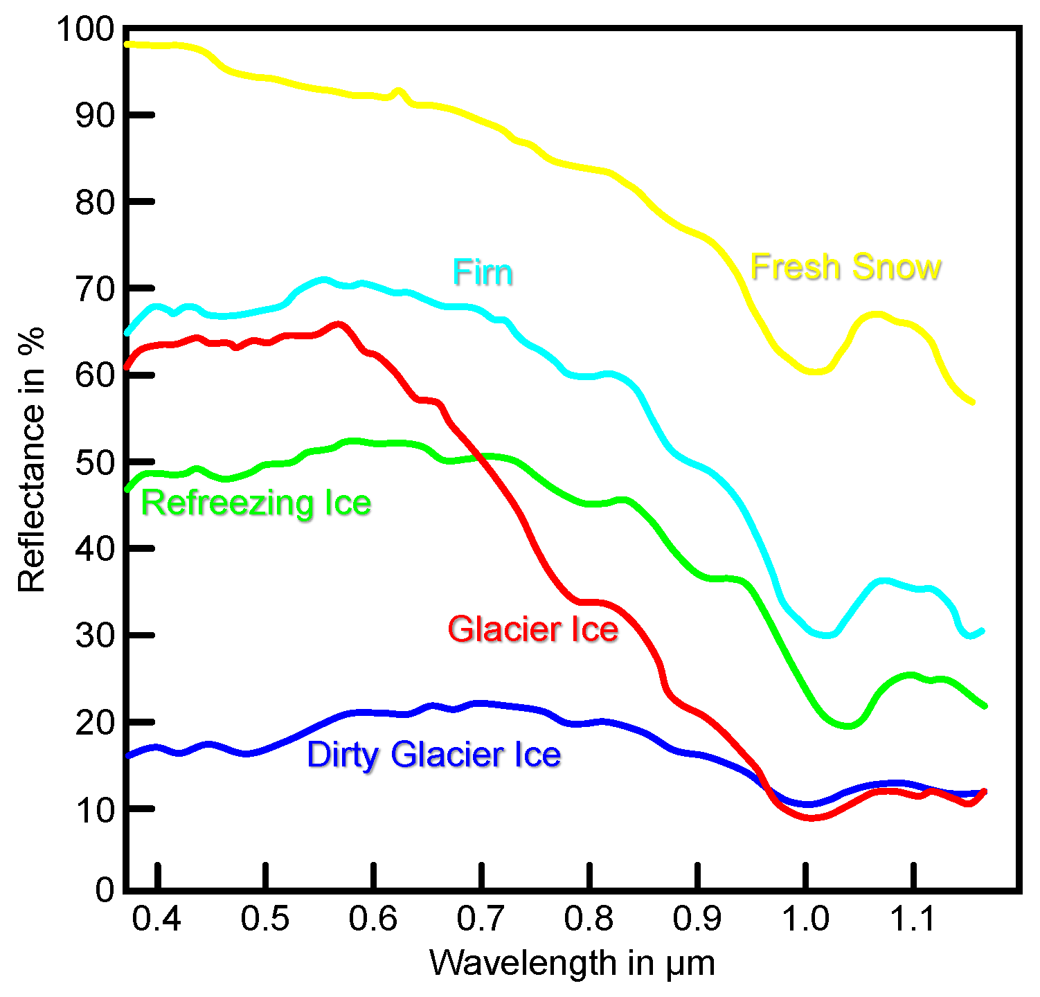
30], since definitions there rely on radar systems and thus different wavelengths, resulting in different characteristics that are revealed by the acquired data. The classes considered in the scope of our work can be briefly described as follows:
  • Glacier Ice: This ice type is formed when fallen snow is compressed and slowly turning into ice. This process occurs, where the accumulation of snow and ice exceeds ablation and where different geological criteria are met. Glacier ice typically exists in the lower parts of a glacier;
  • Refreezing Ice: This ice type occurs when snow falls on already existing ice. The fresh snow is compressed and becomes part of the glacier. Compared to glacier ice, refreezing ice typically exists in the upper parts of a glacier and is newer ice;
  • Dirty Glacier Ice: This ice type contains small impurities within the ice. These impurities are mostly bare soil or rock material debris lying on the glacier or adjacent to the glacier, and even small impurities of soil can cause a different spectral reflectance of the ice;
  • Firn: This snow type is characterized by being melted and refrozen. Therefore, it contains a higher water content than Fresh Snow and more impurities. More specifically, due to changes in incident solar radiation and temperature, fallen snow melts and refreezes in certain intervals. Snow that traversed this process once or several times is commonly defined as Firn [25,26,27,28,29], but sometimes also as AgedSnow [10];
  • Fresh Snow: This snow type represents newly fallen snow that did not go through the process of melting and refreezing. It has lower water content and contains fewer impurities in comparison to Firn.
Note that these classes only describe transient states of the snow and ice, which can quickly transform into other states (and therefore classes), depending on several natural conditions. Some of these classes (FreshSnow, Firn, Refreezing Ice) might therefore quickly lose their distinguishing characteristics that influence the spectral reflectance. However, these classes are of great interest for glacier monitoring, and the motivation for using these classes seems intuitive: The deeper the snow depth, the bigger the delay in time to reach isothermal conditions, which allows the snow cover on the glacier to persist longer [31]. Thus, it prevents more melting and water run-off from the glacier. The separation into the classes of Fresh Snow and Firn allows statements about the snow wetness, one of the main physical properties of snow. Snow wetness accordingly allows statements about the location of zones of accumulation areas on the glacier. Concerning the ice classes, three classes are distinguished. On the one hand, the performed separation allows reasoning about the extent of debris cover on the glacier surface. Debris cover influences the glacier behavior, as surface debris affects the rate of glacier melting [32]. On the other hand, the separation of Refreezing Ice is relevant, as the refreezing of meltwater may prevent immediate run-off of meltwater and therefore also influences glacier ablation in another way than Glacier Ice [33].
Several approaches exist to apply remote sensing techniques for glacier observation. In this context, numerous studies focused on the development of the glacier extent and mass balance of glaciers in general. The extent of glaciers was, for instance, investigated in [34,35,36]. Mass balance can be estimated through optical remote sensing [37] and the combination of digital elevation models and optical remote sensing data, which is quite commonly applied [6,38,39,40]. Some studies were carried out on the mass balance of the here investigated Tyndall Glacier [1,41].
Other studies suggest several different approaches for glacier observation. These can employ different sensors that make use of other segments of the electromagnetic spectrum. Taylor et al. [42] give an overview of several innovations of usable sensors. Besides optical remote sensing, SAR remote sensing can be used for snow and ice cover investigations [43,44,45,46], alike thermal infrared remote sensing [47,48].
Using only optical satellite data, a diversity of techniques may be applied for glacier monitoring. Dietz et al. [10] highlight remote sensing methods considering snow properties in different wavelengths. Rabatel et al. [49] present three different methods for mass balance determination: the ELA (equilibrium-line altitude) approach, the albedo approach and the snow map approach. Few studies focus on the categorization of specific snow and ice classes on the glacier area. The albedo approach and the snow map approach proposed by Rabatel et al. [49] belong to these studies. The albedo approach is based on the principle of the evocation of different spectral responses by distinct snow and ice classes. Therefore, the specific spectral reflectances of the distinct snow and ice classes need to be known. Dietz et al. [10] give an overview of the reflectances of different surface types related to snow cover in a different wavelength. The reflectances of several different glacier states and locations and other large ice accumulations, where the classification into snow and ice classes might be advantageous (e.g., Antarctica), vary a lot [50]. Takeuchi et al. [51] show the specific surface albedo on the Tyndall Glacier, which is also the area of interest in our study, but without an assignment of specific classes to certain albedo values. Baraka et al. [52] propose a deep learning approach to categorize the classes of clean and debris-covered ice. Similar works focused on the mapping of debris-covered glaciers [53,54] or the identification of rock glaciers [55] for Himalayan areas.
Besides supervised approaches, rule-based approaches and unsupervised approaches are already applied for snow cover classification. Wang and Li [56] use the Normalized Difference Snow Index (NDSI) in combination with supervised approaches. Another snow mapping method is based on regional snow maps from daily optical satellite images, where the first step also consists in calculating the NDSI [49]. Combinations of three different snow indices to distinguish four classes allow an even more sophisticated separation [15]. Here, a thresholding is applied to assign each pixel to either class. Gupta et al. [57] use only the NDSI and thresholding. Paul et al. [16] and Zhou et al. [58] use band ratios and thresholding for glacier extent mapping. DeAngelis et al. [2] use an unsupervised (k-means and ISOdata clustering) and supervised (max likelihood) approach for a classification with respect to the classes of Bare Ice, Debris-covered Ice, Slush, Snow-1, Snow-2 and Shadows.
Overall, many studies have been carried out to map glacier extent and obtain mass balance. In contrast, a classification into snow and ice classes was rarely realized. Considering all possibilities optical remote sensing data offer to carry out this study, we decided to use Sentinel-2 data and four different classification approaches, two supervised and two unsupervised ones (according to [8]). These approaches are used as the basis for further investigations and development in our study.
Multi-temporal analyses have been widely used for change detection over several years in all fields based on remote sensing data. In this regard, many studies (see, for example, [59,60]) focus on land cover change detection with Sentinel-2 data. Specialized in the field of study on glacier change detection, Cao et al. [61] conduct a multi-temporal analysis on the changes in glacier volume, and others on the development of the glacier extent over time [62,63]. Asokan et al. [64] give an overview of different change detection techniques in general.
Several studies consider the same area of investigation as in this study [2,65]. The Patagonian Icefield and its glaciers are of major interest as they have been significantly retreating for some years [1] and may contribute significantly to sea-level rise [3,4]. We specifically focus on one glacier in the CHPS, the Tyndall Glacier. It already has been investigated in particular in several studies [6,41].

2. Materials and Methods

In the scope of this paper, we consider a change detection task relying on the classification of Sentinel-2 imagery across multiple acquisition times. More specifically, we address glacier monitoring in terms of analyzing the extent of different snow and ice types on the glacier surface, as the variability of seasonal snow cover on the glacier surface is an important parameter in the climate system. First, we present the study area (Section 2.1) for this case study as well as the input data (Section 2.2) for the classification task. The input data are multi-spectral satellite data in the form of Sentinel-2 imagery on the one hand and theoretical spectral signatures for training and evaluation on the other. Subsequently, we explain the methods applied in the scope of our study (Section 2.3), for which an overview is provided in Figure 1. As no labeled benchmark dataset exists for the considered classification task, we first need to generate reference data matching the given class definitions (Section 2.3.1). Then, we focus on the preprocessing of the multi-spectral data (Section 2.3.2) and the classification with respect to the given different snow and ice types (Section 2.3.3), where the latter is approached with four different classification approaches. Finally, after the classification of data of several time steps, the results are merged to conduct the multi-temporal analysis using different methods (Section 2.3.4).

2.1. Study Area

The Southern Patagonian Icefield (Campo de Hielo Sur; CHPS) in Chile and Argentina stretches from parallels 48°15′S to 51°30′S for approximately 350 km [66] and covers an area of 12,363 km2. The extent of the entire icefield is too large to undertake a study of precise snow/ice type classification. Hence, in this study, only a subset of the Torres del Paine National Park is considered. This subset still represents a great physical, climatic and biological diversity [67]. The national park is a gateway for human interaction with the otherwise untouched wilderness of major parts of the rest of the CHPS. This national park comprises the Grey Glacier, the Tyndall Glacier, and the Dickson Glacier. Representatively for these three glaciers, that are influenced by the same climatic and weather changes, the snow and ice cover development of the Tyndall Glacier is studied, which is one of the largest glaciers in the Southern Patagonian Icefield, with an approximate length of 32 km and an extent of 331 km2 [41]. It is also one of the southernmost glaciers in the CHPS and is retreating in an enlarging terminus lake. Its location is displayed in Figure 2.

2.2. Data

For our study, we use multi-spectral Sentinel-2 data to benefit from the high resolution of 10 m for at least four of its 13 spectral bands. The scenes are available on the satellite mission’s download platform (Copernicus Open Access Hub). A time series of several years should be evaluated to investigate the change of the glacier surface cover over time. At this stage, the available years 2015 to 2020, when Sentinel-2 was operational, are evaluated. As for 2015, the area is cloud-covered for most acquisition dates, this year will not be considered in general. Some considerations already address the best survey timing and frequency: According to the studies of Karpilo et al. [68], glacier monitoring timing depends on the different characteristics, which are to be surveyed. To allow the determination of the glacier’s terminus position (the position of the snout of the glacier), the survey should be carried out in the late summer. This is the end of the ablation season and when the maximum area of snow-free ice is exposed. In the area of the Torres del Paine National Park, this state coincides with the months of February to April. For determining the magnitude of seasonal accumulation/ablation (mass balance), the survey should be carried out at the end of the accumulation season and at the end of the ablation season, respectively. In the area of the Torres del Paine National Park, the state of the end of accumulation season coincides with the months of September/October. Monitoring should occur on an annual basis for the terminus position and naturally biannually for the mass balance. As snow/ice melt occurs mainly in the Chilean summer (December–February) and continues in the months after (March/April), mainly these months should be investigated [68]. We need to adapt the investigated months slightly, as days without cloud cover or at least partial cloud cover are rare for the study area.
Other data necessary for the classification task are the reference data. These are obtained from theoretical knowledge, as no ground truth data or adequately labeled benchmark data are available with respect to the different snow and ice cover types in the investigated area. According to the studies of Dietz et al. [10], the reflectance values obtained in a certain wavelength of the sensor’s spectrum are related to the snow/ice cover type. The corresponding spectral signatures for either class are represented in Figure 3 in Section 2.3.1. These were derived over an area in Northern China, and they reveal that the classes meaningful for the aim of our study can, in principle, be differentiated well.
Besides relying on theoretical knowledge in the form of these spectral signatures for the defined classes, we additionally consider the class Water, as we pursue a classification of the complete scene for the multi-temporal analysis. The class Water is essential, as the glacier snout retreats in a terminus lake, and we clearly need to determine a transition from the snow and ice classes present on the glacier to the non-ice class of the lake. A clear distinguishing by classifying all the classes (including water) allows the inference to the development of the glacier retreat in the multi-temporal analysis. Hence, labeled reference data are also necessary for the class of Water. Therefore, another reflectance curve is used to provide the necessary theoretical data basis for this class.

2.3. Methods

In this section, we first explain how reference data are created for the classification task (Section 2.3.1). Subsequently, we describe the performed data preprocessing (Section 2.3.2) and the applied classification approaches (Section 2.3.3). This part of our methodology is following our previous work [8], yet described in more detail and with additional classifier settings. Finally, we focus on change detection by applying the classification approaches on Sentinel-2 data of the study area across multiple time steps, as this allows for a multi-temporal analysis in terms of change detection with respect to glacier extent and surface composition (Section 2.3.4).

2.3.1. Generation of Reference Data

As in this case, the study area is inaccessible to terrestrial surveys in a reasonable effort, no ground truth data are available. Suitable reference data are therefore obtained from theoretical knowledge according to a methodology described in our previous work [8]. For the predefined target classes, we take into account spectral signatures defined according to [10,26] for the classes of interest for an area in Northern China (Figure 3).
Relying on this theoretical knowledge in the form of a spectral signature per snow/ice cover type as reference, we assume that a transfer to our study area can be made by comparing measured spectral signatures to this reference and accordingly selecting similar samples as training data. However, the measured signatures are acquired with the Sentinel-2 Multi-Spectral Instrument (S2-MSI), thus represented by 13 reflectance values corresponding to the 13 given spectral bands. Consequently, we need to simulate labeled Sentinel-2 compliant data from the reference signatures of the different snow and ice cover types. To do so, we apply an interpolation of the reference signatures to obtain the spectral reflectance curves (SRCs) with values for steps of 1 nm in wavelength. Subsequently, the spectral response functions (SRFs) of the S2-MSI and the derived SRCs are used to calculate the weighted mean of the spectral reflectance values (SRs) per class per band. As a result, we get one Sentinel-2 compliant spectral signature as reference for each of the five classes of interest (i.e., Glacier Ice, Refreezing Ice, Dirty Glacier Ice, Firn and Fresh Snow).
As one Sentinel-2 compliant spectral signature per class does not reflect the whole variance of spectral values within one class, the creation of a bigger dataset is necessary regarding the training of a supervised classification approach. For this purpose, we focus on selecting similar samples from our study area via the Nearest-Neighbor (NN) algorithm.
In the next step, training data (Training Areas = TAs) and test data (Control Areas = CAs) are created to obtain a non-committed result in the evaluation of classification results. To set up the TAs and CAs, independent Regions Of Interest (ROIs) are selected manually on the glacier area, based on the data created through the NN algorithm and according to standard criteria like representativeness and spectral variability. As for the classification of full scenes of the glaciers, the class Water is added, labeled reference data are also necessary for this class and generated accordingly from a given spectral reflectance curve [69].

2.3.2. Preprocessing

Suitable Sentinel-2 imagery of our study area is selected by choosing the least-cloudy scene for each month of the year 2019 and the selected months lying in the ablation or accumulation time of the years 2016 to 2020. No scene is chosen for a month if the cloud cover is >50% in the study area for all scenes of the month. When using Sentinel-2 satellite data, some preprocessing steps are required concerning the data. First, an atmospheric correction via the Sen2Cor software is applied according to [70], which involves the following steps:
  • Look-Up-Table (LUT) preparation;
  • retrieval of Aerosol Optical Thickness (AOT);
  • retrieval of Water Vapour (WV);
  • cirrus removal; and
  • the retrieval of the corresponding surface reflectance.
Next, we apply an image enhancement for each band of the multi-spectral imagery, that is, for each image in the corresponding image stack. For that purpose, values that lie below or above the boundary 1%-percentile are cropped and mapped to the percentile’s value corresponding to the considered band. Then, the resulting values for each band are scaled to a range of 0% to 100%. Finally, a resampling to a resolution of 10 m is applied for those Sentinel-2 bands with lower resolution.
As only the glacier itself is relevant for our study, while the area surrounding the glacier is not of particular interest, a corresponding image mask is created via manual annotation. Furthermore, in some scenes, shadow areas exist on the glacier. These areas are discarded by applying a shadow mask created automatically via transformation to another color representation [71] and subsequent clustering. Since different scenes can have slightly different viewing angles and therefore shadows, such masks are created for two different scenes that show the maximal extent of shadows and are combined subsequently. Hence, all possible shadow extents are excluded by one mask that can be applied to all investigated scenes.

2.3.3. Classification

For a pixel-wise classification of the given Sentinel-2 data with respect to the different snow and ice classes, we test four different classification approaches. On the one hand, we involve two unsupervised approaches represented by a standard k-means clustering and a rule-based classification via snow and ice indices. On the other hand, we involve two supervised approaches represented by Linear Discriminant Analysis (LDA) and Random Forest (RF) classifiers.
For the k-means clustering, the parameter k is selected as a suitable number of centroids [14] derived experimentally for the given classification task. The obtained clusters after the clustering step are assigned to the predefined classes (Section 1.3) based on their Euclidean distance to the respective reference spectra.
For a rule-based classification approach, different spectral indices to separate between different snow cover classes were used [15]. These indices are the Normalized Difference Snow Index (NDSI), the Normalized Difference Glacier Index (NDGI) and the Normalized Difference Snow Ice Index (NDSII):
N D S I = G R E E N S W I R G R E E N + S W I R
N D G I = G R E E N R E D G R E E N + R E D
N D S I I = G R E E N N I R G R E E N + N I R .
After calculating these indices, thresholds are applied to separate the data for the classes [15]. Suitable thresholds are chosen experimentally, since the thresholds vary with different sensors and seasons. To compare the thus achieved results with the other classification approaches, we need to adapt the class definitions used in [15] towards our predefined classes.
For the LDA classifier, we assume that each of the classes is characterized by a mean vector μ i and the same covariance matrix Σ . Gaussian distribution parameters can then be estimated for each class during the training relying on training examples. By maximizing the likelihood, a label can be assigned to each data point to be classified.
The RF classifier [18] relies on the idea of strategically generating an ensemble of decision trees via bootstrap aggregating: A number of weak learners represented by decision trees are trained independently from each other on subsets of the training data, which are randomly drawn with replacement. For a new sample to be classified, each decision tree casts a vote for one of the defined classes, and the majority vote across the individual votes is typically used for a robust class prediction. In contrast to the other classifiers involved in our study, the RF classifier relies on internal hyperparameters. In this study, we particularly pay attention to the hyperparameters represented by the number M of decision trees and the maximum tree depth M a x D of each decision tree, while further hyperparameters (e.g., the minimum allowable number n min of training examples for a tree node to be split or the number n a of active variables to be used for the test in each tree node) are selected as default values according to the most commonly used implementations. The RF’s hyperparameters are optimized with a grid search on a suitable raster of values for the involved free hyperparameters.
Among all classification approaches, the supervised ones are trained on exemplary datasets (see Section 2.3.1), while each classification approach provides a classification map for the considered scene for every selected time step.

2.3.4. Multi-Temporal Analysis

For the multi-temporal analysis, all preprocessing steps as described above are carried out accordingly for all time steps to be investigated. Thus, we get a pixel-wise classification result per time step, and a comparison of these classification maps allows reasoning about changes in glacier extent and surface composition.
Several methods are applied to investigate the change detection, that occurs in the comparison of classification results derived for different time steps. On the one hand, land cover area statistics are calculated for each time step and compared. On the other hand, as especially the glacier snout reveals how much the glacier might have declined, the glacier edge is evaluated through automatic comparison of classification results achieved for multiple time steps. Overlaying the classification results of each year, the end of the glacier snout can be detected, separating the different ice classes from the class Water where the glacier ends in the terminus lake. For this purpose, the type of ice class does not need to be specified as the type of ice covering the glacier snout varies over the years.
To evaluate the plausibility of the findings of the multi-temporal analysis, temperature and precipitation data are considered for the survey times of the study. These weather data have a direct influence on the snow and ice cover classes present on the glacier. The understanding of the weather data is crucial to the interpretation of snow and ice class development on the glacier surface. Weather data are derived from the EXPLORADOR CLIMÁTICO [72] (weather data website) for every day of the year and averaged to a monthly mean. The weather station is located at a height of 345 m a.s.l. It lies in the lower part of the glacier, which stretches from 300 to 1500 m a.s.l. [73]. The equilibrium line lies at 627 m a.s.l. [2]. The variation of the temperature and precipitation in higher regions of the glacier can therefore not be considered in this study.

3. Results

After describing the used data subsets in detail (Section 3.1), we first focus on analyzing the quality of the used reference data (Section 3.2). Subsequently, we present the achieved classification results for glacier monitoring in terms of determining different snow and ice types on the glacier surface (Section 3.3). Finally, we present the results achieved for the multi-temporal analysis in terms of describing the development of the glacier over time (Section 3.4). Please note that the class Water is only involved to allow a good distinguishing of the glacier snout, while all other evaluation specifically addresses the determination of the extent of different snow and ice classes on the glacier surface.

3.1. Used Data Subsets

In this study, we use two differently sized sample subsets of the glacier area. The first subset, in the following referred to as S , displays a small selected area on the glacier, chosen with the criteria to include all five defined snow and ice classes. This subset S is used for testing purposes regarding the different classification approaches in a first step. In a next step, we use a subset comprising the whole glacier area, in the following referred to as S Tyndall , to conduct the multi-temporal analysis. With this subset S Tyndall , we examine the overall glacier development with special attention on the glacier snout. Figure 4 displays the extent of the two subsets in Sentinel-2’s Red-Green-Blue (RGB) color composite.

3.2. Quality Assessment for the Derived Reference Data

We evaluate the quality of the generated reference data per snow and ice class by the comparison of the obtained reflectance values with the theoretical spectral reflectance curves. More specifically, the evaluation considers two steps according to the reference generation. First, the initially created reference data samples (one single sample per class) are taken into account. These samples lie on the theoretical spectral reflectance curves (cf. Figure 3) and therefore fit very well. In a second step, the quality of the dataset which was created by applying the NN algorithm on the original few samples is evaluated. The thus created dataset is used for the visual evaluation of the classification results. For evaluating the quality of this dataset, the mean values and standard deviations of all samples are calculated per band per class. Figure 5 shows the comparison of the created reference data samples to the theoretical spectral reflectance curves. The mean values do correspond well with the theoretical curves for most of the classes and the standard deviations are quite similar for all bands in all classes, with about 5–10%. The main outlier occurs for Band 1 in the class of Dirty Glacier Ice with a standard deviation of about 20% and values lying outside the expected range of the theoretical reflectance curve. The main mixing of the reflectance values occurs where the value ranges overlap. This happens especially in the Bands 1–3 for the classes Firn, Glacier Ice, and Refreezing Ice.
From all the samples generated by the NN algorithm, we then select a meaningful number of samples as training data and test data on the subset S . As training data, three training areas (TAs) are chosen per class, while six control areas (CAs) are chosen per class for the test data. Table 1 and Table 2 display the distribution of the independent TA/CA ROIs and their corresponding number of pixels. Figure 6 displays the spatial distribution of the TAs and CAs across the subset S . For training areas, an attempt has been made to extract approximately the same number of pixels for each class, as no prior knowledge of the complexity of separation of the different classes is given. Unfortunately, the class of Dirty Glacier Ice only appears in a small part of the scene. Besides, pixels assigned to the class Dirty Glacier Ice are rather mixed with other classes in the reference image. This dataset is used to train the supervised classification approaches based on the TAs and to evaluate the performance of all the approaches on the test data corresponding to the CAs.
For the classification of the subset S Tyndall covering the whole Tyndall Glacier, training and test data are necessary as well. Furthermore, TAs and CAs for the class of Water need to be added for this step. Two options for the generation of these data are:
  • Use the same TAs/CAs as applied for the subset S and add TAs/CAs only for the class Water;
  • Create an entirely new dataset (TAs and CAs) on the area of the subset S Tyndall .
For the second approach, TAs and CAs are selected in a similar distribution to the ones outlined above. Both approaches were tested and we found no major difference in the accuracy of the results achieved on the basis of the two datasets, so we use the first approach with the previously on the subset S created dataset enriched with samples for the additional class of Water in the following.

3.3. Classification Results

For performance evaluation regarding the quality of derived classification results, we consider commonly used evaluation metrics that allow a quantitative evaluation on a per-pixel basis. On the one hand, we consider global evaluation metrics represented by the overall accuracy (OA), the κ -index ( κ ), and the mean F1-score across all classes (mF1). On the other hand, we also consider the class-wise evaluation metrics represented by recall, precision, and F1-score, where the latter metric represents a compound metric combining recall and precision with equal weights. The class-wise evaluation metrics complement the global evaluation metrics, as the latter might be biased in case of a highly imbalanced distribution of the occurrence of single classes.
The k-means clustering is tested for different values of k, starting with the number of given classes and successively increasing k by increments of 1. In the assignment of cluster centers from the clustering with k = 7 to the considered classes as defined in Section 2.3.1, it already is revealed that one of the classes (Refreezing Ice) is not allocated to any of the clusters. As this loss of one class does not occur for k = 8 , the results with k = 8 portray the situation in a better way than for smaller k. Here, the clustering produces good results for the classification with respect to snow/ice classes. As displayed in Table 3, the OA reaches 84.70%, while κ and mF1 amount to 79.73% and 83.37%, respectively. The class-wise evaluation metrics of recall and precision are provided in Table 4 and rather high for the snow classes, while they are particularly low for the class Glacier Ice (recall of 53.40%) and for the class Refreezing Ice (precision of 57.97%).
For the rule-based classification based on snow and ice indices, decision rules are applied which rely on suitable thresholds to allow for an appropriate separation of the different classes. To select suitable thresholds, the histograms of the indices were used to get a rough idea about which thresholds would be useful to apply for the different separations in each step. The assumption of comparability of the thus derived subsets of the data to the defined classes is necessary. However, it can be held, as the results obtained from the rule-based approach show similar structures of snow and ice classes as the reference image obtained from reference data. After the separation into data subsets, the NN algorithm is used to assign the derived subsets to the given snow and ice classes. The results of this approach are much better than the ones achieved for the k-means clustering, with an OA of 90.98% and values of 84.00% and 82.40% for κ and mF1, respectively. However, the class-wise evaluation metrics hint on some problems for the class Dirty Glacier Ice, for which a recall of only 32.18% is achieved. Note that recall and precision can only be calculated for the general class of ’snow’ without differentiation between Firn and Fresh Snow.
The results obtained with the LDA classifier reveal a further improvement up to an OA of 97.26%, while κ and mF1 are given by 96.38% and 96.39%, respectively. The class-wise evaluation metrics of recall and precision are in the range of about 90–97%, while recall yields the lowest value with 89.70% for the class Refreezing Ice.
Among all tested approaches, the RF classifier achieved the best results characterized by an OA of 97.49% and values of 96.68% and 96.70% for κ and mF1, respectively. Furthermore, the class-wise evaluation metrics of recall and precision reveal slightly better scores across all classes in comparison to the scores achieved by the LDA classifier. The internal hyperparameters of the RF classifier derived via grid search on a suitable raster of values are given with a total number of M = 100 trees and a maximum tree depth of M a x D = 20 .
Besides the quantitative evaluation, we also provide qualitative results in the form of classification maps. The classification maps achieved with all involved approaches are displayed in Figure 7 for the date of 8 May 2019 on the subset S (which represents a smaller area on the glacier) together with the generated reference data for the same subset. By visual inspection, it can be verified that all the created maps agree well on a coarse level, while differences are given on a finer level.
In the result obtained by k-means clustering, less pixels are classified as Fresh Snow and Dirty Glacier Ice compared to the reference map. The class Glacier Ice is classified less in favor of Refreezing Ice.
In the rule-based approach, Fresh Snow and Firn are not separated but classified as just one single class ‘snow’. Therefore no information about the snow’s wetness content is distinguishable with this method. The area covered by Glacier Ice is bigger than the one derived with the clustering approach and therefore more similar to the actual reference, while Dirty Glacier Ice is far less present. The specific extent of small areas of Refreezing Ice on the Glacier Ice area is very well noticeable, as it is in the reference.
The LDA classification contains too few pixels that are classified as Dirty Glacier Ice in the area of accumulation of this ice type compared to the reference. They are classified as Glacier Ice instead. The classification into the other three classes matches almost perfectly on the other hand. Structures within the transition from Refreezing Ice to Glacier Ice are well represented, too.
The RF classification matches the reference best. Structures on the ice are clearly noticeable and the areas of all classes match well. The appearance of the class Dirty Glacier Ice on the glacier itself is the only one that is comparable to the reference data (higher occurrence of this class). The classification into this class along the area where the two glacier streams fuse is also more similar to the reference as a larger area is classified as Dirty Glacier Ice.
In conclusion, the RF approach outperforms the other approaches in the classification of multi-spectral satellite imagery in terms of glacier monitoring with respect to different snow and ice cover types and, hence, it will be applied in the following for the multi-temporal analysis.

3.4. Multi-Temporal Analysis

For a glacier monitoring across several time steps, the first step consists in applying the derived RF classifier to all the Sentinel-2 scenes to be taken into consideration. In this regard, the main limitation for the application of the tested snow and ice type classification approach on suitably distributed time steps is the occurrence of clouds at the survey dates, as clouds do falsify the results of a classification relying on optical remote sensing data in the visible, near infrared and short-wave infrared domain. To nevertheless cover and explain the results of the broadest possible period, a selection of different time steps will be reviewed (cf. Section 2.2). Thus, in the scope of our work, the multi-temporal analysis is targeted towards the following aspects:
  • The monthly change over the year of 2019 is reviewed for the months of April, May, August, September and October, as these are some of the months stated to be most important for an evaluation of glacier development. Furthermore, data from these months of the year 2019 allow having a cloud-free scene as the basis for classification;
  • The annual change for the month of April, representative for the end of ablation time, is reviewed for the years of 2017, 2019, and 2020;
  • The annual change for the month of September, representative for the end of accumulation time, is reviewed for the years of 2016, 2018, and 2019.
Furthermore, we now apply the RF classifier to the area of the whole glacier, that is, we now consider the data subset S Tyndall . Since this area additionally covers the class Water given for the terminus lake, additional TAs are selected for that class. Thus, training is carried out with an extended set of TAs.
Figure 8 displays the classification results for the named months of the year 2019. After the summer in the Southern hemisphere (i.e., in the months of April and May, see Figure 8), almost no snow is present on the glacier itself. The main classes present on the glacier surface are Glacier Ice and Refreezing Ice, and Dirty Glacier Ice on the edges. The distribution of those two classes between the months of April and May is varying mainly in the upper part of the glacier.
At the end of the winter in the Southern hemisphere (i.e., in the months of August to October), the predominant class present on the glacier surface is characterized by snow (see Figure 8). For August and September, the class Firn shows the largest extent across the glacier. For October, the upper part of the glacier (upper left corner) is covered with Fresh Snow and the lower part shows almost the same cover as in the months of August and September.
To quantitatively assess the change in land cover, area statistics are evaluated for representative dates. These area statistics are only calculated for the five snow and ice classes, which are separated as the aim of this study. For the evaluation of the monthly change within one year, only the months of May, August and September 2019 are considered as representatives (Table 5). May and September are compared as months that are further apart in time and probably demonstrating the most significant change due to seasonal differences. August and September are compared as months lying next to each other in time in the same season and therefore having approximately the same seasonal weather circumstances. Note that, due to the masking (cf. Section 2.3.2), these area statistics can only be used for comparison tasks, as they do not reflect the absolute land cover of the area.
To evaluate the change of snow and ice cover from one year to another, the two representative dates of April for the end of the ablation time and September for the end of the accumulation time are chosen. Results are displayed for the dates of available satellite imagery in Figure 9 and Figure 10, respectively.
While in April of the years of 2017 and 2020 (Figure 9) Refreezing Ice is the dominant class on the glacier area, it is Glacier Ice in 2019. For all three years, the snow lines (i.e., the transition between snow cover to Glacier Ice) correspond approximately, being a little higher in 2017. The distribution of Fresh Snow varies due to local weather conditions: In 2019 and 2020, more Fresh Snow is present.
For September of the year of 2016 (Figure 10), Refreezing Ice is the dominant class on the glacier. It is Firn for the other two investigated years. The classifications of the month of September in the years 2018 and 2019 are very similar. Only some more Fresh Snow is present in the higher parts of the mountains in 2018. More broken-off ice is present in the lake area in 2019. Almost no areas of Dirty Glacier Ice are present in the two later years. The areas of Fresh Snow correspond well in the years 2016 and 2018. The glacier’s snout (i.e., the transition between the glacier and the terminus lake) does not vary significantly throughout the presented years in September.
Area statistics are displayed in Table 6 and Table 7 for the investigated dates of the end of the ablation time and for the end of the accumulation time, respectively. The statistics reinforce the findings made by visual inspection.
Finally, the change in glacier extent is assessed. The extent of the glacier snout gives a good estimate for glacier development. For the evaluation of the change in glacier extent, a complete time series of all the available Sentinel-2 data across the years 2016 to 2019 is considered. Three images for the years 2016, 2018 and 2019 in September, respectively, are taken into account. To fill the gap of the year 2017, a scene of the month of August was used instead. The digitization of the glacier snout (Figure 11) according to the described method (Section 2.3.4) reveals that the glacier break-off edge was varying for the investigated years. Some interfering pixels over the displayed area exist, as the transition from ice to water pixels also occurs on different areas than only at the actual terminus area of the glacier. This confusion cannot be avoided by the simple automatic approach chosen in this study. In the left part of the glacier snout, it is more clearly to distinguish that it retreats from 2016 to 2017 but then advances in the year 2018 and retreats again in 2019, where it corresponds approximately to the end line of 2017.

4. Discussion

The results of this study are dependent on three main steps that are carried out. These are: (1) the generation of reference data (Section 4.1); (2) the chosen classification approach (Section 4.2); and (3) the multi-temporal analysis (Section 4.3). Every step needs to be assessed in particular to understand its influence on the overall result.

4.1. Generation of Reference Data

As no ground truth data are available for the considered classification task, appropriate ground truth data are derived from theoretical spectral reflectance curves for the defined target classes. From the primarily created reference data samples, more reference data points are generated through the application of the NN algorithm. Good results can be achieved with this technique, comparing the generated samples with the original theoretical knowledge.
With the separation of independent TAs and CAs, the foundation for the non-committed evaluation of results is laid. As an attempt has been made to extract approximately the same number of pixels for each defined class, the evaluation is unbiased. Despite the percentage of non-overlapping TAs and CAs, their distribution is acceptable. After the evaluation of the results, it can be concluded that it would be more suitable to use more samples for the three ice classes and less for the snow classes. The latter can be classified very easily, while the ice classes (especially Refreezing Ice) have a higher variation. Training with more samples could then improve the classification results.
We find the differences between the possibilities to create reference datasets do not significantly influence the results. While the selection of TAs/CAs for a scene and the transfer of respective training data to other scenes seems straightforward and only optionally requires selecting ROIs for additional classes in consideration, the creation of an entirely new dataset for each other scene would significantly increase the manual effort for annotation. Accordingly, from a user point of perspective, it is much more favorable to create a reference dataset (TAs and CAs) once and then be able to transfer it to all scenes. In the scope of our work, we hold to this method, since no major differences between the results achieved via the two methods were found and improved applicability seems favorable.
However, this approach also has some drawbacks, as the initial reflectance curves selected as a basis were acquired over an area in China. This area comprises Himalayan glaciers with a different temperature profile than Arctic glaciers. Therefore, the reflectance values for the defined snow and ice classes might vary compared to an area in Southern Chile. Furthermore, reflectance in different regions varies due to reasons like impurity contents in the ice, slope angles that might cause glint in different satellite viewing angles, or even water accumulations on the glacier top layers. In general, the use of such reflectance curves is critical, as five classes are pre-defined, but these classes only describe transient states of the snow and ice, which can quickly transform into other states (and therefore classes), depending on several natural conditions. Therefore, some of these classes (FreshSnow, Firn, Refreezing Ice) can quickly lose their distinguishing characteristics that influence spectral reflectance. How rapid the transformation between classes can be and how it influences spectral reflectance needs to be investigated in detail to obtain more accurate results for glacier snow and ice cover change.
Furthermore, in our methodology, the read-off from the reflectance curves to fundamental data points is challenging. Finally, creating a more extensive dataset via the NN algorithm might introduce some further variances within the dataset. Nevertheless, as displayed in Figure 5, we see that the mean reflectance values of the investigated Arctic glacier in Chile correspond quite well with the reference reflectance curves for most parts of the spectrum. We see some deviation, especially for Band 1 and Band 10. In conclusion, the transfer from Himalayan glacier reflectance curves to the application on an Arctic glacier is not optimal but still feasible. Improvements could be made by using spectral reflectance curves over an Arctic glacier region, which is not available to date.

4.2. Involved Classification Approaches

Regarding the chosen classification approach, both unsupervised and supervised approaches produce feasible results. However, each approach has some drawbacks and advantages over the others.
While the involved unsupervised approaches (i.e., k-means clustering and rule-based classification via snow and ice indices) are easier to carry out, their results are less accurate. After different values of k are tested for the k-means clustering, a subsequently performed in-depth analysis reveals that a selection of k = 8 delivers good results for the assignment of cluster centers to the considered snow and ice classes. Using a too big value for k, the results reveal the existence of some clusters that even cannot be separated by the human eye. For too small values of k, the achieved results reveal problems in the separation of classes, as one class cannot be separated from the others in the clustering. This generally holds for classes with a low inter-class variation. Thus, the choice of a suitable value for k is crucial to allocate all predefined spectral classes to at least one cluster. For the rule-based classification approach, the high OA should be considered with caution. In this case, the results are biased, as the separation into the classes Fresh Snow and Firn is not taken into account with the involved indices (NDSI, NDGI, NDSII) [15]. The two classes are considered and evaluated as one class in this approach. Therefore, the confusion that appears between those classes is not included in the overall result. Furthermore, for this method, the classes obtained through the indices need to be assigned to the predefined spectral snow and ice classes, which will also lead to minor mislabeling.
The involved supervised approaches (i.e., LDA classifier and RF classifier) yield better results, with an accuracy of up to almost 98%. As the LDA classifier achieves good results in accuracy and additionally in the land cover distribution for most classes, it might be a good classification method for the task at hand. The RF classifier produces even better scores than the LDA classifier, and all the classes are present in a plausible cover percentage on the glacier as well. Therefore these methods might be accordingly well-suited to solve the classification task with respect to different snow and ice classes.
In general, all approaches achieve good classifications for all the considered classes, but some differences can be detected between the complexity of different classes: The snow classes are easier to distinguish, thus achieving higher precision and recall values via all approaches. The values lie as high as 100% for some approaches. These classes are rather easy to classify as the spectral values are very unique, as we can see already in the theoretical spectral reflectance curves. The classification of Dirty Glacier Ice is also clearly distinguished, which can be explained by the exposed reflectance curve again. Here, the curve has a unique course compared to the others classes’ curves. The lower precision and recall for the classes of Glacier Ice and Refreezing Ice is explainable with similar spectral reflectance curves between these classes. The high similarity makes the classification task more challenging, as many spectral values of the two classes will overlap in several bands. Overall, the results of the classification task reproduce the findings in the spectral reflectance curves and the tested approaches, in particular the ones relying on supervised classification, are suitable for the classification of Sentinel-2 data with respect to the different snow and ice classes.

4.3. Multi-Temporal Analysis

Visual inspection of the classification maps achieved for the multi-temporal analysis and the additional consideration of area statistics (Section 3.4) give plausible results, showing the expected changes between the summer and winter season within one year and similar land cover extents for the same seasons of different years. To validate the results, simple temperature and precipitation data are evaluated for the survey times, respectively. Temperature and precipitation data for the year 2019 are displayed in Table 8.
The average temperature is higher in April (in the late end of the summer), which leads to the snow being wetter (Refreezing Ice) and slowly transiting to the state of being rather refrozen in the month of May (Glacier Ice) when temperatures start to drop further. After the winter months of June to August, with minimum temperatures of around 0 °C, more snow covers even the lower parts of the glacier, where snowfall was also more frequent during these months. In the late winter months of September and October, the predominant classes are snow classes.
Temperature and precipitation data for the end of ablation time and end of accumulation time are displayed in Table 9 and Table 10, respectively. In April, the Fresh Snow distribution is varying over the years due to local actual weather: In 2019 and 2020, more Fresh Snow is present, which corresponds to a higher average precipitation in the year 2019 for the month of April. As the temperature is measured in the lower part of the glacier tongue, it will still be cold enough for snow to form at higher altitudes (upper left corner). In the acquisition of September, for the year of 2016, Refreezing Ice is the dominant class on the glacier, which corresponds with a high average temperature and no precipitation on average during the month of September. It is Firn for the other two years in September, as snowfall was more likely with a lower temperature and higher precipitation. Some more Fresh Snow is present in the higher parts of the mountains in 2018, which might be explained by an even lower temperature and higher precipitation amount than given for the year 2019.
Overall, the classification applied on multi-temporal data produces results that agree well with the reference data. A comparison to weather data of the dates shows that results obtained from the procedure in this study are plausible for the tested survey dates. Our approach is therefore well-suited for the task of carrying out a multi-temporal classification with respect to different snow and ice classes to quickly gain a fundamental overview of the glacier area in remote areas. This allows the coarse study of such glaciers without extensive effort or going on-site, but provides a good and straightforward approach for detecting changes in delineation. The yearly development trend of snow and ice cover can be easily determined from the classification results.
However, the used weather data are only a simple approach to explaining the findings of the remote sensing investigation. Consulting weather data for the dates in question should be considered to explain in detail the findings of the classification results and to verify short-term changes. In doing so, more precise statements could be made about the development of the glacier. Local/short-term weather phenomena might explain minor and temporally short variations on the glacier surface composition (e.g., snowfall directly on the date of the acquisition).
Limitations of a more precise investigation of the glacier state are also in place by the characteristics and availability of the used satellite data. On the one hand, there are the typical drawbacks of optical satellite data in the visible, near-infrared, and short-wave infrared domain, as correct results can only be expected for cloud-free satellite imagery, while clouds and cloud shadows directly deteriorate the results. On the other hand, in any case, the satellite data is only available on dates restricted by the satellite overpass, which might be only every three days. Therefore, depending on which dates are available (mainly cloud-free) on the download platform, the user will need to study with the given data. This limited availability restricts the use, as a different date could be more suitable and representative concerning the weather state at the date. Overall, the satellite images only present a snapshot of time, showing a specific glacier state. This state can transform quickly, so that investigating one acquisition per month does not allow exact conclusions about the whole month. However, we can demonstrate the plausibility of the findings of one scene per month representatively for the time of the year, in conjunction with the simple weather data (end of ablation time: Refreezing Ice transient to Glacier Ice; end of accumulation time: mainly snow cover on the glacier, covering the ice).
In future studies, it might be helpful to consider SAR data to overcome the limitation of the optical remote sensing data. Furthermore, the choice of suitable scenes for certain investigations should be made in advance according to weather conditions. A more frequent coverage of the area would be favorable. Therefore, it could be considered to combine the data of different optical sensors, for example, Sentinel-2 data and Landsat-8 data. It might also be possible to improve the classification results by further developing the classification approach. On the other hand, further development of classification approaches would only be suitable if more and/or more accurate reference data would be available. In the case at hand, tuning an approach for the precise task is ineffective, as its improvement cannot be evaluated with the same precision. All applied approaches and future approaches can be only as good as the reference dataset allows them to be tested. For further or more specific studies, appropriately labeled data should be available. With several small improvements on different steps of the procedure, its results might be improved and accuracies might be enhanced. The procedure could then be applied to other classification tasks to distinguish snow and ice surfaces in remote areas.

5. Conclusions

In this study, we classified the surface of a glacier in the region of the Torres del Paine National Park in Southern Chile with respect to different snow and ice classes. Since our preferred approach included supervised classification techniques, we needed reference data to be used for training. As no reference data are available, we addressed the issue through the generation of suitable reference data from theoretical knowledge. This knowledge was given in the form of densely sampled spectral signatures for either class to be classified. For a more detailed evaluation of snow and ice classes from satellite data and a more accurate verification of obtained results, it would be desirable to take physical samples in the study area to obtain ground truth data. Furthermore, it could be considered to acquire spectral reflectance curves of the specified classes from the specific region where the task should be carried out. Locally optimized spectral reflectance curves help to avoid regional variations that might be present in snow and ice classes. In this study, only five snow and ice classes are separated. A more detailed classification of land cover classes might be necessary for different purposes. In this case, suitable reference data should rather be established by ground truth samples for higher accuracy.
In the next step, four different classification approaches were evaluated on a subset of the glacier area. These were two unsupervised approaches (k-means clustering and rule-based classification via snow and ice indices) as well as two supervised approaches (LDA classifier and RF classifier). All approaches achieved relatively good results for classification with respect to snow and ice types on the Tyndall Glacier, yet a clear recommendation towards the use of supervised classification approaches can be made. In the scope of our experiments, no significant differences are present between the two involved supervised approaches in terms of overall accuracy and class-wise recall and precision values. Thus, it can be concluded that the approaches are suitable for snow and ice cover classification in this task. In further studies, other supervised and more sophisticated approaches could be tested to further improve the results. This might require a significantly larger amount of data available for training, in particular for classification approaches with a higher number of parameters such as given for standard deep learning approaches. On the other hand, the conducted approach of using theoretical knowledge as the basis for the classification task might be suitable for several other tasks, ideally reducing the amount of required data to be labeled by a user for training.
Finally, a multi-temporal analysis was carried out for several time steps that were examined to be representative or important for monitoring the development of the glacier over time. The classification approach applied on multi-temporal data produces results that agree well with the reference data for the compared time step. A comparison to weather data in terms of temperature and precipitation of the dates, respectively, reveals that results obtained from the procedure in this study are plausible for the tested survey dates. Therefore, our approach is well-suited for carrying out a multi-temporal classification with respect to different snow and ice classes in remote areas. The yearly development trend of snow and ice cover can thus be well-determined from the classification results, while small variations might be explained by local/short-term weather phenomena (e.g., snowfall directly on the date of the acquisition). To explain these findings of the classification results in detail and to verify short-term changes, consolidation of weather data for the dates in question would need to be considered. On a global scale, no major trend for the development of the Tyndall Glacier can be observed in the used data from 2016–2020. For a more meaningful investigation of the glacier trend, a much longer time series should be considered. This might include using other (optical) satellite data. Further limitations of a more precise investigation of the glacier states are also posed by the general availability of data for earlier years and the availability of cloud-free satellite data within a specified period.
Nevertheless, this study serves as a good basis for future investigations. The procedure could then be applied to other multi-temporal classification tasks to investigate the development of glacier surfaces in terms of snow and ice type composition.

Author Contributions

Conceptualization, J.F., S.H., G.S. and M.W.; methodology, J.F.; software, J.F.; validation, J.F. and M.W.; formal analysis, J.F.; investigation, J.F.; data curation, J.F. and R.A.-d.-R.; writing—original draft preparation, J.F. and M.W.; writing—review and editing, J.F., S.K., G.S. and M.W.; visualization, J.F. and M.W.; supervision, S.H., G.S. and M.W. All authors have read and agreed to the published version of the manuscript.

Funding

This research received no external funding.

Institutional Review Board Statement

Not applicable.

Informed Consent Statement

Not applicable.

Data Availability Statement

The used Sentinel-2 data are available on the Copernicus Open Access Hub, while used reference spectra were adopted from [10] and used weather data were derived from the EXPLORADOR CLIMÁTICO [72].

Acknowledgments

We acknowledge support by the KIT-Publication Fund of the Karlsruhe Institute of Technology. Furthermore, this work has been supported with a funding from the PROMOS program of the German Academic Exchange Service (DAAD). Thus, this research work was initiated during the first author’s stay at the University of Concepción.

Conflicts of Interest

The authors declare no conflict of interest.

References

  1. Rivera, A.; Casassa, G. Ice elevation, areal, and frontal changes of glaciers from National Park Torres del Paine, Southern Patagonia Icefield. Arct. Antarct. Alp. Res. 2004, 36, 379–389. [Google Scholar] [CrossRef] [Green Version]
  2. De Angelis, H.; Rau, F.; Skvarca, P. Snow zonation on Hielo Patagónico Sur, Southern Patagonia, derived from Landsat 5 TM data. Glob. Planet. Change 2007, 59, 149–158. [Google Scholar] [CrossRef]
  3. Aniya, M. Recent glacier variations of the Hielos Patagónicos, South America, and their contribution to sea-level change. Arct. Antarct. Alp. Res. 1999, 31, 165–173. [Google Scholar] [CrossRef]
  4. Rignot, E.; Rivera, A.; Casassa, G. Contribution of the Patagonia Icefields of South America to sea level rise. Science 2003, 302, 434–437. [Google Scholar] [CrossRef] [Green Version]
  5. Davies, B.; Glasser, N. Accelerating shrinkage of Patagonian glaciers from the Little Ice Age (∼AD 1870) to 2011. J. Glaciol. 2012, 58, 1063–1084. [Google Scholar] [CrossRef] [Green Version]
  6. Sáez, N.; Staub, G.; Abarca-del-Río, R. Monitoring Glacier Retreat in the Chilean Southern Patagonian Ice Field. In Proceedings of the IGARSS 2019 – 2019 IEEE International Geoscience and Remote Sensing Symposium, Yokohama, Japan, 28 July–2 August 2019; pp. 4169–4171. [Google Scholar]
  7. Marshall, S.J. The Cryosphere; Princeton University Press: New Jersey, USA, 2011; Volume 2. [Google Scholar]
  8. Florath, J.; Keller, S.; Staub, G.; Weinmann, M. Optical remote sensing for glacier monitoring with respect to different snow and ice types: A case study for the Southern Patagonian Icefield. In Proceedings of the 2021 11th Workshop on Hyperspectral Imaging and Signal Processing: Evolution in Remote Sensing (WHISPERS), Amsterdam, The Netherlands, 24–26 March 2021; pp. 1–5. [Google Scholar]
  9. Bronge, L.B.; Bronge, C. Ice and snow-type classification in the Vestfold Hills, East Antarctica, using Landsat-TM data and ground radiometer measurements. Int. J. Remote Sens. 1999, 20, 225–240. [Google Scholar] [CrossRef]
  10. Dietz, A.; Kuenzer, C.; Gessner, U.; Dech, S. Remote sensing of snow—A review of available methods. Int. J. Remote Sens. 2012, 33, 4094–4134. [Google Scholar] [CrossRef]
  11. Thonfeld, F.; Feilhauer, H.; Menz, G. Simulation of Sentinel-2 images from hyperspectral data. In Proceedings of the Sentinel-2 Preparatory Symposium, Frascati, Italy, 23–27 April 2012. [Google Scholar]
  12. Weinmann, M.; Maier, P.; Florath, J.; Weidner, U. Investigations on the potential of hyperspectral and Sentinel-2 data for land-cover/land-use classification. ISPRS Ann. Photogramm. Remote Sens. Spat. Inf. Sci. 2018, IV-1, 155–162. [Google Scholar] [CrossRef] [Green Version]
  13. Maier, P.; Keller, S. Application of different simulated spectral data and machine learning to estimate the chlorophyll a concentration of several inland waters. In Proceedings of the 2019 10th Workshop on Hyperspectral Imaging and Signal Processing: Evolution in Remote Sensing (WHISPERS), Amsterdam, The Netherlands, 24–26 September 2019; pp. 1–5. [Google Scholar]
  14. Hartigan, J.A.; Wong, M.A. Algorithm AS 136: A k-means clustering algorithm. J. R. Stat. Soc. Ser. C 1979, 28, 100–108. [Google Scholar] [CrossRef]
  15. Keshri, A.; Shukla, A.; Gupta, R. ASTER ratio indices for supraglacial terrain mapping. Int. J. Remote Sens. 2009, 30, 519–524. [Google Scholar] [CrossRef]
  16. Paul, F.; Winsvold, S.H.; Kääb, A.; Nagler, T.; Schwaizer, G. Glacier remote sensing using Sentinel-2. Part II: Mapping glacier extents and surface facies, and comparison to Landsat 8. Remote Sens. 2016, 8, 575. [Google Scholar] [CrossRef] [Green Version]
  17. Hastie, T.; Tibshirani, R.; Friedman, J. The Elements of Statistical Learning—Data Mining, Inference, and Prediction; Springer: New York, NY, USA, 2008; Volume 2. [Google Scholar]
  18. Breiman, L. Random forests. Mach. Learn. 2001, 45, 5–32. [Google Scholar] [CrossRef] [Green Version]
  19. Bojinski, S.; Verstraete, M.; Peterson, T.C.; Richter, C.; Simmons, A.; Zemp, M. The concept of essential climate variables in support of climate research, applications, and policy. Bull. Am. Meteorol. Soc. 2014, 95, 1431–1443. [Google Scholar] [CrossRef]
  20. Vaughan, D.G.; Comiso, J.C.; Allison, I.; Carrasco, J.; Kaser, G.; Kwok, R.; Mote, P.; Murray, T.; Paul, F.; Ren, J.; et al. Observations: Cryosphere. Clim. Chang. 2013, 2103, 317–382. [Google Scholar]
  21. Church, J.A.; Gregory, J.M.; Huybrechts, P.; Kuhn, M.; Lambeck, K.; Nhuan, M.T.; Qin, D.; Woodworth, P.L. Changes in sea level. In Climate Change 2001: The Scientific Basis: Contribution of Working Group I to the Third Assessment Report of the Intergovernmental Panel; Houghton, J.T., Ding, Y., Griggs, D.J., Noguer, M., der Linden, P.J.V., Dai, X., Maskell, K., Johnson, C.A., Eds.; Cambridge University Press: Cambridge, UK, 2001; pp. 639–694. [Google Scholar]
  22. Liebezeit, J.R.; Gurney, K.; Budde, M.; Zack, S.; Ward, D. Phenological advancement in arctic bird species: Relative importance of snow melt and ecological factors. Polar Biol. 2014, 37, 1309–1320. [Google Scholar] [CrossRef]
  23. Niittynen, P.; Luoto, M. The importance of snow in species distribution models of arctic vegetation. Ecography 2018, 41, 1024–1037. [Google Scholar] [CrossRef] [Green Version]
  24. Fierz, C.; Armstrong, R.; Durand, Y.; Etchevers, P.; Greene, E.; McClung, D.; Nishimura, K.; Satyawali, P.; Sokratov, S. The International Classification for Seasonal Snow on the Ground; UNESCO/IHP: Paris, France, 2009. [Google Scholar]
  25. Pope, A.; Rees, W.G. Impact of spatial, spectral, and radiometric properties of multispectral imagers on glacier surface classification. Remote Sens. Environ. 2014, 141, 1–13. [Google Scholar] [CrossRef]
  26. König, M.; Winther, J.G.; Isaksson, E. Measuring snow and glacier ice properties from satellite. Rev. Geophys. 2001, 39, 1–27. [Google Scholar] [CrossRef]
  27. Hall, D.K.; Martinec, J. Remote Sensing of Ice and Snow; Springer: New York, NY, USA, 1985. [Google Scholar]
  28. Kaushik, S.; Joshi, P.K.; Singh, T. Development of glacier mapping in Indian Himalaya: A review of approaches. Int. J. Remote Sens. 2019, 40, 6607–6634. [Google Scholar] [CrossRef]
  29. Ramage, J.M.; Isacks, B.L.; Miller, M.M. Radar glacier zones in southeast Alaska, USA: Field and satellite observations. J. Glaciol. 2000, 46, 287–296. [Google Scholar] [CrossRef] [Green Version]
  30. Forster, R.R.; Smith, L.C.; Isacks, B.L. Effects of weather events on X-SAR returns from ice fields: Case-study of Hielo Patagónico Sur, South America. Ann. Glaciol. 1997, 24, 367–374. [Google Scholar] [CrossRef] [Green Version]
  31. Maggioni, M.; Freppaz, M.; Piccini, P.; Williams, M.; Zanini, E. Snow cover effects on glacier ice surface temperature. Arct. Antarct. Alp. Res. 2009, 41, 323–329. [Google Scholar] [CrossRef]
  32. Glasser, N.F.; Holt, T.O.; Evans, Z.D.; Davies, B.J.; Pelto, M.; Harrison, S. Recent spatial and temporal variations in debris cover on Patagonian glaciers. Geomorphology 2016, 273, 202–216. [Google Scholar] [CrossRef] [Green Version]
  33. Semmens, K.; Ramage, J. Melt patterns and dynamics in Alaska and Patagonia derived from passive microwave brightness temperatures. Remote Sens. 2014, 6, 603–620. [Google Scholar] [CrossRef] [Green Version]
  34. Albert, T.H. Evaluation of remote sensing techniques for ice-area classification applied to the tropical Quelccaya Ice Cap, Peru. Polar Geogr. 2002, 26, 210–226. [Google Scholar] [CrossRef]
  35. Baumhoer, C.A.; Dietz, A.J.; Dech, S.; Kuenzer, C. Remote sensing of antarctic glacier and ice-shelf front dynamics—A review. Remote Sens. 2018, 10, 1445. [Google Scholar] [CrossRef] [Green Version]
  36. Kumar, M.; Al-Quraishi, A.M.F.; Mondal, I. Glacier changes monitoring in Bhutan High Himalaya using remote sensing technology. Environ. Eng. Res. 2021, 26, 38–50. [Google Scholar] [CrossRef]
  37. Davaze, L.; Rabatel, A.; Arnaud, Y.; Sirguey, P.; Six, D.; Letreguilly, A.; Dumont, M. Monitoring glacier albedo as a proxy to derive summer and annual surface mass balances from optical remote-sensing data. Cryosphere 2018, 12, 271–286. [Google Scholar] [CrossRef] [Green Version]
  38. Podsiadlo, I.; Paris, C.; Callegari, M.; Marin, C.; Günther, D.; Strasser, U.; Notarnicola, C.; Bruzzone, L. Integrating models and remote sensing data for distributed glacier mass balance estimation. IEEE J. Sel. Top. Appl. Earth Obs. Remote Sens. 2020, 13, 6177–6194. [Google Scholar] [CrossRef]
  39. Paul, F.; Kääb, A. Perspectives on the production of a glacier inventory from multispectral satellite data in Arctic Canada: Cumberland Peninsula, Baffin Island. Ann. Glaciol. 2005, 42, 59–66. [Google Scholar] [CrossRef] [Green Version]
  40. Racoviteanu, A.E.; Williams, M.W.; Barry, R.G. Optical remote sensing of glacier characteristics: A review with focus on the Himalaya. Sensors 2008, 8, 3355–3383. [Google Scholar] [CrossRef] [PubMed] [Green Version]
  41. Raymond, C.; Neumann, T.A.; Rignot, E.; Echelmeyer, K.; Rivera, A.; Casassa, G. Retreat of Glaciar Tyndall, Patagonia, over the last half-century. J. Glaciol. 2005, 51, 239–247. [Google Scholar] [CrossRef] [Green Version]
  42. Taylor, L.S.; Quincey, D.J.; Smith, M.W.; Baumhoer, C.A.; McMillan, M.; Mansell, D.T. Remote sensing of the mountain cryosphere: Current capabilities and future opportunities for research. Prog. Phys. Geogr. Earth Environ. 2021, 45, 931–964. [Google Scholar] [CrossRef]
  43. Malz, P.; Sommer, C.; Farias, D.; Seehaus, T.; Braun, M. Global glacier monitoring with TanDEM-X remote sensing-advances, challenges and requirements from the perspective of a multi-decadal approach. In Proceedings of the EGU General Assembly, Online, 19–30 April 2021; p. EGU21-14634. [Google Scholar]
  44. Pettinato, S.; Poggi, P.; Macelloni, G.; Paloscia, S.; Pampaloni, P.; Crepaz, A. Mapping snow cover in alpine areas with ENVISAT/SAR images. In Proceedings of the ESA ENVISAT & ERS Symposium, Salzburg, Austria, 6–10 September 2004; pp. 6–10. [Google Scholar]
  45. Storvold, R.; Malnes, E.; Larsen, Y.; Høgda, K.; Hamran, S.; Mueller, K.; Langley, K. SAR remote sensing of snow parameters in Norwegian areas—Current status and future perspective. J. Electromagn. Waves Appl. 2006, 20, 1751–1759. [Google Scholar] [CrossRef] [Green Version]
  46. Staub, G.; Báez, J.C. Animating ASAR backscatter to monitor ice shelf front retreat—Northern George VI Ice Shelf Front. Int. J. Remote Sens. 2011, 32, 7971–7983. [Google Scholar] [CrossRef]
  47. Shukla, A.; Arora, M.; Gupta, R. Synergistic approach for mapping debris-covered glaciers using optical–thermal remote sensing data with inputs from geomorphometric parameters. Remote Sens. Environ. 2010, 114, 1378–1387. [Google Scholar] [CrossRef]
  48. Wu, Y.; Wang, N.; Li, Z.; Chen, A.; Guo, Z.; Qie, Y. The effect of thermal radiation from surrounding terrain on glacier surface temperatures retrieved from remote sensing data: A case study from Qiyi Glacier, China. Remote Sens. Environ. 2019, 231, 111267. [Google Scholar] [CrossRef]
  49. Rabatel, A.; Sirguey, P.; Drolon, V.; Maisongrande, P.; Arnaud, Y.; Berthier, E.; Davaze, L.; Dedieu, J.P.; Dumont, M. Annual and seasonal glacier-wide surface mass balance quantified from changes in glacier surface state: A review on existing methods using optical satellite imagery. Remote Sens. 2017, 9, 507. [Google Scholar] [CrossRef] [Green Version]
  50. Winther, J.G. Spectral bi-directional reflectance of snow and glacier ice measured in Dronning Maud Land, Antarctica. Ann. Glaciol. 1994, 20, 1–5. [Google Scholar] [CrossRef]
  51. Takeuchi, N.; Kohshima, S.; Shiraiwa, T.; Kubota, K. Characteristics of cryoconite (surface dust on glaciers) and surface albedo of a Patagonian glacier, Tyndall Glacier, Southern Patagonia Icefield. Bull. Glaciol. Res. 2001, 18, 65–70. [Google Scholar]
  52. Baraka, S.; Akera, B.; Aryal, B.; Sherpa, T.; Shresta, F.; Ortiz, A.; Sankaran, K.; Ferres, J.L.; Matin, M.; Bengio, Y. Machine Learning for Glacier Monitoring in the Hindu Kush Himalaya. arXiv 2020, arXiv:2012.05013. [Google Scholar]
  53. Xie, Z.; Asari, V.K.; Haritashya, U.K. Evaluating deep-learning models for debris-covered glacier mapping. Appl. Comput. Geosci. 2021, 12, 1–17. [Google Scholar] [CrossRef]
  54. Lu, Y.; Zhang, Z.; Shangguan, D.; Yang, J. Novel machine learning method integrating ensemble learning and deep learning for mapping debris-covered glaciers. Remote Sens. 2021, 13, 2595. [Google Scholar] [CrossRef]
  55. Robson, B.A.; Bolch, T.; MacDonell, S.; Hölbling, D.; Rastner, P.; Schaffer, N. Automated detection of rock glaciers using deep learning and object-based image analysis. Remote Sens. Environ. 2020, 250, 112033. [Google Scholar] [CrossRef]
  56. Wang, J.; Li, W. Comparison of methods of snow cover mapping by analysing the solar spectrum of satellite remote sensing data in China. Int. J. Remote Sens. 2003, 24, 4129–4136. [Google Scholar] [CrossRef]
  57. Gupta, R.; Haritashya, U.K.; Singh, P. Mapping dry/wet snow cover in the Indian Himalayas using IRS multispectral imagery. Remote Sens. Environ. 2005, 97, 458–469. [Google Scholar] [CrossRef]
  58. Zhou, S.; Yao, X.; Zhang, D.; Zhang, Y.; Liu, S.; Min, Y. Remote Sensing Monitoring of Advancing and Surging Glaciers in the Tien Shan, 1990–2019. Remote Sens. 2021, 13, 1973. [Google Scholar] [CrossRef]
  59. Weinmann, M.; Weidner, U. Land-cover and land-use classification based on multitemporal Sentinel-2 data. In Proceedings of the IGARSS 2018 – 2018 IEEE International Geoscience and Remote Sensing Symposium, Valencia, Spain, 22–27 July 2018; pp. 4946–4949. [Google Scholar]
  60. Bruzzone, L.; Bovolo, F.; Paris, C.; Solano-Correa, Y.T.; Zanetti, M.; Fernández-Prieto, D. Analysis of multitemporal Sentinel-2 images in the framework of the ESA Scientific Exploitation of Operational Missions. In Proceedings of the 9th International Workshop on the Analysis of Multitemporal Remote Sensing Images (MultiTemp), Bruges, Belgium, 27–29 June 2017; pp. 1–4. [Google Scholar]
  61. Cao, B.; Pan, B.; Guan, W.; Wen, Z.; Wang, J. Changes in glacier volume on Mt. Gongga, southeastern Tibetan Plateau, based on the analysis of multi-temporal DEMs from 1966 to 2015. J. Glaciol. 2019, 65, 366–375. [Google Scholar] [CrossRef] [Green Version]
  62. Reinthaler, J.; Paul, F.; Granados, H.D.; Rivera, A.; Huggel, C. Area changes of glaciers on active volcanoes in Latin America between 1986 and 2015 observed from multi-temporal satellite imagery. J. Glaciol. 2019, 65, 542–556. [Google Scholar] [CrossRef] [Green Version]
  63. Meier, W.J.H.; Grießinger, J.; Hochreuther, P.; Braun, M.H. An updated multi-temporal glacier inventory for the Patagonian Andes with changes between the little ice age and 2016. Front. Earth Sci. 2018, 6, 62. [Google Scholar] [CrossRef] [Green Version]
  64. Asokan, A.; Anitha, J. Change detection techniques for remote sensing applications: A survey. Earth Sci. Informatics 2019, 12, 143–160. [Google Scholar] [CrossRef]
  65. Pellicciotti, F.; Ragettli, S.; Carenzo, M.; McPhee, J. Changes of glaciers in the Andes of Chile and priorities for future work. Sci. Total Environ. 2014, 493, 1197–1210. [Google Scholar] [CrossRef] [PubMed]
  66. Casassa Rogazinski, G.; Rivera, A.; Aniya, M.; Naruse, R. Características glaciológicas del campo de hielo patagónico sur. Anales del Instituto de la Patagonia 2000, 28, 5–22. [Google Scholar]
  67. Mora Soto, A. Propuesta para el Desarrollo Sustentable del Parque Nacional Torres del Paine, en la Estancia Cerro Paine. Memoria para optar al Título de Geógrafa 2009. [Google Scholar]
  68. Karpilo, R.; Ronald, D. Glacier monitoring techniques. In Geological Monitoring; The Geological Society of America: Boulder, CO, USA, 2009; pp. 141–162. [Google Scholar]
  69. Huete, A. Remote sensing for environmental monitoring. In Environmental Monitoring and Characterization; Elsevier: Amsterdam, The Netherlands, 2004; pp. 183–206. [Google Scholar]
  70. Müller-Wilm, U. Sentinel-2 MSI—Level-2A Prototype Processor Installation and User Manual; Telespazio VEGA Deutschland GmbH: Darmstadt, Germany, 2016. [Google Scholar]
  71. Weinmann, M.; Weinmann, M. Fusion of hyperspectral, multispectral, color and 3D point cloud information for the semantic classification of urban environments. Int. Arch. Photogramm. Remote Sens. Spat. Inf. Sci. 2019, XLII-2/W13, 1899–1906. [Google Scholar] [CrossRef] [Green Version]
  72. De Ciencias del Clima y la Resilencia, C. Explorador Climatico. Available online: http://explorador.cr2.cl/ (accessed on 18 December 2020).
  73. Weidemann, S.S.; Sauter, T.; Malz, P.; Jaña, R.; Arigony-Neto, J.; Casassa, G.; Schneider, C. Glacier mass changes of lake-terminating Grey and Tyndall glaciers at the Southern Patagonia Icefield derived from geodetic observations and energy and mass balance modeling. Front. Earth Sci. 2018, 6, 81. [Google Scholar] [CrossRef] [Green Version]
Figure 1. Overview of the processing steps applied in this study to carry out a classification of Sentinel-2 imagery and to conduct a multi-temporal analysis on that basis. For each time step, a pixel-wise classification of multi-spectral data with respect to the given different snow and ice types is performed. Subsequently, achieved classification results are merged in the scope of a multi-temporal analysis to assess changes in glacier extent and surface composition. A particular challenge is given with the fact that no reference data are available for the considered classification task, so that appropriate reference data have to be generated from theoretical knowledge about corresponding spectral signatures.
Remotesensing 14 00845 g001
Figure 2. Study area of the Tyndall Glacier, located in the Southern Patagonian Icefield.
Remotesensing 14 00845 g002
Figure 3. Spectral signatures for snow and ice classes [8], cf. [10].
Remotesensing 14 00845 g003
Figure 4. Subsets considered in the scope of this paper: subset S comprising a smaller part of the upper glacier area (right), and subset S Tyndall comprising the whole glacier area (left). Since the area surrounding the glacier is not of particular interest, a corresponding image mask created via manual annotation is applied. Furthermore, a masking of shadow areas is performed (cf. Section 2.3.2).
Remotesensing 14 00845 g004
Figure 5. Combined plot for comparison of theoretical spectral reflectance curve (cf. [10]) and mean/standard deviation of reflectance values of the created dataset per band per class, the latter being displayed for each band’s central wavelength.
Remotesensing 14 00845 g005
Figure 6. Spatial distribution of the Training Areas (TAs) and the Control Areas (CAs) on the subset S . The color encoding follows Figure 3 and accounts for the classes Glacier Ice (red), Refreezing Ice (green), Dirty Glacier Ice (blue), Firn (cyan), and Fresh Snow (yellow).
Remotesensing 14 00845 g006
Figure 7. Reference and classification maps obtained from the four tested classification approaches: reference map obtained from the Nearest-Neighbor algorithm on labeled data; classification map obtained from k-means clustering ( k = 8 ) with a subsequent assignment of classes; classification map obtained from rule-based classification via snow and ice indices; classification map obtained from Linear Discriminant Analysis (LDA) classification; classification map obtained from Random Forest (RF) classification.
Remotesensing 14 00845 g007
Figure 8. Classification results achieved for the whole area of the Tyndall Glacier for the months of April, May, August, September and October of the year 2019. Note that all possible shadow extents are excluded by one mask applied to all investigated scenes.
Remotesensing 14 00845 g008
Figure 9. Classification results achieved for the scenes in April for the years 2017, 2019 and 2020, geographical mask and shadow mask applied. Note that all possible shadow extents are excluded by one mask applied to all investigated scenes.
Remotesensing 14 00845 g009
Figure 10. Classification results achieved for the scenes in September for the years 2016, 2018 and 2019, geographical mask and shadow mask applied. Note that all possible shadow extents are excluded by one mask applied to all investigated scenes.
Remotesensing 14 00845 g010
Figure 11. Glacier snout with glacier end line (break-off edge) for the years of 2016 (yellow), 2017 (pink), 2018 (red) and 2019 (blue). The underlying image is of 2016.
Remotesensing 14 00845 g011
Table 1. Characteristics of the training data in terms of the number of areas (ROIs) and number of pixels per class.
ClassNumber of ROIs per classNumber of Pixels per ClassPercentage of Number of Pixels per Class
all156245100%
Dirty Glacier Ice383014%
Firn3126322%
Fresh Snow3116020%
Glacier Ice3164128%
Refreezing Ice3135123%
Table 2. Characteristics of the test data in terms of the number of areas (ROIs) and number of pixels per class.
ClassNumber of ROIs per ClassNumber of Pixels per ClassPercentage of Number of Pixels per Class
all3012,208100%
Dirty Glacier Ice6118710%
Firn6387532%
Fresh Snow6364730%
Glacier Ice6208617%
Refreezing Ice6141312%
Table 3. Comparison of the results achieved with the applied classification approaches with values in % (Clust: k-means clustering with k = 8 ; RBC: Rule-based classification; LDA: Linear Discriminant Analysis; RF: Random Forest; OA: Overall Accuracy).
MetricClustRBCLDARF
OA84.7090.9897.2697.49
κ -index79.7384.0096.3896.68
mean F1-score83.3782.4096.3996.70
Recall mean82.0579.0996.3596.65
Precision mean84.7386.0096.4396.75
Recall min53.4032.1889.7089.77
Recall max100.0099.47100.00100.00
Precision min57.9774.3392.1293.01
Precision max100.0099.18100.00100.00
Table 4. Comparison of the scores achieved by the applied classification approaches for the class-wise evaluation metrics of recall and precision with values in % (Clust: k-means clustering with k = 8 ; RBC: Rule-based classification; LDA: Linear Discriminant Analysis; RF: Random Forest).
MetricClassClustRBCLDARF
RecallDirty Glacier Ice78.8232.1898.8299.50
Firn100.0099.4798.4098.54
Fresh Snow82.69100.00100.00
Glacier Ice53.4094.3094.8395.45
Refreezing Ice95.3190.4189.7089.77
PrecisionDirty Glacier Ice100.0090.5498.8299.00
Firn87.8999.18100.00100.00
Fresh Snow100.0098.0398.20
Glacier Ice77.8174.3393.1893.52
Refreezing Ice57.9779.9692.1293.01
Table 5. Area statistics in % for the months of May, August and September of 2019.
ClassMay-2019Aug-2019Sep-2019
Dirty Glacier Ice7.244.033.86
Firn36.7867.1568.04
Fresh Snow17.0111.1313.35
Glacier Ice17.041.310.48
Refreezing Ice13.6210.178.11
Table 6. Area statistics in % for the months of April in comparison.
ClassApr-2017Apr-2019Apr-2020
Dirty Glacier Ice14.438.337.55
Firn29.9832.4529.93
Fresh Snow9.9727.3535.61
Glacier Ice3.2510.581.95
Refreezing Ice34.1514.9017.32
Table 7. Area statistics in % for the months of September in comparison.
ClassSep-2016Sep-2018Sep-2019
Dirty Glacier Ice5.411.783.86
Firn47.5162.3068.04
Fresh Snow14.9116.4913.35
Glacier Ice1.720.310.48
Refreezing Ice22.2412.298.11
Table 8. Temperature (in °C) and precipitation (in mm) data for the year 2019 on the Tyndall Glacier (Temp-Temperature).
MonthTemp AverageTemp MinimumPrecipitation
January8.55.94.9
February10.17.25.2
March9.87.21.7
April7.44.76.1
May5.93.22.8
June3.91.01.4
July2.90.72.0
August2.50.01.8
September4.81.92.2
October6.33.52.3
November6.84.45.9
December9.77.44.3
Table 9. Temperature (in °C) and precipitation (in mm) data for the month of April (end of ablation time) in the years 2017, 2019 and 2020 on the Tyndall Glacier (Temp-Temperature).
YearTemp AverageTemp MinimumPrecipitation
20177.14.43.3
20197.44.76.1
20208.15.42.6
Table 10. Temperature (in °C) and precipitation (in mm) data for the month of September (end of accumulation time) in the years 2016, 2018 and 2019 on the Tyndall Glacier (Temp–Temperature).
YearTemp AverageTemp MinimumPrecipitation
20166.63.60.0
20183.10.64.2
20194.81.92.2
Publisher’s Note: MDPI stays neutral with regard to jurisdictional claims in published maps and institutional affiliations.

