Article

Effect of Time Window on Satellite and Ground-Based Data for Estimating Chlorophyll-a in Reservoirs

by
Priya Kayastha
1,
Andrew R. Dzialowski
2,
Scott H. Stoodley
1,
Kevin L. Wagner
3 and
Abubakarr S. Mansaray
3,*
1
Environmental Science Graduate Program, Oklahoma State University, Stillwater, OK 74078, USA
2
Department of Integrative Biology, Oklahoma State University, Stillwater, OK 74078, USA
3
Oklahoma Water Resources Center, Division of Agricultural Sconce and Natural Resources, Oklahoma State University, Stillwater, OK 74078, USA
*
Author to whom correspondence should be addressed.
Remote Sens. 2022, 14(4), 846; https://doi.org/10.3390/rs14040846
Submission received: 5 January 2022 / Revised: 3 February 2022 / Accepted: 8 February 2022 / Published: 11 February 2022

Abstract

:
Algal blooms in freshwater ecosystems can negatively impact aquatic and human health. Satellite remote sensing of chlorophyll a (Chl-a) is often used to help determine the severity of algal blooms. However, satellite revisit flyover schedules may not match the erratic nature of algal blooms. Studies have paired satellite and ground-based data that were not collected on the same day, assuming Chl-a concentrations did not change significantly by the flyover date. We determined the effects of an increasing time window between satellite overpass dates and field-based collection of Chl-a on algorithms for Landsat 5, Landsat 8, and Sentinel-2, using 14 years (2006–2020) of Chl-a data from 10 Oklahoma reservoirs. Multiple regression models were built, and selected statistics were used to rank the time windows. The Sentinel-2 results showed strong relationships between Chl-a and satellite data collected up to a ±5-day window. The strength of these relationships decreased beyond a ±3-day time window for Landsat 8 and a ±1-day time window for Landsat 5. Our results suggest that the time window between field sampling and satellite overpass can impact the use of satellite data for Chl-a monitoring in reservoirs. Furthermore, longer time windows can be used with higher resolution (spatial, spectral) satellites.

1. Introduction

Algal blooms dominated by cyanobacteria have the potential to negatively impact aquatic ecosystems [1]. Some species of cyanobacteria produce toxins that adversely impact human and animal health [2]. Algal blooms can also create anoxic conditions in the water column when they die and undergo microbial decomposition, resulting in fish kills and adverse impacts on other aquatic organisms [3]. Algal blooms also cause economic losses due to beach closures and the loss of recreational activities associated with the affected waters [4,5].
Chlorophyll a (Chl-a) is often measured to determine the severity of algal blooms. It is a photosynthetic pigment that is present in major groups of algae, including cyanobacteria [6]. Chl-a concentrations can be measured in the laboratory using various extraction methods, spectrophotometry, and fluorometry [7]. In situ probes are also used to measure Chl-a concentrations in the field [8].
Chl-a has spectral properties that allow it to interact with solar radiation that is measured by satellite sensors [9,10]. It absorbs energy from the blue and red wavelengths of light and reflects green and near-green portions of the electromagnetic spectrum. Chl-a also has a peak reflectance near 700 nm in transitioning between the red and near-infrared (NIR) regions, also known as the red edge (RE) [11,12,13]. The shortwave infrared (SWIR) band is also known to have wavelengths that can be reflected by Chl-a [14,15]. These optical properties allow the development of algorithms relating field-based Chl-a data with spectral data collected through satellite remote sensing. Examples of such methods are spectral band combinations (e.g., ratios, additions, and multiplications) [10], spectral derivatives [16], and color space transformations [17].
Chl-a algorithms are based on empirical and/or semi-analytical relationships [10,18]. Empirical models explain the direct relationships between the spectral data and Chl-a. Semi-analytical algorithms consider the empirical relationships between the independent variable (spectral data) and the dependent variable (measured Chl-a) as well as inherent optical properties, such as the backscattering coefficient, the absorption coefficient of water, and the biochemical properties of Chl-a [18].
Examples of satellite platforms that have been used to study Chl-a include the Landsat series (Landsat 1–8), Medium Resolution Imaging Spectroradiometer (MERIS), Moderate Resolution Imaging Spectroradiometer (MODIS), the Sentinel series (Sentinel 1–3), and commercial satellites (e.g., PlanetScope, Quickbird, Worldview, RapidEye). Each of these satellites varies with respect to temporal, spectral, radiometric, and spatial resolution as well as image cost and availability [19].
Two of the commonly used satellites for estimating Chl-a are Landsat and Sentinel-2. Landsat provides free and open access images with a spatial resolution of 30 m and temporal resolution of 16 days. Both Landsat 5 and Landsat 8 have been used to sense Chl-a in water bodies [10,20] remotely. The Landsat 5 thematic mapper (TM) has six out of seven bands that are often used to detect Chl-a (blue, green, red, NIR, and two mid-infrared bands). The Landsat 8 Operational Land Imager (OLI) has six out of 11 bands that are mostly used in Chl-a studies (blue, green, red, NIR, and two SWIR bands). The advantages of Landsat 8 over Landsat 5 are the SWIR bands, which can better reflect Chl-a than the TM bands [14,15], and its higher radiometric resolution (16 bits, compared to 8 bits in Landsat 5).
The Sentinel-2 multispectral instrument (MSI) has been used to improve the detection of Chl-a in inland water bodies [21,22]. Sentinel-2 has all the Chl-a detecting bands found in Landsat 5 and Landsat 8 and more bands in the RE region. The RE band is significant as algae cause a peak reflectance near 700 nm, making it suitable for the development of a wide range of Chl-a algorithms [11]. Thus, Sentinel-2 has a spectral advantage over Landsat 5 and Landsat 8. It also has spatial (10 m and 20 m), temporal (five days), and radiometric (32 bits) advantages over the two satellites.
A major challenge to satellite-based Chl-a monitoring is that most free and open access satellites have revisit flyover schedules that are not frequent enough to match the erratic nature of algal blooms. The 16-day revisit schedule of Landsat and the 5-day revisit schedule of Sentinel-2 may miss significant bloom events between flyover dates and times. These temporal gaps can be extended when cloud cover is high and impedes the use of imagery acquired on revisit schedules. Thus, there is often not enough cloud-free satellite data (N ≥ 30) to pair with measured water quality data for reliable algorithm development [23,24].
It is common practice to pair satellite and ground-based data collected within a specific time window in order to address the issue of limited sample size for the development of algorithms. A time window is defined as the number of days of satellite overpass before or after the ground-based water quality sampling. Kloiber et al. (2002) applied this approach when they determined the maximum acceptable temporal disparity between satellite overpass date and ground-based sample collection for estimating Secchi disk transparency (SDT) in lakes in Minnesota. Their study revealed that it was ideal to pair SDT that was collected within ±1 day of the Landsat overpass date. Kloiber et al. (2002) also asserted that when temporally coincident Landsat 5 data were limited, imagery collected within a time window of ±7 days would allow a strong linear relationship with ground-based data if SDT did not significantly change during that period [24].
Following Kloiber et al. (2002), varying time windows ranging from 1–10 days have been reported for pairing satellite data with water quality data [10,23,24,25,26,27,28]. The assumption is that water quality conditions will remain relatively stable and not change significantly over extended time windows if no major events, such as flooding, severe weather, and/or limnetic mixing, take place in the lake [15,29].
This may not be the case in human-made reservoirs that tend to have larger watersheds than natural lakes and constantly receive an inflow of materials from upstream rivers [30]. Additionally, diurnal changes in wind, temperature, and sunlight may change Chl-a in a water body at a frequency that may not allow pairing of satellite and ground-based data within a relatively longer time window. Mansaray et al. (2021) limited their time window to two days for the development of models to estimate Chl-a in reservoirs in agriculturally dominated watersheds.
The resolution of the satellite sensor also impacts the extent to which satellite spectra can explain variations in Chl-a [19]. For example, the higher spatial, spectral, and radiometric resolutions of Sentinel-2 give it the advantage of better water quality detection than Landsat [11]. We posit that the higher the spatial resolution, the better statistically that the satellite spectral data may be able to explain water quality variations occurring over longer time windows in reservoirs.
The objective of this study was to determine how an increasing time window affected the relationship between field-collected Chl-a data and satellite spectral data in a series of reservoirs. We developed algorithms for Chl-a using field and satellite data for Landsat 5, Landsat 8, and Sentinel-2 at increasing time windows from 0–5 days. We expected that the algorithms would become less predictive as the time window increased.
We also compared the relationships between the three satellite platforms and hypothesized that the increasing time window would have a negative effect on algorithm development, but such effect would be in decreasing order for Landsat 5, Landsat 8, and Sentinel-2, respectively. The results will guide reservoir managers to reliably utilize satellites for Chl-a based algal bloom monitoring in agriculturally dominated watersheds.

2. Materials and Methods

2.1. Study Area

Oklahoma has over 200 reservoirs that were constructed for flood control, water supply, recreational activities, wildlife management and protection, and hydroelectric power. These reservoirs are monitored for water quality by the Oklahoma Water Resources Board (OWRB) under their Beneficial Use Monitoring Program (BUMP). The BUMP program monitors a total of 130 reservoirs on a quarterly basis and a five-year rotational routine. This study focused on 10 of the BUMP reservoirs, which were selected because they had enough available Chl-a data for the time windows considered in the study. Most of these reservoirs have also experienced cyanobacterial algal bloom events in the past [31,32]. The 10 reservoirs studied were Altus Reservoir, Lake Carl Blackwell, Eufaula Lake, Grand Lake O’ The Cherokees (Grand Lake), Kaw Lake, Lake McMurtry, Lake Texoma, Oologah Lake, Robert S Kerr Reservoir, and Waurika Lake. Figure 1 is a map of Oklahoma showing the locations of these reservoirs.

2.2. Water Quality Data

Chl-a data for the 10 study reservoirs were obtained from the OWRB’s BUMP, collected from 2006 to 2020. The Chl-a samples were collected at the surface not exceeding a depth of 0.5 m. The samples were preserved on ice and taken to the laboratory for filtration, extraction, and measurement of Chl-a in µg/L. Chl-a was analyzed according to the American Public Health Association (APHA) 10200-H guidelines [33].

2.3. Image Acquisition and Processing

Landsat 5 and Landsat 8 data were downloaded from the U.S. Geological Survey Earth Explorer website. The data were pre-processed at the Earth Resource Observation Science (EROS) center correcting for geometric, radiometric, and atmospheric issues using the Land Surface Reflectance Code (LaSRC) algorithm (Version 1.5.0) for Landsat 8 and Landsat Ecosystem Disturbance Adaptive Processing System (LEDAPS) algorithm (Version 3.4.0) for Landsat 5 products. The surface reflectance images were stored with a scaling factor of 10,000 and made available at the Earth Explorer website for free and open access use.
Landsat has a temporal resolution of 16 days and a spatial resolution of 30 m. The Landsat 5 TM has an image tile of 170 × 185 km2, a radiometric resolution of 8-bits, and seven spectral bands. The Landsat 8 OLI has an image tile of 185 × 180 km2, a radiometric resolution of 16-bits, and eleven spectral bands. The US Landsat products are generated in the Albers Equal Area (AEA) Conic map projection. They possess a WGS84 datum and are provided in Georeferenced Tagged Image File Format (GeoTIFF). Landsat 5 was decommissioned in June 2013, and Landsat 8 started acquiring imagery in February 2013.
Sentinel-2 Level 2A images were obtained from the official website of the Copernicus Open Access Hub [34]. The Level 2A images were generated through the Payload Data Ground Segment (PDGS), utilizing the Sen2Cor processor, and made available for free and open access use. The Level 2A images are atmospherically corrected Bottom-of-Atmosphere (BOA) products. Each Level-2A product constitutes 100 × 100 km2 tiles in cartographic geometry. The Sentinel-2 multispectral sensors have a revisit time of 5 days. Each image has 13 spectral bands and a radiometric resolution of 32-bit float with a tiff extension. The image tiles are projected in UTM/WGS84 projection. Sentinel-2A was launched into orbit in June 2015, while Sentinel-2B was launched in March 2017.
Images with cloud cover less than 10% or those with no cloud cover at the sample sites were selected for spectral data extraction. The downloaded satellite images were imported to ArcGIS 10.8, and pixel values for the sampling points were extracted using the extraction tool in the Spatial analyst toolset. The pixel values obtained for each sampling point were divided by the scaling factor (10,000) to obtain the surface reflectance values.

2.4. Data Analysis

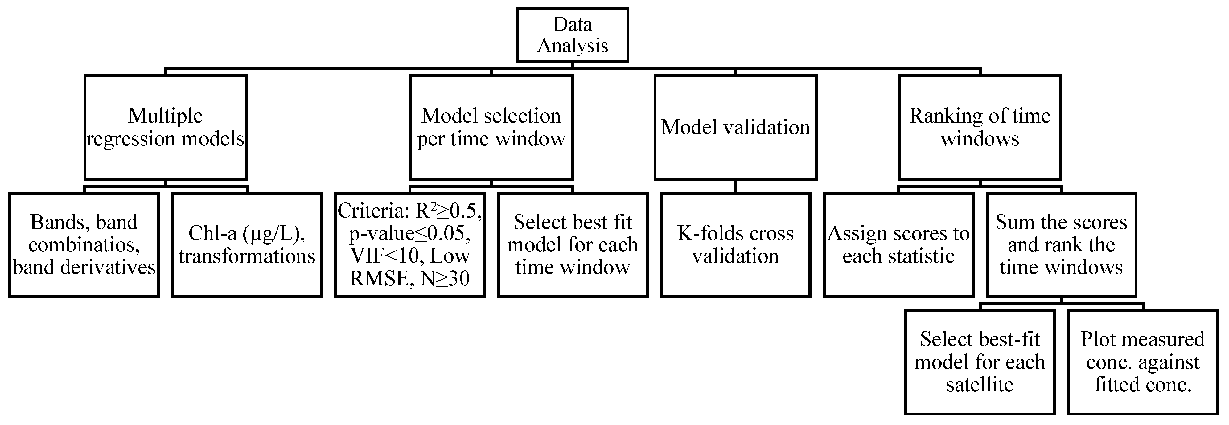
The data analysis followed the following steps that are summarized in Figure 2:
  • Building multiple regression models for each time window;
  • Selection of the best fit model for each time window;
  • Validation of the best fit model for each time window;
  • Ranking of the time windows based on the statistics of their best fit models.

2.4.1. Building and Selection of Best Fit Models

Time windows ranging from ±0 to 5 days were used in the data analysis (Table 1). This 10-day period is the complete cycle for Sentinel-2A and Sentinel-2B. Note that Landsat has a 16-day cycle (eight-day time window); however, only the 5-day time window was used because we did not expect water quality conditions to remain unchanged during the 16-day period due to the dynamic nature of reservoirs in the study area.
Each time window had potentially two or more satellite images from the two acquisition dates (before and after sampling), multiple path/row combinations, or more than one sensor (e.g., Sentinel-2A and Sentinel-2B). When this was the case, the image that included the full extent of the reservoirs under study and the least cloud cover was selected.
Each time window had a pool of data from which a fixed number of samples (15 for Landsat 5, 24 for Landsat 8, and 18 for Sentinel-2) were randomly selected and used in the data analysis. This fixed sample size from each time window was added to those of the preceding time window, thereby increasing the data size as the time window increased. The selection of the fixed amount of data added was dependent on the minimum available data per time window for each satellite.
This incremental data size satisfied the central limit theorem (CLT), which stipulates that the residuals will be closer to the assumed normality when a large data set (N ≥ 30) is used [24]. The sample mean and standard deviation will be closer in value to the population mean (µ) and standard deviation (σ), the larger the sample size. A large sample size also reduces sampling error in the dataset [24].
This study used bands, their combinations, and derivatives following Mansaray et al. (2021). Different spectral bands and band combinations of Landsat 5 TM, Landsat 8 OLI, and Sentinel-2 MSI were used for the development of empirical Chl-a models. The spectral derivative technique [16] was used to obtain first and second-order derivatives for the respective spectral bands of Landsat 5, Landsat 8, and Sentinel-2. These bands, band combinations, and band derivatives were used as independent variables for the multiple regression analysis. The dependent variables were the measured concentrations of Chl-a and two power transformations (the natural logarithm and the square root).
Multiple regression analysis was conducted using the stepwise selection of terms through the forward information criteria (FIC). The FIC involves a step-by-step addition of terms to the regression model. It evaluates how the addition of each term further explains the variation in the dependent variable. The model that gave the best statistics in terms of the coefficient of determination (R2 ≥ 0.5), the significance of the relationship at a 0.05 significance level (p-value (α) ≤ 0.05), minimal multicollinearity of the independent variables (variance inflation factor (VIF) < 10), data size (N ≥ 30), and low root mean square error (RMSE) relative to the concentration range was considered as the best-fit model.

2.4.2. Validation of the Best Fit Models

The best-fit model for each time window was validated using the K-folds cross-validation method. The original sample data was divided randomly into K = 10 subsamples [15,35]. We used Minitab 21 [36] to train the best-fit model using the training set and then tested it using the testing set for each subsample. The R2 and the RMSE were recorded for each round, as shown in the three examples below.
  • Model-1: Trained on Fold-2 + Fold-3 +…. Fold-10; Test on Fold-1; Record R2 & RMSE;
  • Model-2: Trained on Fold-1 + Fold-3 +…. Fold-10; Test on Fold-2; Record R2 & RMSE;
  • Model-10: Trained on Fold-1 + Fold-2 +…. Fold-9; Test on Fold-10; Record R2 & RMSE.
The average R2 and RMSE were used as indicators of the accuracy of the best fit model.
Figure 2 shows a flow chart of the data analysis.

2.4.3. Ranking of the Best Fit Models

The time windows were ranked by R2, RMSE (for both the best fit models and cross-validation), statistical significance (α), data size (N), and VIF. Time windows were highly ranked if they had α ≤ 0.05, R2 ≥ 0.5, RMSE on the low end of the data range, VIF < 10, and N ≥ 30. Each of these criteria was given a score of two (2) if the criterion was satisfied and one (1) if it was not met. The scores were summed to provide a maximum score of 14 and a minimum score of 7. These scores were used to rank the time windows for the reliable pairing of satellite and ground-based data. The model with the time window that had the highest score was selected as the most reliable temporal disparity between satellite spectra and Chl-a data.
Data for each time window were divided into a training and a testing set. The best-fit model was trained and then used to calculate Chl-a concentrations in the testing set using the training data. The fitted Chl-a concentrations were plotted against the measured Chl-a concentrations of the testing set, and the R2 was recorded.

3. Results

3.1. Range of Data

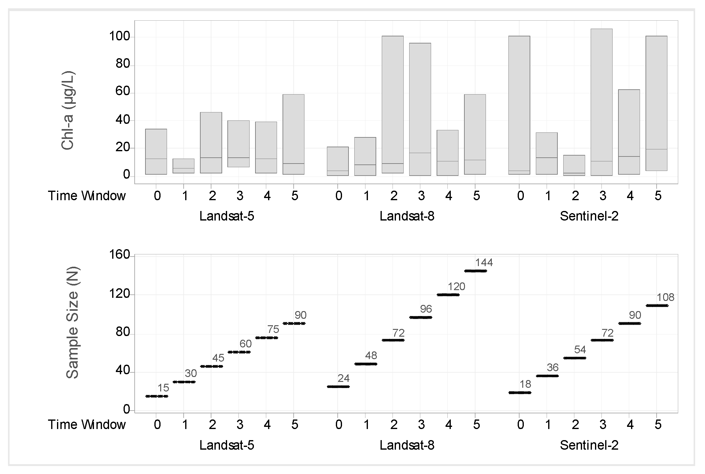
A total of 1371 data points of ground-based Chl-a data were collected in the 10 study reservoirs between 2006 and 2020 (14 years). From this total, there were only 15 data points that were temporally coincident (same day) with a Landsat 5 overpass, 24 with a Landsat 8 overpass, and 20 with a Sentinel-2 overpass. None of the three satellites met the minimum threshold (N = 30) for pairing and development of regression models based on the CLT [23,25]. This observation confirmed the need to expand the time window beyond the same date of image acquisition and ground-based sampling to allow the use of a larger sample size of data points. Figure 3 presents box plots (top panels) showing the minimum, maximum, and median concentrations of Chl-a per time window for the three satellites. In addition, the sample sizes for each time window for the three satellites are shown in the bottom panel of Figure 3.
Chl-a concentrations ranged from 0.62 to 106 µg/L. Landsat 8 and Sentinel-2 had more data points (432 and 333, respectively) than Landsat 5 (197). The two satellites also had higher ranges of data than Landsat 5. The minimum sample sizes for the three satellites were observed in the same-day time window and were 15 for Landsat 5, 24 for Landsat 8, and 18 for Sentinel-2. These minimum sizes became the fixed amount of data that were randomly selected from the pool of data in successive time windows.

3.2. Best Fit Model per Time Window

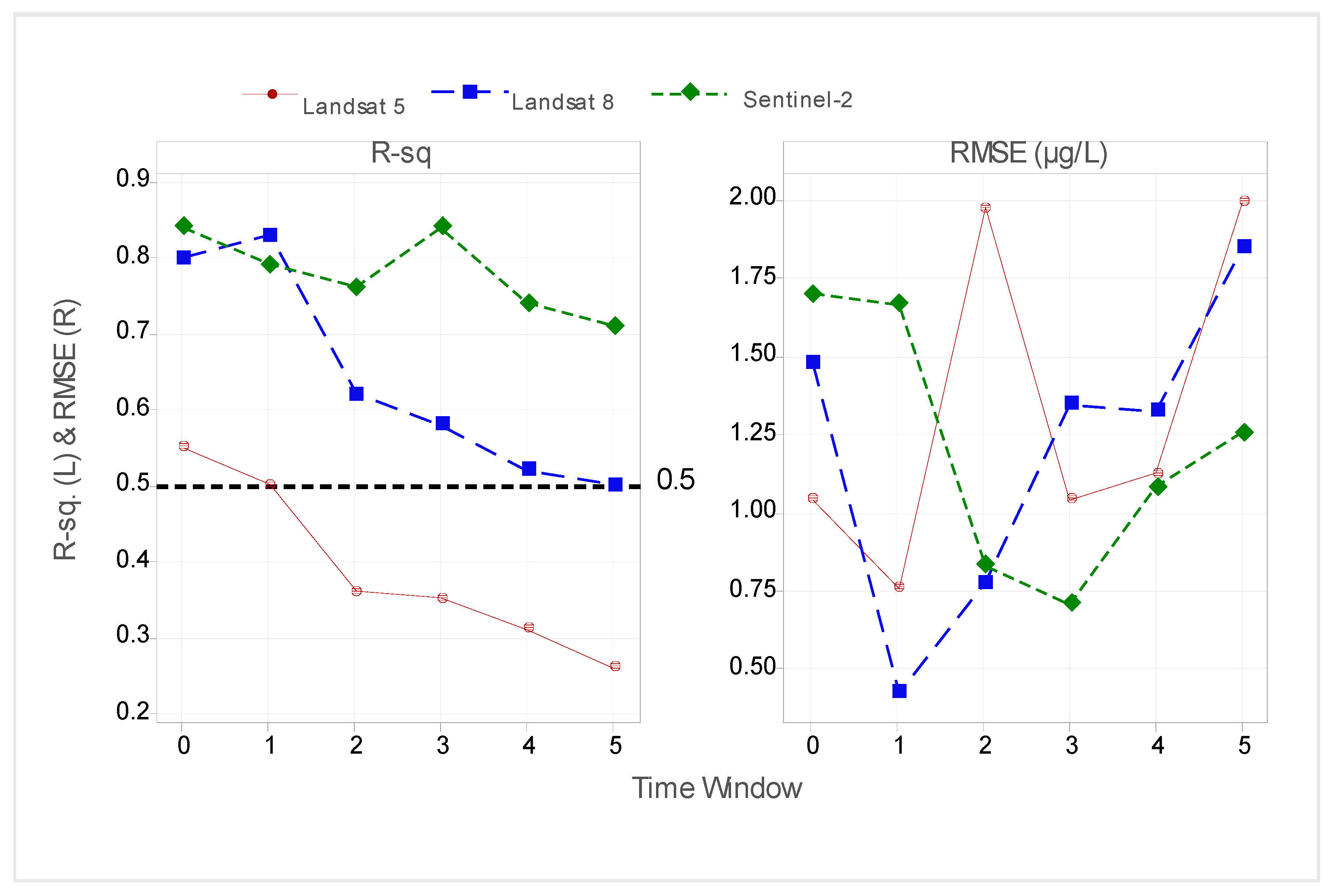
Figure 4 shows the coefficient of determination (R2) and the RMSE for the best fit models per satellite and per time window. In general, the R2 values decreased as the time window increased. Sentinel-2, in general, provided the highest R2 values, followed by Landsat 8 and then Landsat 5.
The highest R2 value for Sentinel-2 (R2 = 0.84) was observed in the temporally coincident (same day) and the 3-day time window. The minimum value (R2 = 0.71) was observed on the 5-day time window. These results reveal that Sentinel-2 spectra can explain at least 71% of the variations in the Chl-a data with temporal disparity up to five days between the overpass and sampling dates.
Landsat 8 spectra explained at least 50% of the variation in data collected up to 5 days before or after image acquisition. The maximum value (R2 = 0.83) was observed in the 1-day time window. The Landsat 8 R2 values were not as high as those for Sentinel-2 after the 2-day window, probably because the lower spatial, spectral, and radiometric resolutions in Landsat 8 contributed to increased uncertainty in the data beyond the 1-day time window.
The Landsat 5 spectra explained at least 50% of the Chl-a data collected within the same day and 1-day time windows only, and the maximum R2 was 0.55 for the day 0 window. These results imply that the spatial, spectral, and/or radiometric resolutions provide advantages of Sentinel-2 and Landsat 8 over Landsat 5 for Chl-a detection in longer time windows between the overpass and sampling dates.
The RMSE values obtained for all the three satellites were all on the low end of the Chl-a concentration range (Chl-a ≤ 2.0 µg/L). The RMSE values ranged from 0.42 µg/L to 1.99 µg/L. The VIF values for all the predictors in the best fit models were also low (VIF < 5). These results confirm the reliability of the best fit models selected for the time windows.

3.3. Validation of the Best-Fit Models per Time Window

Figure 5 shows the average R2 and RMSE values obtained in the 10-folds cross-validation (cv) of the best-fit model for each time window with Landsat 5, Landsat 8, and Sentinel-2.
Sentinel-2 had the highest R2 values, and all its time windows had R2 values greater than the threshold value of R2 = 0.50. For Landsat 8, the R2 threshold up to the 3-day time window (R2 = 0.53), and none of the time windows in Landsat 5 satisfied the R2 threshold (maximum R2 = 0.44). This observation supports the suggestion that higher spatial, spectral, and radiometric resolution satellites are more reliable in pairing data with ground-based Chl-a data considering several days of temporal disparity. The RMSE values were on the low end of the data range for all the sensors and time windows (RMSE ≤ 2.01 µg/L), indicating that considering up to five days of time window, the three satellites can explain variation in Chl-a with minimal error.

3.4. Ranking of the Time Windows Based on Their Respective Statistics

Table 2 presents the ranks of each time window based on the criteria set for the statistics considered in this study (R2 ≥ 0.5; Low RMSE, VIF < 10, N ≥ 30, and α ≤ 0.05). The green rows indicate the time windows that received the maximum score and, hence, the most ideal for pairing the satellite data and their corresponding ground-based data.
The scores indicate that Sentinel-2 spectra can be used to reliably estimate Chl-a data for all the time windows except for the temporally coincident dataset, which had a sample size of less than 30. The Landsat 8 scores imply that sampling should be carried out within three days before or after satellite overpass for reliable algorithm development. The scores in Landsat 5 indicate that the 1-day time window is the most reliable for pairing satellite and ground-based data. These results confirm that the higher the satellite resolution (spatial, spectral, and radiometric), the more reliably their spectra can be used to estimate Chl-a several days before or after image acquisition. Equations (1)–(18) show the best fit models obtained for each time window with Landsat 5, Landsat 8, and Sentinel 2.
Landsat 5
Day 0: SQRT(Chl-a) = 5.96 − 13.93ρd1
Day 1: SQRT(Chl-a) = −1.75 + 4.37ρ(G/R) + 7.79ρd21 + 10.01ρd24
Day 2: LN(Chl-a) = 2.92 + 2.10ρd2 − 3.20ρd23
Day 3: SQRT(Chl-a) = 4.03 − 3.35ρd23
Day 4: SQRT(Chl-a) = 4.08 − 3.23ρd23
Day 5: LN(Chl-a) = 2.77 − 1.68ρ((G-NIR1)/(G + NIR1))2 − 1.53ρd23
Landsat 8
Day 0: Ln(Chl-a) = 6.75 − 76.50ρB − 0.498ρ(R/NIR) − 7.87ρd22
Day 1: SQRT(Chl-a) = 7.95 − 4.66ρ(B/G) − 0.35ρ(R/NIR) + 5.54ρd23
Day 2: SQRT(Chl-a) = 1.86 + 46.80ρd21 + 10.32ρd23 + 20.57ρd25
Day 3: SQRT(Chl-a) = 4.30 + 122.70ρd6 + 69.24ρd21 − 7.90ρd24
Day 4: SQRT(Chl-a) = 6.469 − 3.95ρ(NIR/R) + 56.84ρd21 − 10.93ρd24
Day 5: SQRT(Chl-a) = 7.76 − 5.62ρ(B/G) + 11.23ρd4 + 34.52ρd21
Sentinel 2
Day 0: Ln(Chl-a) = 2.33 + 4.73ρd4
Day 1: Ln (Chl-a) = 2.40 + 4.74ρd4
Day 2: SQRT(Chl-a) = 2.76 + 10.43ρd4 + 11.45ρd7 − 12.70ρd22
Day 3: SQRT(Chl-a) = 2.73 + 10.38ρd4 + 11.47ρd7 − 12.43ρd22
Day 4: SQRT(Chl-a) = 3.09 − 26.94ρRE3 + 9.91ρd4 − 9.30ρd22
Day 5: SQRT(Chl-a) = 8.84 + 1.96ρ((G-NIR)/(G + NIR))2 − 6.09ρ(R/RE1) + 16.76ρd23
Definition of terms
Landsat 5
R = red; G = green; B = blue; NIR = near infrared; MIR = mid infrared; ρ = reflectance; λ = center wavelength; d1 = (G − B)/(λG − λB); d2 = (R − G)/(λR − λG); d3 = (NIR − R)/(λNIR − λR); d4 = (NIR2 − NIR1)/(λNIR2 − λNIR1); d4 = (MIR − NIR2)/(λMIR − λNIR2); d21 = (d2 − d1)/(λR − λB); d22 = (d3 − d2)/(λNIR1 − λG); d23 = (d4 − d3)/(λNIR2 − λR); d24 = (d5 − d4)/(λMIR − λNIR1)
Landsat 8
R = red; G = green; B = blue; NIR = near infrared; SWIR = shortwave infrared; ρ = reflectance; λ = center wavelength; d1 = (B − CA)/(λB − λCA); d2 = (G − B)/(λG − λB); d3 = (R − G)/(λR − λG); d4 = (NIR − R)/(λNIR − λR); d5 = (SWIR1 − NIR)/(λSWIR1 − λNIR); d6 = (SWIR2 − SWIR1)/(λSWIR2 − λSWIR1); d21 = (d2 − d1)/(λG − λCA); d22 = (d3 − d2)/(λR − λB); d23 = (d4 − d3)/(λNIR − λG); d24 = (d5 − d4)/(λSWIR1 − λR); d25 = (d6 − d5)/(λSWIR2 − λNIR)
Sentinel-2
R = red; G = green; B = blue; NIR = near infrared; SWIR = shortwave infrared; RE = red edge; ρ = reflectance; λ = center wavelength; d1 = (B − CA)/(λB − λCA); d2 = (G − B)/(λG − λB); d3 = (R − G)/(λR − λG); d4 = (RE1 − R)/(λRE1 − λR); d5 = (RE2 − RE1)/(λRE2 − λRE1); d6 = (RE3 − RE2)/(λRE3 − λRE2); d7 = (NIR − RE3)/(λNIR − λRE3); d21 = (d2 − d1)/(λG − λCA); d22 = (d3 − d2)/(λR − λB); d23 = (d4 − d3)/(λRE1 − λG); d24 = (d5 − d4)/(λRE2 − λR); d24 = (d6 − d5)/(λRE3 − λRE1)
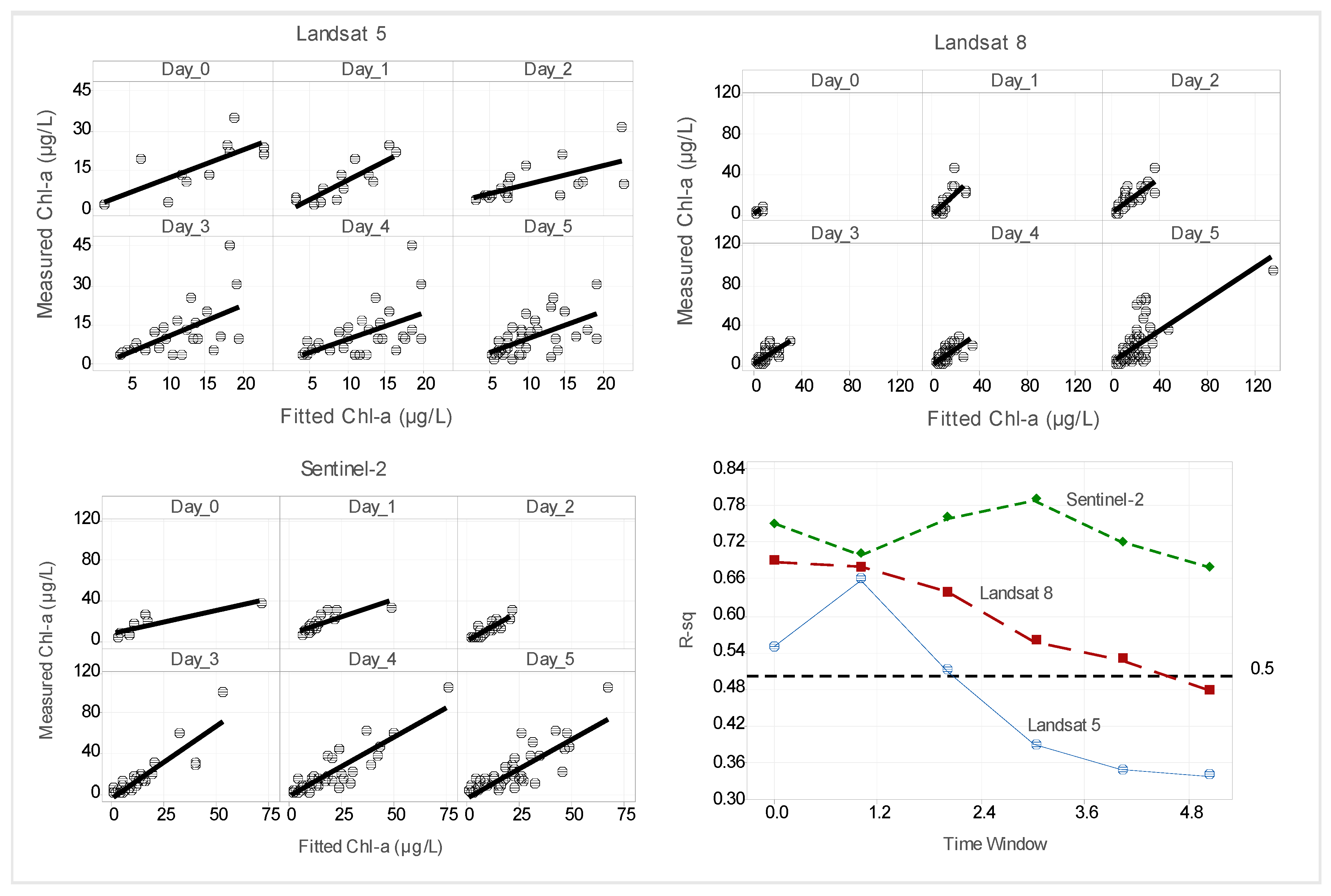
Figure 6 presents scatterplots showing relationships between the Chl-a (µg/L) data predicted by the three satellites and those measured in the study reservoirs for each time window. The R2 values are displayed at the bottom right of the figure. The x-axis represents the measured values, and the y-axis represents the fitted values.
A strong linear relationship was observed between the measured and fitted data for all the time windows in Sentinel-2. For Landsat 8, the 5th day had a linear relationship that did not satisfy the minimum threshold (R2 = 0.5). The strength of the linear relationships in Landsat 5 was below the threshold after day 2.
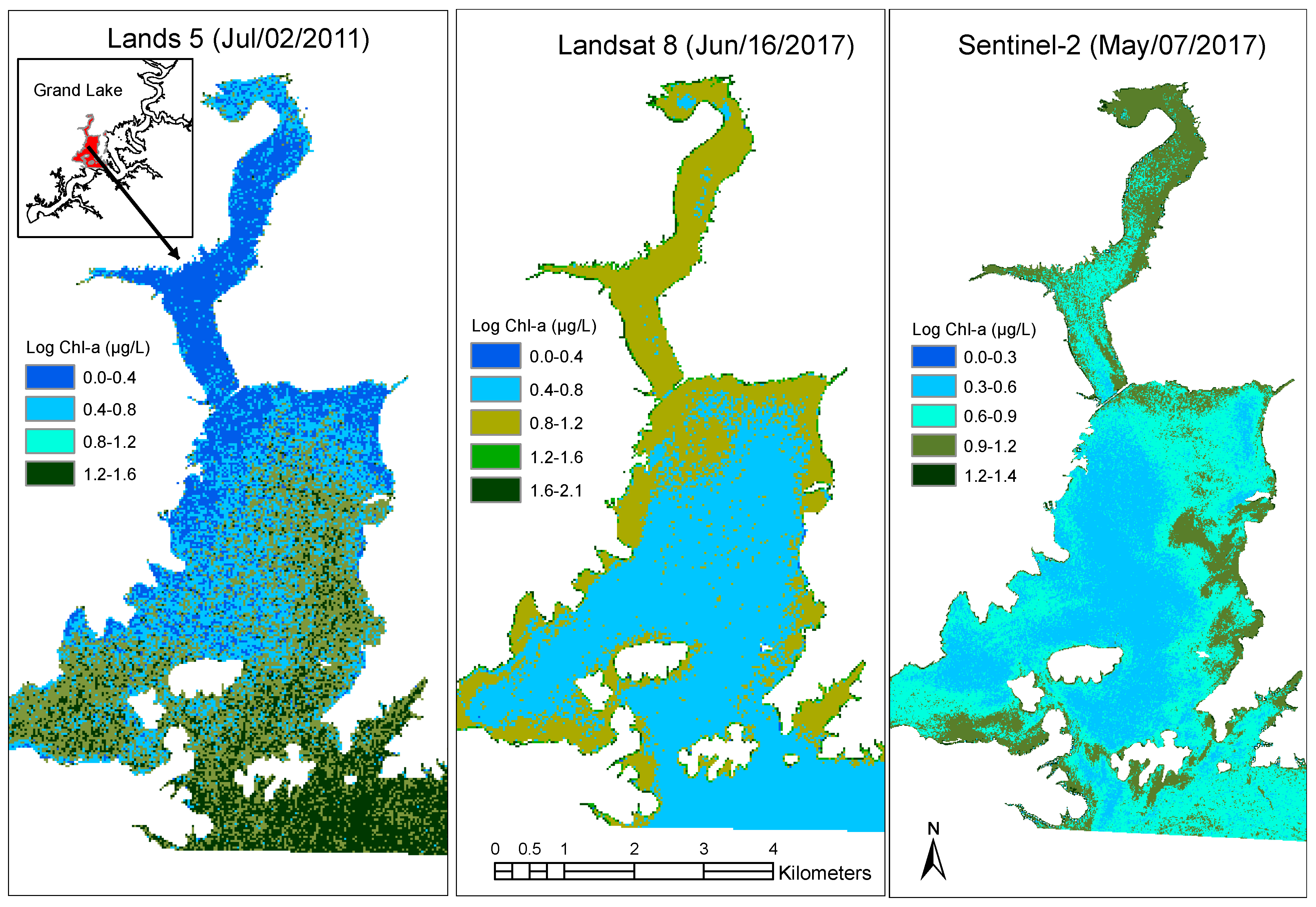
Figure 7 shows Chl-a (µg/L) maps in Horse Creek Cove in Grand Lake, Oklahoma, where algal blooms tend to develop before they spread into the reservoir. The Chl-a maps were developed using Equations (2), (8) and (14) for the 1-day time window with Landsat 5, Landsat 8, and Sentinel-2, respectively. The Landsat 5 image was acquired on 2 July 2011, during a cyanobacterial algal bloom event. The bloom in July 2011 led to an advisory for the public to avoid primary body contact in the reservoir. The Landsat 8 image was acquired on 16 June 2017, and Sentinel-2 on 7 May 2017. Chl-a concentrations as high as 542 µg/L were measured in the edges of the cove during these periods [19].

4. Discussion

Algal blooms have the potential to negatively impact human health and ecosystem function. Chlorophyll-a is present in all major groups of algae and is used as a key indicator of algal blooms in inland water bodies [37]. However, algal blooms are spatially and temporally dynamic in nature, making it challenging to use satellite spectral data to develop algorithms to estimate Chl-a. Understanding how the time window between the satellite overpass and the sample collection impacts algorithm development is an important question when using satellite imagery to assess water quality.
Our study results are consistent with the suggestion that for algorithm development, ground-based data should be collected within a 1-day window before or after the satellite overpass. We also found that Sentinel-2, which has higher spectral, spatial, temporal, and radiometric resolutions than the Landsat satellites, could be paired with ground-based samples up to 5 days before or after overpass. As such, the higher the resolution (spatial, spectral, and radiometric) of the satellite, the longer the temporal window that can be used to develop algorithms with relatively higher R2 values.
For Landsat 5, the highest ranking (13) was observed for the 1-day time window. Increasing the data size across time windows introduced more uncertainty into the Chl-a models. This observation supports Kloiber et al. (2002) that one day of sampling before or after satellite overpass is the most ideal time window to consider for algorithm development. Because R2 values tended to decrease as the time window between the satellite overpass and sampling date increased, we do not support the suggestion that the time window should include more than one day of temporal disparity (e.g., [38]) even if conditions remain the same in the reservoirs under study. This may be different for natural lakes that are not as susceptible to disturbance from the watershed [39].
The strength of the relationship between satellite and ground-based data was observed to be greatest for the 1-, 2-, and 3-day time windows in Landsat 8 (a ranking of 14). This temporal advantage of Landsat 8 over Landsat 5 probably lies in its higher radiometric resolution (16 bits) compared to the latter (8 bits). Landsat 8 has 65,536 (216) brightness values, while Landsat 5 has 256 (28) brightness values. This gives the OLI sensor a higher sensitivity to differences in signal strength compared to the TM sensor [40]. The Landsat 8 result is consistent with Mansaray et al. (2021), who used a two-day temporal disparity for pairing satellite and ground-based data.
The Sentinel-2 results showed that with a higher spatial, spectral, and radiometric resolution, the time window may be increased to five days without introducing significant uncertainty into the model. Many studies have shown that the spatial and spectral advantages of Sentinel-2 make it a better detector of Chl-a than the Landsat sensors [11,15,41,42]. A single Landsat pixel is equivalent to nine Sentinel-2 pixels, which gives its sensor the ability to detect more variations than the Landsat sensors.
Sentinel-2 has 32 bits compared to 16 bits in Landsat 8. This gives Sentinel-2 a total of 232 brightness values, compared to 216 brightness values in Landsat 8 and 28 brightness values in Landsat 5. The presence of specific bands sensitive to Chl-a detection in Sentinel-2 gives it an advantage over Landsat 8 and Landsat 5. The red-edge band effectively interacts with algae at a peak reflectance near 700 nm and is less susceptible to absorption and scattering [11]. Wavelengths in this region have a strong linear relationship with Chl-a [43].
The regression models for the 1-day time window in all three satellites provided strong relationships with the Chl-a data. The band ratios and spectral derivatives (Landsat 5: G/R, d21, d24; Landsat 8: B/G, R/NIR, d23; Sentinel-2: d4) significantly improved the regression models. The ratio of green to red bands positively correlated with Chl-a probably because the pigment reflects green and absorbs red [40]. The negative linear correlations in the B/G and R/NIR bands may be because Chl-a absorbs the blue and red bands [40].
The first derivative, d4, had a positive correlation with the natural log of Chl-a in Sentinel-2. Similarly, the second derivatives d21, d23, and d24 in Landsat 5 and Landsat 8 had a positive correlation with the square root of Chl-a. Studies have shown that spectral derivatives significantly improve regression models for satellite-based water quality detection [14,16].
Overall, all three satellites were shown to estimate Chl-a in the study reservoirs with models derived from data that were paired within varying days of collection per satellite. Sentinel-2 outperformed Landsat 8, which in turn outperformed Landsat 5 in the detection of Chl-a in the incremental time windows. This showed the potential of Sentinel-2 for pairing its spectra with ground-based Chl-a data in reservoirs over a time window of up to 5 days. Landsat 8 can be used for a temporal disparity of up to 3 days. For Landsat 5, however, we may not go beyond the 1-day time window. Sentinel-2 and Landsat 8 can be effectively used in the management of algal blooms and make it easier for lake managers and responsible authorities to take necessary actions to reduce adverse impacts on the environment.

5. Conclusions

Chlorophyll-a is a photosynthetic pigment present in many algal species. It is commonly sampled to determine the severity of algal blooms in water bodies. These blooms may form at times that are missed by ground-based monitoring schedules. Satellite remote sensing has been used to overcome this challenge and increase the monitoring frequency for Chl-a in water bodies.
Our study utilized 14 years (2006–2020) of ground-based Chl-a data for pairing with Landsat 5, Landsat 8, and Sentinel-2′s spectral data to develop multiple regression models. The regression models were developed for six incremental time windows ranging from the same day to five days of sampling before or after satellite overpass—these models utilized surface reflectance from bands, band combinations, and spectral derivatives. The objective was to determine the ideal time window for data pairing and the effect of sensor resolution on the length of temporal disparity.
The study showed that a 1-day time window is ideal for pairing Landsat 5 and ground-based data, up to 3 days for Landsat 8, and up to 5 days for Sentinel-2. This conclusion was drawn based on the criteria of achieving a strong linear relationship between the dependent variable (Chl-a) and the predictors (satellite spectra), the significance of the relationship on a 95% confidence level, minimal uncertainty in the data, and minimal correlation between the predictors. Previous studies have shown that a 1-day time window is ideal with the possibility of extending up to ten days if conditions do not significantly change. Our study adds to this suggestion that it depends on the resolution of the satellite. The higher the spatial, spectral, and radiometric resolution, the more likely it is that we can reliably extend the time window for pairing satellite and ground-based data.
Our conclusion may be limited to human-made reservoirs that constantly receive water flowing from upstream and are generally more variable than natural lakes. Additionally, since the study reservoirs varied in the trophic state (oligotrophic, eutrophic, and hypereutrophic), future research may determine if the effect of the time window differs in reservoirs based on their trophic conditions.
Future research could also include additional determinant parameters, such as hydroclimatic conditions, anthropogenic activities, limnetic mixing, turbidity, oxidation–reduction dynamics, lake water temperature, cumulative sunny days, and precipitation events [10]. Nonetheless, this study provides the basis for selecting a time window between ground-based data collection and satellite overpass for different satellite platforms.

Author Contributions

Conceptualization, P.K.; Data curation, A.S.M.; Formal analysis, P.K. and A.S.M.; Funding acquisition, A.R.D., S.H.S., K.L.W. and A.S.M.; Investigation, P.K.; Methodology, A.R.D., S.H.S. and A.S.M.; Project administration, A.S.M.; Resources, A.R.D., S.H.S. and K.L.W.; Software, A.S.M.; Supervision, A.S.M.; Visualization, A.S.M.; Writing—original draft, P.K.; Writing—review & editing, A.R.D., S.H.S., K.L.W. and A.S.M. All authors have read and agreed to the published version of the manuscript.

Funding

This research was partly funded by the USGS 104b State Water Research Grant, which was awarded by the Oklahoma Water Resources Center, and the APC was funded by Oklahoma State University.

Institutional Review Board Statement

Not applicable.

Informed Consent Statement

Not applicable.

Data Availability Statement

This study did not report data.

Acknowledgments

The authors would like to acknowledge the Oklahoma Water Resources Board for providing the data used in this study. The authors would like to acknowledge the Oklahoma Water Resources Center, Oklahoma State University for partially funding this study.

Conflicts of Interest

There is no conflict of interest.

References

  1. Anderson, D.M.; Glibert, P.M.; Burkholder, J.M. Harmful algal blooms and eutrophication: Nutrient sources, composition, and consequences. Estuaries 2002, 25, 704–726. [Google Scholar] [CrossRef]
  2. Codd, G.A. Toxins of freshwater cyanobacteria. Microbiol. Sci. 1984, 1, 48–52. [Google Scholar] [PubMed]
  3. He, J.; Zhang, Y.; Wu, X.; Yang, Y.; Xu, X.; Zheng, B.; Deng, W.; Shao, Z.; Lu, L.; Wang, L.; et al. A study on the relationship between metabolism of Cyanobacteria and chemical oxygen demand in Dianchi Lake, China. Water Environ. Res. 2019, 91, 1650–1660. [Google Scholar] [CrossRef] [PubMed]
  4. Hudnell, H.K. The state of U.S. freshwater harmful algal blooms assessments, policy and legislation. Toxicon 2010, 55, 1024–1034. [Google Scholar] [CrossRef] [PubMed]
  5. Brooks, B.W.; Lazorchak, J.M.; Howard, M.D.A.; Johnson, M.V.; Morton, S.L.; Perkins, D.A.K.; Reavie, D.E.; Scott, I.G.; Smith, S.A.; Steevens, J.A. Are Harmful Algal Blooms Becoming the Greatest Inland Water Quality Threat to Public Health and Aquatic Ecosystems? Environ. Toxicol. Chem. 2016, 35, 6–13. [Google Scholar] [CrossRef] [PubMed]
  6. Kirk, J. Light and Photosynthesis in Aquatic Ecosystems, 3rd ed.; Cambridge University Press: Cambridge, UK, 2011. [Google Scholar]
  7. Zeng, L.; Li, D. Development of In Situ Sensors for Chlorophyll Concentration Measurement. J. Sens. 2015, 5, 903509. [Google Scholar]
  8. Kuha, J.; Järvinen, M.; Salmi, P.; Karjalainen, J. Calibration of in situ chlorophyll fluorometers for organic matter. Hydrobiologia 2020, 847, 4377–4387. [Google Scholar] [CrossRef] [Green Version]
  9. Gholizadeh, M.H.; Melesse, A.M.; Reddi, L. A Comprehensive Review on Water Qaulity Parameters Estimation Using Remote Sensing Techniques. Sensors 2016, 16, 1298. [Google Scholar] [CrossRef] [Green Version]
  10. Tan, W.; Liu, P.; Liu, Y.; Yang, S.; Feng, S. A 30-Year Assessment of Phytoplankton Blooms in Erhai Lake Using Landsat Imagery: 1987 to 2016. Remote Sens. 2017, 9, 1265. [Google Scholar] [CrossRef] [Green Version]
  11. Bramich, J.; Bolch, C.J.S.; Fischer, A. Improved red-edge chlorophyll-a detection for Sentinel 2. Ecol. Indic. 2021, 120, 106876. [Google Scholar] [CrossRef]
  12. Rodriguez-Lopez, L.; Duran-Llacer, I.; González-Rodríguez, L.; Abarca-del-Rio, R.; Cárdenas, R.; Parra, O.; Martínez-Retureta, R.; Urrutia, R. Spectral analysis using LANDSAT images to monitor the chlorophyll-a concentration in Lake Laja in Chile. Ecol. Inform. 2020, 60, 101183. [Google Scholar] [CrossRef]
  13. Yacobi, Y.Z.; Moses, W.J.; Kaganovsky, S.; Sulimani, B.; Leavitt, C.B.; Gitelson, A.A. NIR-red reflectance-based algorithms for chlorophyll-a estimation in mesotrophic inland and coastal waters: Lake Kinneret case study. Water Res. 2011, 45, 2428–2436. [Google Scholar] [CrossRef] [PubMed] [Green Version]
  14. Han, L. Estimating chlorophyll-a concentration using first-derivative spectra in coastal water. Int. J. Remote Sens. 2007, 26, 5235–5244. [Google Scholar] [CrossRef]
  15. Kuhn, C.; Valerio, A.; Ward, N.; Loken, L.; Sawakuchi, H.O.; Kampel, M.; Richey, J.; Stadler, P.; Crawford, J.; Striegl, R.; et al. Performance of Landsat-8 and Sentinel-2 surface reflectance products for river remote sensing retrievals of chlorophyll-a and turbidity. Remote Sens. Environ. 2019, 224, 104–118. [Google Scholar] [CrossRef] [Green Version]
  16. Becker, B.L.; Lusch, D.P.; Qi, J. Identifying optimal spectral bands from in situ measurements of Great Lakes coastal wetlands using second-derivative analysis. Remote Sens. Environ. 2005, 97, 238–248. [Google Scholar] [CrossRef]
  17. Liu, H.; Lee, S.; Chahl, J.S. Transformation of a high-dimensional color space for material classification. J. Opt. Soc. Am. A 2017, 34, 523–532. [Google Scholar] [CrossRef]
  18. Yan, Y.; Bao, Z.; Shao, J. Phycocyanin concentration retrieval in inland water: A comparative review of the remote sensing techniques and algorithms. J. Great Lakes Res. 2018, 44, 748–755. [Google Scholar] [CrossRef]
  19. Mansaray, A.S.; Dzialowksi, A.R.; Martin, M.E.; Wagner, K.L.; Gholizadeh, H.; Stoodley, S.H. Comparing PlanetScope to Landsat-8 and Sentinel-2 for Sensing Water Quality in Reservoirs in Agricultural Watersheds. Remote Sens. 2021, 13, 1847. [Google Scholar] [CrossRef]
  20. Ouma, Y.O.; Noor, K.; Herbert, K. Modelling Reservoir Chlorophyll-a, TSS, and Turbidity Using Sentinel-2A MSI and Landsat-8 OLI Satellite Sensors with Empirical Multivariate Regression. J. Sens. 2020, 2020, 8858408. [Google Scholar] [CrossRef]
  21. Buma, W.G.; Lee, S. Evaluation of Sentinel-2 and Landsat 8 Images for Estimating Chlorophyll-a Concentrations in Lake Chad, Africa. Remote Sens. 2020, 12, 2437. [Google Scholar] [CrossRef]
  22. Molkov, A.A.; Fedorov, S.V.; Pelevin, V.V.; Korchemkina, E.N. Regional Models for High-Resolution Retrieval of Chlorophyll a and TSM Concentrations in the Gorky Reservoir. Remote Sens. 2019, 11, 1215. [Google Scholar] [CrossRef] [Green Version]
  23. Boucher, J.; Weathers, K.C.; Norouzi, H.; Steele, B. Assessing the effectiveness of Landsat 8 chlorophyll a retrieval algorithms for regional freshwater monitoring. Ecol. Appl. 2018, 28, 1044–1054. [Google Scholar] [CrossRef] [PubMed] [Green Version]
  24. Kloiber, S.M.; Brezonick, P.L.; Olmanson, L.G.; Bauer, M.E. A procedure for regional lake water clarity assessment using Landsat multispectral data. Remote Sens. Environ. 2002, 82, 38–47. [Google Scholar] [CrossRef]
  25. McCullough, I.M.; Loftin, C.S.; Sader, S.A. Combining lake and watershed characteristics with Landsat TM data for remote estimation of regional lake clarity. Remote Sens. Environ. 2012, 123, 109–115. [Google Scholar] [CrossRef]
  26. Brezonik, P.; Menken, K.D.; Bauer, M. Landsat-based Remote Sensing of Lake Water Quality Characteristics, Including Chlorophyll and Colored Dissolved Organic Matter (CDOM). Lake Reserv. Manag. 2005, 21, 373–382. [Google Scholar] [CrossRef]
  27. Urbanski, J.A.; Wochna, A.; Bubak, I.; Grzybowski, W.; Lukawska-Matuszewska, K.; Lacka, M.; Sliwinska, S.; Wojtasiewicz, B.; Zajaczkowski, M. Application of Landsat 8 imagery to regional-scale assessment of lake water quality. Int. J. Appl. Earth Obs. Geoinf. 2016, 51, 28–36. [Google Scholar] [CrossRef]
  28. Keith, D.; Rover, J.; Green, J.; Zalewsky, B.; Charpentier, M.; Thursby, G.; Bishop, J. Monitoring algal blooms in drinking water reservoirs using the Landsat-8 Operational Land Imager. Int. J. Remote Sens. 2018, 39, 2818–2846. [Google Scholar] [CrossRef]
  29. Torbick, N.; Corbiere, M. A Multiscale Mapping Assessment of Lake Champlain Cyanobacterial Harmful Algal Blooms. Int. J. Environ. Res. Public Health 2015, 12, 11560–11578. [Google Scholar] [CrossRef] [Green Version]
  30. Dodds, W.; Whiles, M. Freshwater Ecology: Concepts and Environmental Applications of Limnology, 2nd ed.; (paper back); Academic Press: Amsterdam, The Netherlands, 2010. [Google Scholar]
  31. Boyer, T.A.; Daniels, B.; Melstrom, R.T. Algal Blooms in Oklahoma: Economic Impacts. 2017, pp. AGEC-1063-1–AGEC-1063-2. Available online: https://extension.okstate.edu/fact-sheets/algal-blooms-in-oklahoma-economic-impacts.html# (accessed on 4 January 2022).
  32. Mason, A.M.; Triplett, J.R. Controlling Environmental Crisis Messages in Uncontrollable Media Environments: The 2011 Case of Blue-Green Algae on Grand Lake O’ the Cherokees, OK. In Communicating Cimate-Change and Natural Hazard Risk and Cultivating Resilience: Case Studies for a Multi-Disciplinary Approach; Springer: Cham, Switzerland, 2016; Volume 45, pp. 189–204. [Google Scholar]
  33. OWRB Web Resource. Monitoring and Assessment, Oklahoma Water Resources Board. 2018. Available online: https://www.owrb.ok.gov/quality/monitoring/monitoring.php (accessed on 4 January 2022).
  34. ESA. Copernicus Open Access Hub. European Space Agency. 2022. Available online: https://scihub.copernicus.eu/ (accessed on 2 February 2022).
  35. Kupssinsku, L.S.; Guimaraes, T.T.; de Souza, E.M.; Zanotta, D.C.; Veronez, M.R.; Gonzaga, L.; Mauad, F.F. A Method for Chlorophyll-a and Suspended Solids Prediction through Remote Sensing and Machine Learning. Sensors 2020, 20, 2125. [Google Scholar] [CrossRef] [Green Version]
  36. Minitab. Minitab 21 Support. 2022. Available online: https://support.minitab.com/en-us/minitab/21/?SID=0 (accessed on 2 February 2022).
  37. Topp, S.N.; Pavelsky, T.M.; Jensen, D.; Simard, M.; Ross, M.R.V. Research trends in the use of remote sensing for inland water quality science: Moving towards multidisciplinary applications. Water 2020, 12, 169. [Google Scholar] [CrossRef] [Green Version]
  38. Olmanson, L.G.; Bauer, M.E.; Brezonick, P.L. A 20-year Landsat water clarity census of Minnesota’s 10,000 lakes. Remote Sens. Environ. 2008, 112, 4086–4097. [Google Scholar] [CrossRef]
  39. Kimmel, B.L.; Groger, A.W. Factors Controlling Primary Production in Lakes and Reservoirs: A Perspective. Lake Reserv. Manag. 1984, 1, 277–281. [Google Scholar] [CrossRef]
  40. Jensen, J.R. Introductory Digital Image Processing: A Remote Sensing Perspective, 4th ed.; Pearson: London, UK, 2015. [Google Scholar]
  41. Ansper, A.; Alikas, K. Retrieval of Chlorophyll a from Sentinel-2 MSI Data for the European Union Water Framework Directive. Remote Sens. 2018, 11, 64. [Google Scholar] [CrossRef] [Green Version]
  42. Pereira-Sandoval, M.; Ruiz-Verdu, A.; Tenjo, C.; Delegido, J.; Urrego, P.; Pena, R.; Vicente, E.; Soria, J.; Soria, J.; Morena, J. Calibration and Validation of Algorithms for the Estimation of Chlorophyll-A in Inland Waters with Sentinel-2. In Proceedings of the IGARSS 2018—2018 IEEE International Geoscience and Remote Sensing Symposium, Valencia, Spain, 22–27 July 2018. [Google Scholar]
  43. Gitelson, A.A.; Merzlyak, M.M.; Lichtenthaler, H.K. Detection of Red Edge Position and Chlorophyll Content by Reflectance Measurements near 700 nm. J. Plant Physiol. 1996, 148, 501–508. [Google Scholar] [CrossRef]
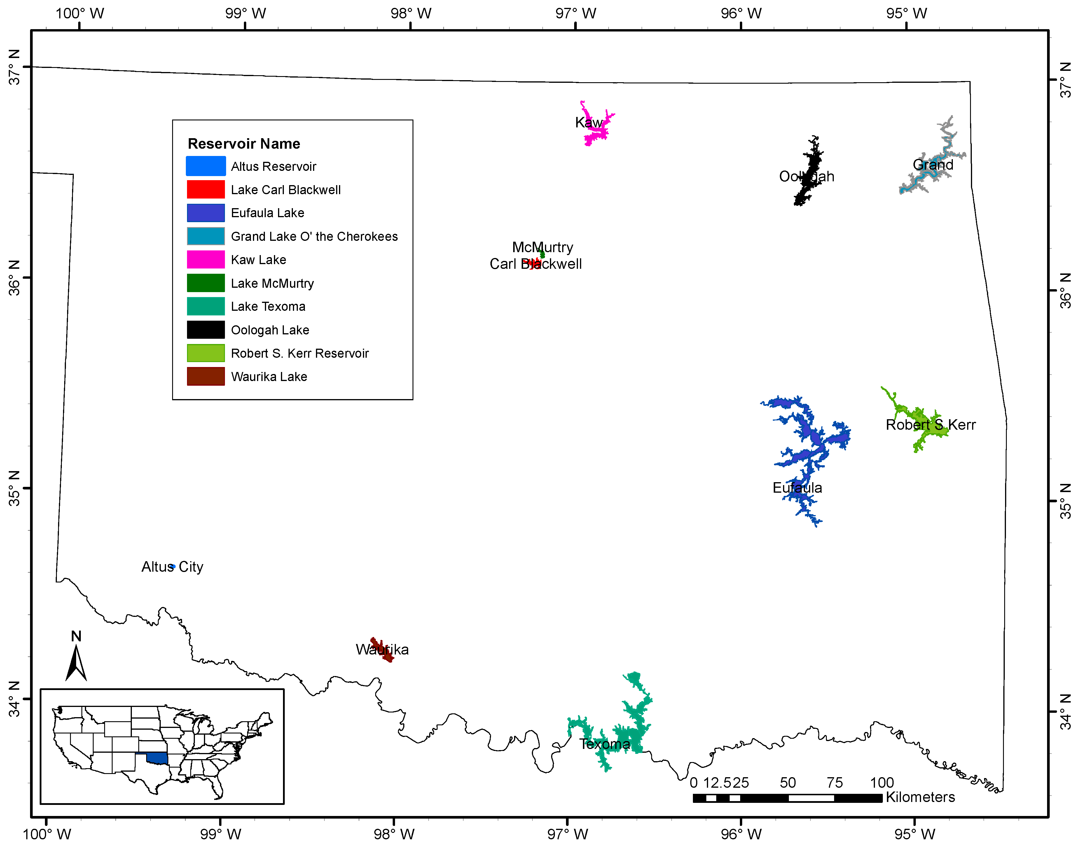
Figure 1. Map of Oklahoma showing the 10 study reservoirs used in this study.
Remotesensing 14 00846 g001
Figure 2. Flow chart summarizing the data analysis.
Remotesensing 14 00846 g002
Figure 3. Minimum, maximum, and median Chl-a concentrations in micrograms per liter per time window (upper panel) and the sample sizes (N) per time window for the three satellites (lower panel).
Remotesensing 14 00846 g003
Figure 4. Graphs of R2 (Left panel) and RMSE (Right panel) for the different time windows and satellites.
Remotesensing 14 00846 g004
Figure 5. Graphs of R2 (Left panel) and RMSE (Right panel) for the 10-fold cross-validation of the models for the different time windows and satellites.
Remotesensing 14 00846 g005
Figure 6. Scatter plots showing the relationships between the fitted concentrations and measured concentrations of Chl-a (µg/L) for the time windows with Landsat 5, Landsat 8, and Sentinel-2. The R2 values are shown at the bottom right of the figure.
Remotesensing 14 00846 g006
Figure 7. Chl-a maps, in log CHL-a (µg/L), in Grand Lake, Oklahoma. The images were taken on different dates by Landsat 5, Landsat 8, and Sentinel-2. The Chl-a concentrations were calculated using Equations (1)–(3) for the 1-day time window with Landsat 5, Landsat 8, and Sentinel 2, respectively.
Remotesensing 14 00846 g007
Table 1. The 5-day time windows utilized in the study.
Time WindowSampling before Satellite OverpassSame Day Sampling after Satellite Overpass
0 0
1 −101
2 −2−1012
3 −3−2−10123
4 −4−3−2−101234
5−5−4−3−2−1012345
Table 2. Ranking of the time windows for each satellite based on selected statistics. The green rows indicate the time windows that received the maximum score.
Time WindowR2RMSER2 (cv)RMSE (cv)VIFSignificanceNScore
Landsat 50221222112
1221222213
2121222212
3121222212
4121222212
5121222212
Landsat 80222222113
1222222214
2222222214
3222222214
4221222213
5221222213
Sentinel-20222222113
1222222214
2222222214
3222222214
4222222214
5222222214
Publisher’s Note: MDPI stays neutral with regard to jurisdictional claims in published maps and institutional affiliations.