Abstract
Yunnan province in China has rich forest resources but high forest fire frequency. Therefore, a better understanding of the relationship between climate change and forest fires in this region is important for forest fire prevention. This study used the Gravity Recovery and Climate Experiment (GRACE) terrestrial water storage change (TWSC) data to analyze the influence of climate change on forest fires in the region during 2003–2016. To improve the accuracy and reliability of GRACE TWSC data, we used the generalized three-cornered hat (GTCH) and the least square method to fuse TWSC data from six GRACE solutions. The spatiotemporal variation of forest fires during 2003–2016 was investigated using burned area data. Then, the relationship between burned area and hydrological and climatic factors was analyzed. The results indicate that more than 90% of burned areas are located in northwestern and southern Yunnan (NW and S). On the seasonal scale, forest fires are mainly concentrated in January–April (dry season) and the burned area is negatively correlated with precipitation (correlation coefficient r = −0.83 (NW) and −0.51 (S)), relative humidity (r = −0.79 (NW) and −0.92 (S)), GRACE TWSC (r = −0.57 (NW) and −0.73 (S)) and evapotranspiration (r = −0.90 (NW) and −0.35 (S)). However, the burned area has no significant correlations with the above four factors on the interannual scale. The composite analysis suggests that the extreme climate affects precipitation, evapotranspiration and TWSC in this region, thereby changing water storage of the air in this region, leading to the formation of an environment prone to forest fires. Such conditions have led to an increase in the burned area in the above region. We also found that the difference between TWSC in high- and low-fire years is much greater than the precipitation in the same period. The above results show that GRACE satellites can detect the influence of climate change on forest fires in Yunnan province.
1. Introduction
Forest fires are serious natural disasters, which have caused enormous damage to human society, ecological environments and economic development [1]. According to statistics, there were more than 139,000 forest fires in North America each year, with a total area of 4.2 million hm2 [2]. In 2019, the Amazon rainforest fire continued to burn for more than 21 days, and the burned area exceeded 1 million hm2. It has caused serious damage to the local ecological environment and may be a greater influence on the local and global climate [3]. During 2019–2020, the wildfire in Australia killed at least 33 people and about 1 billion animals, and the affected area was more than 10 million hm2. The heavy smoke caused by the wildfire lasted for several weeks and blocked many cities including Sydney, and the local ecological environment was severely damaged [4]. Therefore, it is of great significance to study the driving factors of forest fires for effectively controlling the occurrence of forest fires.
Forest fire occurrence is driven by many factors including weather condition [5], human activities [6], fuel characteristics [7], fire management [8], land use changes [9] and climate changes [10,11]. Among these, climate change is a key factor contributing to forest fires [12,13], which mainly affects forest fires in two ways. On the one hand, climate change affects the occurrence of forest fires by changing the dryness of combustibles through temperature, precipitation (PPT), evapotranspiration (ET), etc. [14,15,16]. On the other hand, climate change can change the composition, properties and biomass of combustibles by affecting the structure and growth of vegetation, which affects the behavior of forest fires [17,18,19]. Swetnam et al. [20] and Jones et al. [21] indicate that the large-scale climate model of Pacific Decadal-scale oscillations and strong El Niño/La Niña events is closely related to the frequency and severity of forest fires. The severity of forest fires has a certain correlation with abnormal ocean surface temperature and Palmer Drought Severity Index [5,22,23]. Gillett et al. [24] indicate that the increase in the area of burned areas in Canada from 1920 to 1990 is related to the trend of regional warming over the same period. Heyerdahl et al. [25] explain that the frequency of forest fires in inland forests is synchronized with the changes in the dry and wet climates in spring and summer. Westering et al. [26] analyzed the influence of climate change in the western United States on forest fires. The results show that the increase in average temperature and the extension of dry periods have increased the number of forest fires in the western United States by nearly three times, and the burned area has increased by nearly six times. Pausas et al. [27] studied the relationship between climate change and forest fires in the Iberian Peninsula from 1950 to 2000. The results show that the summer temperature and PPT are significantly related to the frequency of forest fires and the fire area in the same period.
In 2002, the Gravity Recovery and Climate Experiment (GRACE) was implemented to detect the changes of Earth’s gravity field on medium and long scales [28]. These changes mainly come from terrestrial water, so it is generally considered that Earth’s surface mass changes detected by GRACE are equivalent to terrestrial water storage change (TWSC) [29]. As an important part of the regional water cycle, TWSC can not only reflect the water balance relationship between water inputs (such as, PPT, snowfall, etc.) and water outputs (such as runoff, ET, etc.) but also was used to evaluate the influence of climate change on regional hydrological changes [30,31]. Therefore, it is feasible to use GRACE TWSC to study the influence of climate change on forest fires.
Yunnan province is one of the major forest regions and the most frequent and hardest-hit region of forest fires in China [32]. There is high forest coverage rate and rich forest resources. Forest fires in this region are characterized by a long fire-prevention period, complex terrain and difficulty in fighting the fires. During 1996–2008, there were 135.8 thousand forest fires that occurred, 0.1358 million hm2 of forest burned, 67 people died from fighting fires and 142 people were burned [33]. Yunnan is located on a plateau with complex topography; there are significant regional differences and vertical changes in climate, and regional climate changes are inconsistent [32]. Therefore, studying the relationship between forest fires and climate change will help to scientifically understand the laws of temporal and spatial changes of forest fires in this region, and provide scientific data support for government departments’ forest fire prevention and macro decision making.
However, there are few studies about using GRACE TWSC to detect the influence of climate change on forest fires [34,35]. In particular, research about Yunnan province has not been reported in the literature to the best of our knowledge. Due to the differences between different GRACE solutions, it may lead to unreliable results [36]. Therefore, we first used the generalized three-cornered hat method (GTCH) to evaluate the uncertainly of six GRACE solutions in this paper, then the least squares method was used to integrate the TWSC results from the above GRACE solutions. Moreover, the fusion result was used to investigate the climatic characteristics of Yunnan province. Finally, the connection between climate change and forest fires was analyzed. This paper is organized as follows. In Section 2, Section 3 and Section 4, the study area, data and study methods are introduced separately. Section 5 presents the spatial and temporal distribution of fire burned area, the climate change characteristics in Yunnan and the analysis results of the influence of climate change on forest fires. The discussion and conclusion are provided in Section 6 and Section 7, respectively.
2. Study Area
Yunnan is located in Southwest China, approximately at 21°–30°N and 97°–106°E, with a total area of about 390,000 km2 (see Figure 1). This region is a mountainous plateau region: most of the region is mountainous, and the overall terrain tends to be higher in the west and lower in the east [32]. Warm in winter and cool in summer, all seasons are like spring. There are also complex vegetation types and rich forest resources in this region. Because it is located at the intersection of frigid and tropical zone plant regions, plants of the frigid, warm and hot zones have grown. In addition, the distribution of vegetation in this region has obvious horizontal zonality. From north to south, the vegetation types are cold-temperate coniferous forest, subtropical semi-humid evergreen broad-leaved forest, subtropical monsoon evergreen broad-leaved forest, tropical monsoon forest and tropical rainforest [37].
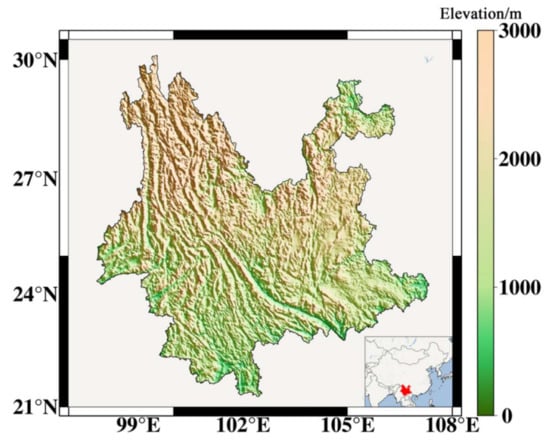
Figure 1.
Digital elevation model of Yunnan.
3. Data
3.1. GRACE Data
To obtain monthly 1° × 1° gridded TWSC data, we used four GRACE RL06 spherical harmonic (SH) solutions provided by the Center for Space Research at the University of Texas at Austin (CSR), Helmholtz–Centre Potsdam–German Research Centre for Geosciences (GFZ), Jet Propulsion Laboratory (JPL) and Institute of Geodesy at Graz University of Technology (ITSG), respectively. Before calculating the gridded TWSC data, we needed to perform several types of preprocessing on the four SH solutions. Firstly, C20 of SH coefficients have been replaced with those of satellite laser ranging [38]. The degree-1 coefficients have been replaced using the results from Swenson et al. [39]. To minimize the effects of high-frequency and correlated errors, the combined filtering (300 km Fan filter and de-striping method P3M6) has been applied for smoothing the SH solutions [40]. To reduce the signal attenuation effect caused by order truncation and filter smoothing, the GRACE TWSC data was corrected by using the scale factor approach [41].
In this study, we also obtained the monthly 1° × 1° global gridded TWSC data derived from two Mascon solutions provided by CSR and JPL. The JPL Mascon is Release 06 Version 1.0 with the coastal resolution improvement filter [42], and the CSR Mascon is Release 06 Version 2.0 [43]. Unlike SH solutions, Mascon solutions do not require additional processing and can be directly read and used. A number of measures have been taken to improve the accuracy of Mascon solutions. Firstly, the C20 coefficients have been replaced with the solutions from SLR. Secondly, the degree-1 coefficients have been estimated using the results of TN-13a [44] and the approach of Sun et al. [45] and Swenson et al. [39]. Thirdly, the ice rebound correction has adopted ICE6G-D model [46].
Therefore, the four SH solutions and two Mascon solutions were used to obtain monthly GRACE TWSC gridded data in Yunnan from January 2003 to December 2016 in this study. For convenience, the four SH solutions and two Mascon solutions are termed CSR-SH, GFZ-SH, JPL-SH, ITSG-SH, CSR-M and JPL-M.
3.2. Burned Area Data
The monthly global gridded burned area data from January 2003 to December 2016 was provided by the Global Fire Emission Database Version 4.1s (GFED4.1s) [47,48] in our study, which was used to estimate the fire-affected area during forest fires in Yunnan. The GFED4.1s product is a collection of multiple satellite detection data, including the Moderate-resolution Imaging Spectroradiometer (MODIS), the Tropical Rainfall Measuring Mission (TRMM) Visible and Infrared Scanner (VIRS) and the Along-Track Scanning Radiometer (ATSR) family of sensors [49]. This database with spatial resolution 0.25° × 0.25° provides four components: burned area, carbon emissions, biosphere fluxes and other ancillary data sets.
3.3. In Situ PPT Data
The monthly gridded PPT data with spatial resolution 0.5° × 0.5° from January 2003 to December 2016 was provided by the China National Meteorological Science Data Center in our study. The datasets come from the monthly PPT data at national-level stations nationwide from 1961 to the present, which were collected and compiled by the China National Meteorological Information Center.
3.4. Evapotranspiration (ET) Data
We used the ET gridded data with spatial resolution 0.25° × 0.25° from January 2003 to December 2016 derived from the Global Land Evaporation Amsterdam Model (GLEAM) 3.5a [50,51] in our study. The model is a set of algorithms that separately estimate the different components of land evaporation: transpiration, bared-soil evaporation, interception loss, open-water evaporation and sublimation. Additionally, GLEAM provides surface and root-zone soil moisture, potential evaporation and evaporative stress conditions.
3.5. Relative Humidity Data
To further investigate the relationship between humidity changes in air and forest fires, we used the relative humidity gridded data derived from the National Centers for Environmental Prediction-Department of Energy (NCEP-DOE) Reanalysis 2 project. The data are provided by Physical Sciences Laboratory at the National Oceanic and Atmospheric Administration (NOAA). The NCEP-DOE Reanalysis 2 project is using a state-of-the-art analysis/forecast system to perform data assimilation using past data from 1979 through the previous year [52], and the temporal coverage of the data are 4-times daily, daily and monthly. In our study, we used the monthly relative humidity gridded data with spatial resolution 2.5° × 2.5° from January 2003 to December 2016.
3.6. Atmospheric Column Water Vapor
To investigate the role of water storage in regulating air and fuel moisture, the global atmospheric column water vapor monthly gridded observations with spatial solutions 1° × 1° were used in our study, which are derived from the Atmospheric Infrared Sounder (AIRS) [53]. In our study, the monthly atmospheric column water vapor gridded data were used from January 2003 to December 2016.
3.7. Extreme Climate Index
Since PPT and ET of Yunnan are affected by the El Niño-Southern Oscillation (ENSO) and the Indian Ocean Dipole [40,54], we included the above two extreme climates into the analysis scope when studying the influence of climate change on forest fires in Yunnan. The monthly Niño 3.4 index data indicate the magnitude of ENSO, which is provided by the National Oceanic and Atmospheric Administration (NOAA). The Indian Ocean Dipole Model Index (DMI) is defined as the difference in the average sea surface temperature anomaly between the Tropical Western Indian Ocean and the Equatorial Southeast Indian Ocean [55]. The monthly DMI data were also provided by NOAA. The above index data in our study are from January 2003 to December 2016.
4. Method
4.1. Fusing Different Datasets
Due to discrepancies in different GRACE TWSC datasets, inconsistent results may appear, which may confuse the analysis results. Hereafter, to minimize the discrepancies caused by different datasets and improve the reliability of the results, we used the GTCH method to estimate the relative uncertainties of the six GRACE TWSC datasets, and fused them according to their uncertainties using the least square method.
4.1.1. The GTCH Method
This method can estimate relative covariances of different datasets without a priori knowledge as long as there are at least three datasets [56,57]. Suppose there are several different observation series, denoted by , correspond to different data. Each observation series can be expressed as:
where is the real signal, is the error of the observation series (0 means white noise) and N is the number of observation series. Since the true signal cannot be obtained, any observation series was selected as the reference signal, and the choice of the reference series does not influence the final results [58]. Then, the difference series between the remaining observation series and the reference series was calculated [59].
where is the reference observation series and is the errors of reference observation series. The TWSC series derived from the JPL Mascon solution was selected as the reference series. N − 1 difference series were stored in the following matrix.
where M is the number of observations in the series. The covariance matrix of difference series is:
where is the covariance operator. is the variance estimate or covariance estimate , that is, the variance or covariance estimate of difference series between the TWSC series derived from different GRACE solutions and the reference series. The unknown noise covariance matrix R was introduced, and its relationship with S is [60]:
where the matrix J is:
The matrix R is:
From Equation (5), the following relationship can be obtained:
Both R and S are real symmetric matrices by definition. There are unknown parameters for R, but there are only equations for S. Therefore, Equation (5) is underdetermined. As a results, the remaining free parameters need a reasonable way to obtain a unique solution [60].
To guarantee the positive definiteness of R, Galindo and Palacio [61] proposed an important constraint on the solution space for free parameters based on the Kuhn–Tucker theorem.
where , which is introduced for a better numerical solution. is given by [62]:
This condition constrains the free parameters in the solution domain, but it is still not enough to obtain the unique solution of the free parameters [59]. It is necessary to give the optimal selection criteria to obtain the unique parameter solution. Tavella and Premoli [58] proposed that the determination of the free parameters is based on the minimum “global correlation” of all observation series and the positive definiteness of R. Therefore, the following objective function was defined and minimized to determine the free parameters [61].
In order to make the initial value within the constraints, the initial value of the iterative calculation was set to [58]
Minimize the objective function (Equation (11)) to obtain a set of free parameter solutions under constraints (Equation (9)), that is, the variance of the uncertainty of different observation series. Other unknown elements in R can be obtained by Equation (8).
4.1.2. Data Fusion
We applied the GTCH method to estimate the relative covariance of TWSC derived from six GRACE datasets. Then we fused the six TWSC results by taking a weighted average of them [44].
where and are the TWSC results derived from the individual GRACE solution and its corresponding weight, respectively. The weights were determined based on estimated variances.
where is the variance of the th TWSC time series estimated by the GTCH method. The above process was performed grid by grid until we fused the six datasets on all the grid nodes.
4.2. Composite Analysis
In the climate change research, composite analysis was used to explore the salient characteristics of certain special years [63]. In our study, we first standardized the time series of burned area. Then, the special years were selected according to the rule of greater than 0.5 times or less than 0.5 times the standard deviation based on the standardized time series of burned area, which were marked as high- and low-burned area years, respectively. Finally, the average of meteorological and hydrological elements of these special years were compared with the ones of all years to analyze the difference of these elements during high- and low-burned area years.
4.3. Pearson Correlation Analysis
In our study, we used the Pearson correlation analysis to evaluate the relationship between two sets of data. In statistics, the covariance of two sets of data is generally divided by the standard deviation of the corresponding data series to obtain the Pearson correlation coefficient [4]. For and two sets of time series, the Pearson correlation coefficient can be estimated by the following expression:
where is the number of observations in the time series and . and are the average values of the time series and during the study period. The value range of is between −1 and 1.
4.4. Time Series Analysis
The time series of observation signals contains the long-term change trend, acceleration, seasonal change (annual change and semi-annual change) and residual signal. The corresponding signals can be extracted from the linear fitting model. The decomposition is expressed as follows [64,65]:
where is the time series of TWSC; is the time; is the midpoint of the entire research period; is the error and other signal; and , , , , , and are the unknown parameters. is constant term, is long-term trend change, is the acceleration, and are annual terms and and are semi-annual terms.
5. Results
5.1. GRACE Solutions Fusion
Figure 2 shows the spatial distribution of uncertainties of six GRACE-based TWSC results estimated by the GTCH method in Yunnan. It can be seen that the uncertainties of TWSC results derived from the four SH solutions are smaller than those of two Mascon solutions. Specifically, the uncertainties of TWSC results from the four GRACE SH solutions are smaller than 4 cm, while TWSC results from the two GRACE Mascon solutions show uncertainties greater than 4 cm in most regions. Except for GFZ-SH, the regions with greater uncertainty are mainly concentrated in western Yunnan. Specifically, the uncertainty of TWSC results from two GRACE Mascon solutions are higher than 6 cm in the above region.
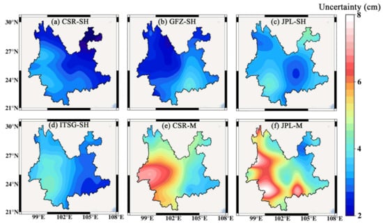
Figure 2.
The spatial distribution of uncertainties of TWSC results derived from CSR-SH (a), GFZ-SH (b), JPL-SH (c), ITSG-SH (d), CSR-M (e) and JPL-M (f) solutions estimated by the GTCH method.
To evaluate the overall uncertainty of six GRACE solutions, we sorted the grid values of certainty in the study region in ascending order and took the median one to represent the overall uncertainty in this region. The results are presented in Table 1. The six GRACE solutions were sorted in ascending order of the uncertainty of TWSC results, and their arrangement is GFZ-SH (2.63 cm), CSR-SH (2.66 cm), ITSG-SH (3.02 cm), JPL-SH (3.40 cm), JPL-M (4.62 cm) and CSR-M (5.11 cm). It can be seen that the results of GFZ-SH and CSR-SH are very close. In our study, we estimated only the relative accuracy. If you want absolute accuracy, you need ground truth data.

Table 1.
Uncertainties of TWSC results derived from six GRACE solution and fusion result estimated by the GTCH method.
Based on the variances of six GRACE-based TWSC results estimated by the GTCH method, we fused these six results to yield the fused results. From Table 1, we found that the uncertainty of the fusion result is much smaller than the ones of six single solutions. Figure 3 shows the spatial distribution of uncertainties of the fusion result. Comparing Figure 2 and Figure 4, we found that all the uncertainties of fusion result are lower than 1.5 cm, while the ones of six single solutions are all higher than 2 cm. This suggests that the accuracy of the fusion result has been significantly improved.
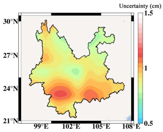
Figure 3.
The spatial distribution of uncertainties of TWSC results derived from fusion model.
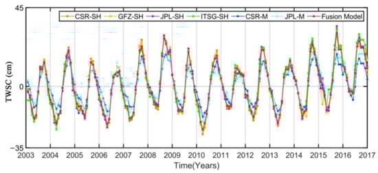
Figure 4.
The time-series of TWSC derived from six GRACE solutions and fusion results.
Figure 4 shows the time series of TWSC results derived from six GRACE solutions and the fusion result in the study region. It can be seen that TWSC time series from six GRACE solutions and the fusion result have the similar magnitude. However, the magnitudes of TWSC time series from Mascon solutions are smaller than the ones from SH solutions. The fusion result is close to the TWSC results from SH solutions, because the uncertainties of the TWSC results from SH solutions are smaller than the ones of Mascon solutions, so the weights of SH solutions are larger than the ones of Mascon solutions in the fusion process. To further evaluate the fusion result, we calculated the correlation coefficients between the fusion result and the TWSC results from six single solutions (see Table 2). From Table 2, among six solutions, the correlation coefficient between the fusion result and CSR-SH is the highest (0.9968), followed by GFZ-SH, JPL-SH, ITSG-SH and CSR-M. The smallest one is JPL-M (0.9741). Therefore, the similar magnitude and high correlation suggest that the fusion result has good consistency with TWSC results from six GRACE solutions.
Table 2.
The correlation coefficients between fusion results and TWSC results from six GRACE solutions.
5.2. Spatial and Temporal Distribution of the Burned Area
Figure 5 shows the spatial distribution of monthly average burned area from 2003 to 2016 across Yunnan. From the figure, we found that the forest fires were mainly concentrated in northwest (NW), southern (S) and central Yunnan. Among the three regions, the region with the longest forest fire duration and the largest accumulation of burned area is region NW, followed by region S, and finally the central region. In region NW (25°–30°N and 97°–101°E), the high-fire months are February, March, October, November and December and the burned areas in most regions are larger than 18 ha, while the low-fire months are August and September and the burned areas in this region are smaller than 4 ha. In region S (21°–24°N and 98°–104°E), the high-fire months are February, March, April and December and the burned areas in most regions are larger than 4 ha, while the low-fire months are May, June, Auguest and October and the burned areas in most regions are smaller than 4 ha. There were no fires in June or October. In the central region, the forest fires only appeared in March, April and May. The largest burned area occurred in April. Except for the above three regions, there are fewer forest fires in other regions, and forest fires are mainly concentrated in region NW and S. The burned area in region NW is larger than the one in region S. Therefore, we focused on the above two regions in the following research.
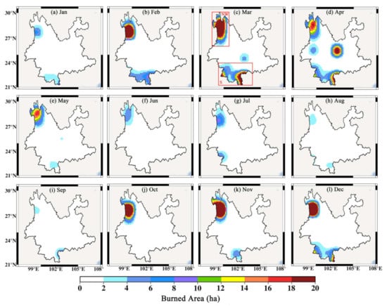
Figure 5.
The spatial distribution of the monthly burned area averaged from 2003–2016 across Yunnan. (a–l) represent the results from January to December, respectively. (NW: Northwestern; S: Southern).
Figure 6 shows the monthly average burned area during 2003–2016 in Yunnan, regions NW and S, and the percentages of burned area of regions NW and S divided by the ones in Yunnan. The maximum monthly average burned area (85,446 ha) and the minimum one (4110 ha) in Yunnan appeared in March and September, respectively; forest fires are mainly concentrated in winter and spring (January, February, March and April). The monthly burned areas in the high-fire months are more than 50,000 ha, which are much higher than those of other months. The maximum and minimum monthly burned areas in region NW appear in January and September, respectively; forest fires are mainly concentrated in autumn and winter (November, December, January and February). The monthly burned areas in these high-fire months are higher than 20,000 ha, while the ones in other months are lower than 14,000 ha. The largest proportion of burned area (82.06%) occurs in November, and the smallest one (13.15%) occurs in April. The average is 48.03%. In region S, the maximum monthly burned area appears in March, while the minimum one appears in September and October; forest fires are mainly concentrated in winter and spring (February, March and April). The monthly burned areas in these high-fire months are higher than 11,000 ha, while the ones in other months are lower than 5000 ha. The largest proportion of burned areas in Yunnan (26.25%) occurred in March, and the smallest one (3.16%) occurred in November. The average value is 12.62%.
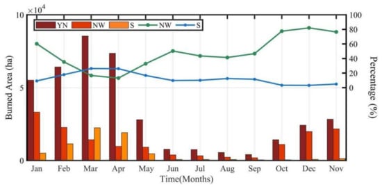
Figure 6.
The monthly average of burned area from 2003–2016 for Yunnan (scarlet, YN), region NW (light red) and S (Orange) and the percentage of monthly average burned area of region NW and S in the one of Yunnan (green line: NW, blue line: S).
According to the above numerical results, the low-fire months in the three regions are June, July, August and September. However, there is a significant difference between region NW and other two regions in the high fire months. Except for region NW, the temporal distribution of burned areas in Yunnan and region S are similar on the seasonal scale. This may be because region NW belongs to part of the Qinghai–Tibet Plateau. Therefore, its climatic characteristics are quite different from other parts of Yunnan [33]. According to the results of burned area percentage, it can be seen that regions NW and S are the regions that are more prone to forest fires in Yunnan, which is consistent with the results of Figure 5.
Figure 7 shows the temporal evolution of annual burned area for the period 2003–2016 in Yunnan, regions NW and S. According to composite analysis, the high and low burned years in three regions were determined. In Yunnan, the high-fire years are 2004, 2005, 2006, 2007 and 2009, while the low ones are 2008, 2012, 2014 and 2016. In region NW, 2003, 2006, 2007, 2009 and 2010 are the high-fire years, and 2004, 2008, 2011, 2012, 2013 and 2016 are the low fire years. In region S, the high-fire years are 2004, 2006, 2009, 2011 and 2015, while the low ones are 2007, 2008, 2010, 2012, 2014 and 2016.
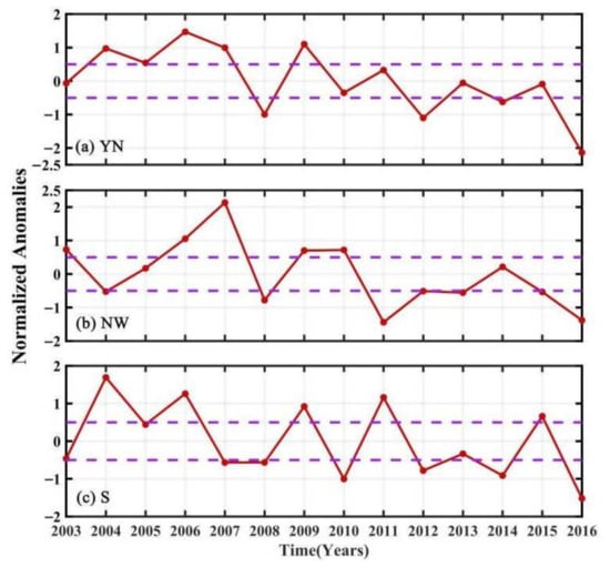
Figure 7.
The temporal evolution of annual burned area normalized anomalies (red solid line) for the period of 2003–2016 in Yunnan (a), region NW (b) and S (c). The purple dashed line denotes the ±0.5 standard deviation. The normalized anomalies mean that the time series of burned area was standardized.
Comparing Figure 7a–c the common high-fire years of three regions are 2006 and 2009, while the common low-fire years are 2012 and 2016. It can be seen that the interannual variation of forest fires in Yunnan is different from those in regions NW and S. Comparing Figure 7b,c, the common high-fire years of region NW and S are 2006 and 2009, while the common low-fire years are 2008, 2012 and 2016. 2004, 2011 and 2015 are the low-fire years in region NW, but they are the high-fire years in region S. 2010 is the high-fire year in region NW, but it is the low-fire year in region S. This indicates that the interannual variation of forest fires in region NW is different from that in regions S. This may be related to differences in climate and vegetation types in these regions. There are semi-arid and semi-humid climates in region NW, and the vegetation types in the region are mainly subtropical evergreen broadleaf and coniferous forest and boreal coniferous forests, while region S has a humid climate and its vegetation type is tropical seasonal rainforest [32,33].
5.3. The Relationship between Meteorological Factors and Burned Area
5.3.1. Long-Term Trend Change
To analyze the influence of climate change on forest fires in Yunnan, we estimated the spatial distribution of the long-term trend changes of GRACE TWSC, PPT, ET and burned area (Figure 8). We found that there is no significant trend in TWSC in most of Yunnan, and only regions NW and S show significant trend changes. Among them, TWSC in region NW shows a decreasing trend, while the one in region S shows an increasing trend. The long-term trend changes of PPT are consistent with the ones of GRACE TWSC in most regions, but there are significant differences in region S and western Yunnan. In regions NW and S only, there are significant growth changes in ET. Combining Figure 8a–c, it can be seen that due to the influence of climate change in region NW, no change in PPT and ET increased, so TWSC shows a decreasing trend, which creates a natural environment prone to forest fires. In addition, the increase in ET may reduce the water content of the vegetation itself, making the vegetation easier to burn. In region S, there is also a decrease in PPT and an increase in ET. However, TWSC shows an increasing trend. This may be related to the main stream of the Mekong River flowing through this region. The annual runoff of this river ranks ninth in the world, and runoff is an important part of TWSC [40]. From Figure 8d, we found that, similar to TWSC, PPT and ET, only regions NW and S have significant change trends in burned areas. The burned area shows a decreasing trend in most of these two regions. This is closely related to the active forest fire prevention measures adopted by the local government [66,67]. However, the burned area shows an increasing trend in some local regions, such as parts of western, northwest and southern Yunnan.
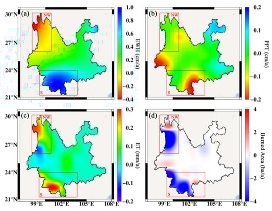
Figure 8.
The spatial distribution of long-term trend change of GRACE TWSC (a), PPT (b), ET (c) and burned area (d).
5.3.2. Seasonal Variations
Figure 9 shows the seasonal variations of TWSC, PPT, ET, relative humidity and burned area in region NW (a–d) and S (e–h) from 2003 to 2016. In the figure, PPT, ET, relative humidity and burned area data are the related change values (with the average value deducted). In Figure 9a, the monthly average TWSC in region NW is 1.61 cm, the maximum one (470.13 cm) appears in August and the minimum one (−359.99 cm) occurs in March. The monthly average burned area in region NW is approximately 0 ha, the maximum one (20,463.01 ha) occurs in January and the minimum one (−10,836.32 ha) appears in September. We found that the burned area change is positive in the months with the negative TWSC (from July to October), while the it is negative in the months with the positive TWSC (from December to March). The correlation coefficient between burned area and PPT on the seasonal scale was estimated and its value is −0.57 (see Table 3). This explains that burned area and TWSC have a strong negative correlation on the seasonal scale.
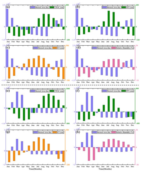
Figure 9.
The seasonal variation of burned area (ha), TWSC (cm), PPT (cm), ET (cm) and relative humidity (%) from 2003 to 2016 in the region NW (a–d) and S (e–h). The seasonal variation was obtained by subtracting the average of the corresponding months for all years from the data for each month. The four figures above the blank dotted line are for region NW, and the four ones below are for region S.
Table 3.
The correlation coefficients between burned area (BA), PPT, ET, relative humidity (RH) and TWSC on the seasonal scale in region NW.
The season with the most PPT is summer, followed by autumn and spring, and the least is winter (Figure 9b). The maximum and minimum PPT are 291.72 cm (July) and −161.51 cm (December), respectively. When the monthly PPT is negative, the monthly burned area is positive, vice versa. This suggests that there is a strong negative correlation between PPT and burned area (−0.83, see Table 3). In Figure 9c,d, the maximum ET and humidity are 262.76 cm (July) and 11.37% (August), respectively, while the minimum ones are 270.42 cm (December) and −13.72% (March), respectively. It can be seen that there are positive burned areas in the negative ET and relative humidity months (from November to March), while there are negative ones in the positive ET and relative humidity months (from April to September, ET; from June to October, relative humidity). The correlation coefficient results also support the above conclusion (burned area and ET, −0.90; burned area and humidity relatively, −0.79; Table 3).
We also compared the monthly burned area with monthly TWSC, PPT, ET and relative humidity in region S (Figure 9e–h). In this region, the maximum burned area (16,750.48 ha) appears in September, while the minimum one (−5202.83 ha) occurs in March. We can see that there are similar relationships between burned area and TWSC, PPT, ET and relative humidity. In other words, like in region NW, the positive burned areas generally occur in the months with negative TWSC, PPT, ET and relative humidity, while the negative ones appear in the months with positive TWSC, PPT, ET and relative humidity. From Table 4, the correlation coefficients between burned area and TWSC, PPT, ET and relative humidity are −0.73, −0.51, −0.35 and −0.92, respectively. However, we found that the correlation between burned area and ET is weaker than the one in region NW. Relative to region NW, the correlations between burned area and TWSC and relative humidity are stronger, while the one between burned area and PPT are weaker. The three above correlation coefficients are smaller than −0.5.
Table 4.
The correlation coefficients between burned area (BA), PPT, ET, relative humidity (RH) and TWSC on the seasonal scale in region S.
According to Figure 9, Table 3 and Table 4, we analyzed the relationship between forest fires and climate change in regions NW and S. The climate of Yunnan belongs to the Subtropical Plateau Monsoon Climate, and the dry and rainy seasons in Yunnan are relatively distinct. According to Figure 9b,f, the rainy season is from May to September and the dry season is from October to April in the two regions. From May, PPT begins to become positive and increase gradually. During the same period, ET also begins to increase as the temperature rises. The increase in PPT and ET lead to an increase in water vapor in the air, so relative humidity in the two regions rises in June (see Figure 9d,h). Similarly, TWSC also starts to increase in this month (see Figure 9a,e). The environment at this time is not conducive to the occurrence of fire. Therefore, the burned area is at a negative value during the rainy season.
The turning point appears in October. From October, PPT and ET begin to become negative. The relative humidity also becomes negative from November (NW) and January (S), and TWSC begins to become negative in December (NW) and January (S). The burned area begins to become positive in November (NW) and February (S). We found that there are significant relationships between climate change and forest fires in the two regions. Firstly, PPT and ET decrease due to climate change (from rainy season to dry season); 1–3 months later, the relative humidity and TWSC begin to fall and become negative. Immediately after, the burned area begins to increase. The correlation coefficients results (Table 3 and Table 4) show that the increase in PPT and ET causes an increase in relative humidity, and then the increase in relative humidity is reflected in TWSC. TWSC and relative humidity have a stronger negative correlation with burned area.
5.3.3. Interannual Variance
Figure 10 shows the interannual variations of TWSC, PPT, ET, relative humidity and burned area in region NW (a–d) and S (e–h) from 2003 to 2016. From these figures, the burned area has no significant correlation with TWSC, PPT, ET and relative humidity. In Figure 10a, the years with the opposite change direction in PPT and burned area are only 2003, 2006, 2008, 2009, 2014 and 2016, and there is no significant rule from the change range of the two. The same situation also appears between burned area and ET (see Figure 10b,c). From Figure 10d, it can be seen that, except for 2004 and 2010, the change direction of burned area and relative humidity are opposite. This shows that there is a significant negative correlation (−0.64, Table 5) between the two in the interannual scale. From Figure 10e, we found that the years with the opposite change direction in PPT and burned area in region S are greater than the ones in region NW, which are 2004, 2005, 2006, 2008, 2009, 2012, 2013, 2014 and 2016. This suggests that the negative correlation between TWSC and burned area in region S is stronger than that in region NW. The results of Table 5 also verify this point (−0.15 in region NW and −0.44 in region S). In Figure 10f–h, the burned area has no significant correlation with PPT, ET and relative humidity.
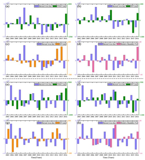
Figure 10.
The interannual variation of burned area (ha), TWSC (cm), PPT (cm), ET (cm) and relative humidity (%) from 2003 to 2016 in the region NW (a–d) and S (e–h). The interannual variation was obtained by subtracting the average of all years from the data for each year. The four figures above the blank dotted line are for region NW, and the four ones below are for region S.
Table 5.
The correlation coefficients between burned area (BA), PPT, ET, relative humidity (RH) and TWSC on the interannual scale in region NW and S.
Overall, the correlations between burned area and TWSC, PPT, ET and relative humidity in the seasonal scale are much stronger than that in the interannual scale. Except for burned area and ET in region S, the burned area has a strong correlation with TWSC, PPT, ET and relative humidity in the seasonal scale. This indicates that climate change has a strong influence on forest fires in Yunnan on a seasonal scale.
5.3.4. Climate Change before and during Extreme Forest Fire Months
To further study the relationship between climate change and forest fires in Yunnan, we compared the DMI, ENSO, PPT, ET, TWSC, water vapor column (Vcol), relative humidity (RH) and burned area in high- and low-fire years. Figure 11 shows the differences in monthly average of DMI, ENSO, PPT, ET, TWSC, Vcol, RH and burned area in high- and low-fire years.
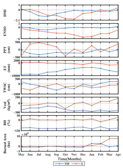
Figure 11.
Monthly evolution of Yunnan climate before and during extreme forest fire months. The differences between monthly average of PPT, ET, TWSC, Vcol, RH and burned area in high- and low-fire years (blue line: region NW, red line: region S).
From Figure 11, we found that the change trends of the above seven variances have considerable differences before and during the high-fire months. The differences between DMI and ENSO in high- and low-fire years mainly concentrate in June–October in region NW, while the ones in region S concentrate in July–January. The low PPT level appears from June to December in region NW, while it occurs from July to February in region S. The increase in ET starts in July in region NW, while the ET has no significant change in region S. Correspondingly, the water storage deficit in region NW and S appear from July to January and from September to March, respectively, which is basically the same as the time period with low PPT level. We also found that the water vapor column begins to decrease with water storage deficit. In region NW and S, the low water vapor column starts in September and lasts until February. As the water vapor column decreases, the relative humidity also decreases. The low relative humidity level in region NW and S appears from December to March and from January to March, respectively. This time period basically coincides with the high-fire months in the two regions. The maximum correlation coefficients and lag months between the different variable are shown in Table 6.
Table 6.
The maximum correlation coefficients and lag months between different variables shown in Figure 11.
Combining Figure 11 and Table 6, we plotted the figures on a series of climatic and hydrological changes before forest fires (Figure 12). In region NW, the correlation coefficients between DMI and PPT and ENSO and PPT are 0.65 and 0.84, respectively. This shows that DMI and ENSO have an important influence on PPT. When DMI is negative, as the sea temperature of East Indian Ocean increased, the water vapor transport from the Bay of Bengal weakened, resulting in a decrease in PPT in Southwest China (including Yunnan) [68]. Similarly, when the La Ninã event happened (ENSO is negative), due to the strengthening of East Asian monsoon, the PPT belt moved northward, resulting in less PPT in Southwest China [40,69]. When ENSO events and Indian Ocean Dipoles appeared together, low PPT was strengthened [70]. However, the influence of ENSO on PPT in region NW is much greater than that in region S (correlation coefficient r = 0.84 and 0.49). With low PPT and high ET, TWSC experienced an abnormal decrease, because PPT and ET are the important input and output of the regional TWSC. In region NW, PPT has a stronger correlation (0.63) with TWSC than ET (−0.30). However, the situation is opposite in region S and the correlation coefficients between PPT and ET and TWSC are 0.50 and −0.56, respectively. Four to five months later, the atmospheric water vapor and relative humidity began to decrease, which caused the climatic condition in the forest to trend to be dry, and the water content in the vegetation also decreased [71,72]. This provides powerful conditions for the occurrence and spread of forest fires. The correlation coefficients between relative humidity and atmospheric water vapor and burned area are −0.73 and −0.61 in region NW, respectively. They are −0.42 and −0.38 in region S, respectively. Before the high-fire months, GRACE TWSC has an abnormal change. This explains that TWSC has a strong connection with forest fires (correlation coefficients between TWSC and burned area are −0.70 (NW) and −0.87 (S), lag months are 5 (NW) and 6 (S)). Overall, GRACE TWSC may be useful to reflect the influence of climate change on forest fires in Yunnan.
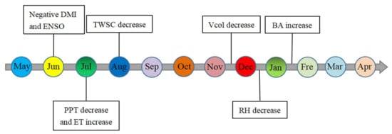
Figure 12.
A series of climatic and hydrological changes before forest fires.
To further verify the response of GRACE TWSC to climate change before forest fires, we calculated the monthly average of GRACE TWSC and PPT in region NW and S for high- and low-fire years, respectively. From Figure 13 and Figure 14, we found that there is no significant difference between PPT in high- and low-fire years in region NW and S. However, comparing Figure 13a,b, GRACE TWSC shows the different performance in region NW in high- and low-fire years, which in high-fire years is significantly lower than that in low-fire years. This situation is particularly noticeable in the southern region. GRACE TWSC is lower than −9 cm in this region in high-fire years, while it is higher than −6 cm in low-fire years, and this significant difference is more pronounced in region S. Comparing Figure 14a,b, GRACE TWSC is lower than −4 cm in most of region S in high-fire years, and higher than −3.5 cm in low-fire years. Therefore, it can be seen that GRACE TWSC reflects climate change before forest fires in the two regions better than PPT. This is because climate change affects not only PPT, but also other hydrometeorological elements, GRACE TWSC includes soil moisture, runoff, snow water, vegetation canopy water, groundwater, etc. Among them, soil moisture and vegetation canopy water are more sensitive to changes in relative humidity and water vapor in the air [35,73]. Overall, GRACE satellites can detect the influence of climate change on forest fires in Yunnan.
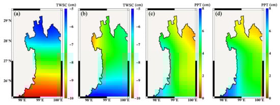
Figure 13.
The spatial distribution of GRACE TWSC and PPT for the differences between high- and low-fire years in region NW. The monthly average GRACE TWSC in high- and low-fire years (a,b) and the monthly average PPT (c,d).
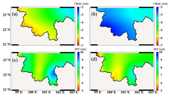
Figure 14.
The spatial distribution of GRACE TWSC and PPT for the differences between high- and low-fire years in region S. The left and right column show the monthly average of GRACE TWSC (a,b) and PPT (c,d) in high- and low-fire years, respectively.
6. Discussion
The changes of forest fires in Yunnan have significant seasonality (Figure 6), and forest fires are mainly affected by wet and dry climates [32]. In Yunnan, the dry season is from November to April of the following year, and the rainy season is from July to September [33]. The forest fires in this region are mainly concentrated in the dry season. The high-fire months in region NW and S are November–February and February–April, respectively. In the dry season, the decrease in PPT causes the ET of forest vegetation to decrease, thus atmospheric water vapor drops to a lower level (Figure 11) [73]. When the atmospheric water vapor is at a low level, the relative humidity is also relatively small (Figure 11). The lower relative humidity level creates a climatic condition more favorable for forest fires [74].
From a geographical point of view, most of the burned areas in Yunnan are mainly concentrated in region NW and S (Figure 5). By analyzing the relationship between climate change and forest fires in the two regions, we found that there is a difference in the influence of climate change on forest fires in the different regions. From Table 3 and Table 4, in region NW, the strongest correlation with burned area is ET (−0.90), followed by PPT (−0.83), relative humidity (−0.79) and GRACE TWSC (−0.57). However, in region S, according to the order of correlation with burned area, the order is relative humidity (−0.92), GRACE TWSC (−0.73), PPT (−0.51) and ET (−0.35). The reason for the above difference between the two regions may be the regional climate types. Region NW belongs to semi-dry and semi-wet climate, and region S belongs to a wet climate [74]. The biggest feature of semi-dry and semi-wet climate is that ET is relatively stronger with less PPT. The huge ET and lower PPT levels cause the water storage of local vegetation to be lower [15,16], resulting in a higher number of combustibles, which in turn increases the possibility of forest fires [25,32]. The wet climate is mainly characterized by humid air and abundant PPT, and the vegetation in region S is dominated by tropical rainforests. Therefore, relative humidity in the air is the main factor affecting forest fires [35]. ET is an important output item of TWSC, while relative humidity has an important influence on vegetation canopy water and soil moisture [71].
Our study found that less GRACE TWSC appeared before forest fires in Yunnan, which is related to climate change. Therefore, GRACE TWSC data may be used to predict the risk of forest fires [35]. From Figure 13 and Figure 14, GRACE TWSC can better reflect local climate change before forest fires than PPT. It can provide a new way of thinking and methods for forest fire prevention.
7. Conclusions
To detect the influence of climate change on forest fires in Yunnan, we used GCTH and least square method to fused TWSC results from six GRACE solutions to improve the accuracy and reliability of TWSC results, and analyzed the relationship between climate factors, GRACE TWSC and burned area. The results show that the temporal distribution of burned area has a significant seasonality, and climate factors and GRACE TWSC have a strong correlation with burned area on the seasonal scale. GRACE TWSC changed significantly in the first few months of forest fires, and it can reflect local climate change. Therefore, GRACE TWSC can well reflect local climate change before forest fires occur.
Our research results will provide a new research method for the influence of climate change on forest fires in Yunnan, and provide strong data support for local governments to formulate forest fire prevention measures.
Author Contributions
Conceptualization, L.C. and X.W.; methodology, L.C.; software, C.L.; validation, C.Y. and Q.L.; data curation, C.L. and L.C.; writing—original draft preparation, C.L.; writing—review and editing, C.Y., Q.L. and X.W.; supervision, Z.Z and G.W.; funding acquisition, Z.Z. and G.W. All authors have read and agreed to the published version of the manuscript.
Funding
This research was funded by the Open Fund of Wuhan, Gravitation and Solid Earth Tides, National Observation and Research Station (Grant No. WHYWZ202102), the National Natural Science Foundation of China (Grant No. 42074172, 41931074 & 42004013), Scientific Research Fund from Institute of Seismology, CEA and National Institute of Natural Hazards, Ministry of Emergency Management of China (Grant No. IS201956307), Science for Earthquake Resilience (Grant No. XH21021), Foundation of Young Creative Talents in Higher Education of Guangdong Province (Grant No. 2019KQNCX009) and Guangzhou Science and Technology Project (Grant No. 202102020526).
Institutional Review Board Statement
Not applicable.
Informed Consent Statement
Not applicable.
Data Availability Statement
GRACE RL06 data from CSR, GFZ, JPL and ITSG: http://icgem.gfz-potsdam.de/series (accessed on 6 December 2021); In-situ precipitation data: http://data.cma.cn (accessed on 6 December 2021); Burned area data: https://www.geo.vu.nl/~gwerf/GFED/GFED4/ (accessed on 6 December 2021); ET gridded data: sftp://hydras.ugent.be (accessed on 6 December 2021); Relative humidity data: http://www.esrl.noaa.gov/psd/data/gridded/data.ncep.reanalysis2.html (accessed on 6 December 2021); monthly atmospheric column water vapor gridded data: http://disc.sci.gsfc.nasa.gov/AIRS/data-holdings/by-data-product/airsL3_STM.shtml (accessed on 6 December 2021); Extreme climate index data: https://psl.noaa.gov/ (accessed on 6 December 2021).
Acknowledgments
We are grateful to CSR, GFZ, JPL and ITSG for providing the monthly GRACE gravity field solutions, and to the Goddard Space Flight Center for providing the monthly GLDAS-2.1 data, to the China National Meteorological Science Data Center for providing the monthly precipitation products, to the Global Fire Emission Database Version 4.1s for providing burned area data, to the Global Land Evaporation Amsterdam Model for providing ET data, to the Physical Sciences Laboratory at the National Oceanic and Atmospheric Administration for providing relative humidity data, to the National Centers for Environmental Prediction Reanalysis project for providing atmospheric column water vapor data, to the National Oceanic and Atmospheric Administration for providing extreme climate index data, and to MathWorks for providing Matlab for all data processing in our study.
Conflicts of Interest
The authors declare no conflict of interest.
References
- Guo, T.N. Fire situation in 2004 and tendency as well as counter measures in the future. Fire Sci. Technol. 2005, 24, 263–266. (In Chinese) [Google Scholar]
- Girardin, M.P.; Ali, A.A.; Carcaill, C.; Gauthier, S.; Hely, C.; Le Goff, H.; Terrire, A.; Bergeron, Y. Fire in managed forest of eastern Canada: Risks and option. For. Ecol. Manag. 2013, 294, 238–249. [Google Scholar] [CrossRef]
- Sliva, C.A.; Santill, G.; Sano, E.E.; Laneve, G. Fire occurrences and greenhouse gas emissions from deforestation in the Brazilian Amazon. Remote Sens. 2021, 13, 376. [Google Scholar] [CrossRef]
- Ehsani, M.R.; Arevalo, J.; Risanto, C.B.; Javadian, M.; Denine, C.J.; Arabzadeh, A.; Venegas-Quiñones, H.L.; Dell’Oro, A.P.; Behrangi, A. 2019-2020 Australia Fire and its relationship to hydroclimatological and vergetation variabilities. Water 2020, 12, 3067. [Google Scholar] [CrossRef]
- Balling, R.C.; Meyer, G.A.; Wells, S.G. Relation of surface climate and burned area in Yellowstone National Park. Agric. For. Meteoro. 1992, 60, 285–293. [Google Scholar] [CrossRef]
- Vélez, R. High intensity forest fires in the Mediterranean basin: Natural and socioeconomic causes. Disaster Manag. 1993, 5, 16–20. [Google Scholar]
- Mouillot, F.; Rambal, S.; Joffre, R. Simulating climate change impacts on fire frequency and vegetation dynamics in a Mediterranean-type ecosystem. Glob. Chang.Biol. 2002, 8, 423–437. [Google Scholar] [CrossRef]
- Fried, J.S.; Gilless, J.K.; Riley, W.J.; Moody, T.J.; de Blas, C.S.; Hayhoe, K.; Moritz, M.; Stephens, S.; Torn, M. Predicting the effect of climate change on wildfire behavior and initial attack success. Clim. Chang. 2008, 87, 251–264. [Google Scholar] [CrossRef] [Green Version]
- Zhong, S.Y.; Wang, T.; Sciusco, P.; Shen, M.C.; Pei, L.S.; Nikolic, J.; Mckeehan, K.; Kashogwe, H.; Hatami-Beiglou, P.; Camacho, K.; et al. Will land use cover change drive atmospheric conditions to become more conducive to wildfire in the United States? Int. J. Climatol. 2021, 41, 3578–3597. [Google Scholar] [CrossRef]
- Flannigan, M.D.; Stocks, B.J.; Wotton, B.M. Climate change and forest fires. Sci. Total Environ. 2000, 262, 221–229. [Google Scholar] [CrossRef]
- Fried, J.S.; Torn, M.S.; Mills, E. The impact of climate change on wildfire severity: A regional forecast for northern California. Clim. Chang. 2004, 64, 169–191. [Google Scholar] [CrossRef]
- Shu, L.F.; Tian, X.R.; Kou, X.J. The focus and progress on forest fire research. World For. Res. 2003, 16, 37–40. (In Chinese) [Google Scholar]
- Zhao, F.J.; Shu, L.F.; Di, X.Y.; Tian, X.R.; Wang, M.Y. Changes in the occurring data of forest fires in the Inner Mongolia Daxing anling forest region under global warming. Sci. Silvae Sin. 2009, 45, 166–172. (In Chinese) [Google Scholar]
- Roads, J.; Fujioka, F.; Chen, S.; Burgan, R. Seasonal fire danger forecasts for the USA. Int. J. Wildland Fire 2005, 14, 1–18. [Google Scholar] [CrossRef]
- Collins, M.; Omi, P.N.; Chapman, P.L. Regional relationships between climate and wildfire burned area in the Interior West. Canadian J. For. Res. 2006, 36, 699–709. [Google Scholar] [CrossRef]
- Preisler, K.; Westerling, A.L. Statistical model for forecasting monthly large forest fire events in western United States. J. Appl. Meteorol.Climatol. 2007, 46, 1020–1030. [Google Scholar] [CrossRef] [Green Version]
- Badia, A.; Sauri, D.; Cerdan, R.; Llurdés, J.C. Causality and management of forest fires in Mediterranean environments: An example from Catalonia. Environ. Hazards 2002, 4, 23–32. [Google Scholar]
- Soja, J.; Tehebakova, N.M.; French, N.H.F.; Flannigan, M.D.; Shugart, H.H.; Stocks, B.J.; Sukhinin, A.I.; Parfenova, E.I.; Chapin, F.S., III; Stackhouse, P.W., Jr. Climate-induced boreal forest change: Predictions versus current observations. Glob. Planet. Chang. 2007, 56, 274–296. [Google Scholar] [CrossRef] [Green Version]
- Jentsch, A.; Beierkuhnlein, C. Research frontiers in climate change: Effects of extreme meteorological events on ecosystems. Comptes Rendus Geosci. 2008, 340, 621–628. [Google Scholar] [CrossRef]
- Swetnam, T.W.; Betancourt, J.L. Fire-southern oscillation relations in the southwestern United States. Science 1990, 249, 1017–1020. [Google Scholar] [CrossRef]
- Jones, C.S.; Shriver, J.F.; O’Brien, J.J. The effects of El Niño on rainfall and fire in Florida. Florida Geogr. 1999, 30, 55–69. [Google Scholar]
- Swetnam, T.W.; Betancourt, J.L. Mesoscale disturbance and ecological response to decadal climate variability in the American Southwest. J. Clim. 1998, 11, 3128–3147. [Google Scholar] [CrossRef]
- Chen, J.; Randerson, T.; Morton, D.C. Forecasting fire season severity in South America using sea surface temperature anomalies. Science 2011, 334, 787–791. [Google Scholar] [CrossRef] [Green Version]
- Gillett, P.; Weaver, A.J.; Zwiers, F.W.; Flannigan, M.D. Detecting the effect of climate change on Canadian forest fires. Geophys. Res. Lett. 2004, 31, L18211. [Google Scholar] [CrossRef] [Green Version]
- Heyerdahl, E.K.; McKenzie, D.; Daniels, L.D.; Hessl, A.E.; Littell, J.S.; Mantua, N.J. Climate drives of regionally synchronous fires in the inland Northwest (1651–1900). Int. J. Wildland Fire 2008, 17, 40–49. [Google Scholar] [CrossRef] [Green Version]
- Westerling, L.; Gershunov, A.; Brown, T.J.; Cayan, D.R.; Dettinger, M.D. Climate and wildfire in the western United States. Bull. Amer. Meteorol. Soc. 2003, 84, 595–604. [Google Scholar] [CrossRef] [Green Version]
- Pausas, J.G. Changes in fire and climate in the Eastern Iberian Peninsula. Clim. Chang. 2004, 63, 337–350. [Google Scholar] [CrossRef]
- Tapley, B.D.; Bettadpur, S.; Ries, J.C.; Thompson, P.F.; Watkins, M.M. GRACE measurements of mass variability in the Earth system. Science 2004, 305, 503–505. [Google Scholar] [CrossRef] [Green Version]
- Wahr, J.; Melenaar, M.; Bryan, F. Time variability of the Earth’s gravity field: Hydrological and oceanic effects and their possible detection using GRACE. J. Geophys. Res: Solid Earth 1998, 103, 30205–30229. [Google Scholar] [CrossRef]
- Xie, J.K.; Xu, Y.P.; Wang, Y.T.; Gu, H.T.; Wang, F.M.; Pan, S.L. Influence of climatic variability and human activities on terrestrial water storage variations across the Yellow River basin in the recent decade. J. Hydr. 2019, 579, 124218. [Google Scholar] [CrossRef]
- Cui, L.L.; Zhang, C.; Luo, Z.C.; Wang, X.L.; Li, Q.; Liu, L.L. Using the local drought data and GRACE/GRACE-FO data to characterize the drought events in Mainland China from 2002 to 2020. Appl. Sci. 2021, 11, 9594. [Google Scholar] [CrossRef]
- Chen, F. The Response of Forest Fire to Climate Change and Fire Trend Prediction in Yunnan Province. Ph.D. Thesis, Beijing Forestry University, Beijing, China, 24 June 2015. (In Chinese). [Google Scholar]
- Chen, F.; Fan, Z.F.; Niu, S.K.; Zheng, J.M. The influence of precipitation and consecutive dry days on burned areas in Yunnan province, southwestern China. Adv. Meteorol. 2014, 2014, 748923. [Google Scholar] [CrossRef] [Green Version]
- Chen, Y.; Velicogna, I.; Famiglietti, J.S.; Randerson, T. Satellite observation of terrestrial water storage provide early warning information about drought and fire season severity in the Amazon. J. Geophys. Res. 2013, 118, 495–504. [Google Scholar] [CrossRef] [Green Version]
- Han, J.C.; Tangdamrongsub, N.; Hwang, C.; Abidin, H.Z. Intensified water storage loss by biomass burning in Kalimantan: Detection by GRACE. J. Geophys. Res. 2017, 112, 2409–2430. [Google Scholar] [CrossRef]
- Zhang, B.; Liu, L.; Yao, Y.; van Dam, T.; Khan, S.A. Improving the estimate of the secular variation of Greenland ice mass in the recent decades by incorporating a stochastic process. Earth Planet Sci. Lett. 2020, 549, 116518. [Google Scholar] [CrossRef]
- Yang, M. General situation of forest resources distribution in Yunnan province. Yunnan For. Investig. Plan. Des. 1995, 4, 12–14. (In Chinese) [Google Scholar]
- Cheng, M.; Tapley, B.D. Variations in the Earth’s oblateness during the past 28 years. J. Geophys. Res. 2004, 109, B09402. [Google Scholar] [CrossRef]
- Swenson, S.; Chambers, D.; Whar, J. Estimating geocenter variations form a combination of GRACE and ocean model output. J. Geophys. Res. Solid Earth. 2008, 113, 194–205. [Google Scholar] [CrossRef] [Green Version]
- Cui, L.L.; Zhang, C.; Yao, C.L.; Luo, Z.C.; Wang, X.L.; Li, Q. Analysis of the influencing factors of drought events based on GRACE data under different climatic conditions: A case study in Mainland China. Water 2021, 13, 2575. [Google Scholar] [CrossRef]
- Cui, L.L.; Song, Z.; Luo, Z.C.; Zhong, B.; Wang, X.L.; Zou, Z.B. Comparison of terrestrial water storage changes derived from GRACE/GRACE-FO and Swarm: A case study in the Amazon River Basin. Water 2020, 12, 3128. [Google Scholar] [CrossRef]
- Wiese, D.N.; Yuan, D.N.; Boening, C.; Landerer, E.W.; Watkins, M.M. JPL Grace Mascon Ocean, Ice and Hydrology Equivalent Water Height Release 06 Coastal Resolution Improvement (CRI) Filter Version 1.0; DAAC: Pasadena, CA, USA, 2018. [Google Scholar]
- Save, H.; Bettadpur, S.; Tapley, B.D. High resolution CSR GRACE RL05 Mascons. J. Geophys. Res. Solid Earth 2016, 121, 7547–7569. [Google Scholar] [CrossRef]
- Yan, X.; Zhang, B.; Yao, Y.B.; Yang, Y.J.; Li, J.Y.; Ran, Q.S. GRACE and land surface models reveal severe drought in eastern China in 2019. J. Hydr. 2021, 601, 126640. [Google Scholar] [CrossRef]
- Sun, Y.; Riva, R.; Ditmar, P. Optimzing estimates of annual variations and trends in geocenter motion and J2 from a combination of GRACE data and geophysical models. J. Geophys. Res. Solid Earth 2016, 121, 8352–8370. [Google Scholar] [CrossRef] [Green Version]
- Richard, P.W.; Argus, D.F. Drummond, R. comment on “an assessment of the ICE-6G-_C (VM5a) glacial isostatic adjustment model” by Purcell et al. J. Geophys. Res. Solid Earth 2018, 123, 2019–2028. [Google Scholar] [CrossRef]
- Giglio, L.; Randerson, J.T.; van der Werf, G.R. Analysis of daily, monthly, and annual burned area using the fourth-generation global fire emission database (GFED4). J. Geophys. Res. Biogeosci. 2013, 118, 317–328. [Google Scholar] [CrossRef] [Green Version]
- Van der Werf, G.R.; Randerson, J.T.; Giglio, L.; Collatz, G.J.; Mu, M.; Kasibhatla, P.S.; Morton, D.C.; Defries, R.S.; Jin, Y.; van Leeuwen, T.T. Global fire emission and the contribution of deforestation, savanna, forest, agricultural, and peat fires (1997–2009). Atmos. Chem. Phys. 2010, 10, 11707–11735. [Google Scholar] [CrossRef] [Green Version]
- Giglio, L.; Randerson, J.T.; Van der Werf, G.R.; Kasibhatla, P.S.; Collatz, G.J.; Morton, D.C.; DeFries, R.S. Assessing variability and long-term trends in burned area by merging multiple satellite fire products. Biogeoences 2010, 7, 1171–1186. [Google Scholar] [CrossRef] [Green Version]
- Miralles, D.G.; Holmes, T.R.H.; de Jeu, R.A.M.; Gash, H.; Meesters, A.G.C.A.; Dolman, A.J. Global land surface evaporation estimated from satellite-based observations. Hydrol. Earth Syst. Sci. 2011, 15, 453–469. [Google Scholar] [CrossRef] [Green Version]
- Martens, B.D.G.; Miralles, H.; Lievens, H.; van der Schalie, R.; de Jeu, R.A.M.; Férnandez-Prieto, D.; Beck, H.E.; Dorigo, W.A.; Verhoest, N.E.C. GLEAM v3: Satellite-based land evaporation and root-zone soil moisture. Geosci. Model Dev. 2017, 10, 1903–1925. [Google Scholar] [CrossRef] [Green Version]
- Kanamitsu, M.; Ebisuzaki, W.; Woollen, J.; Hnilo, J.J.; Fiorino, M.; Potter, G.L. NCEP-DOE AMIP-II Reanalysis (R-2). Bull. Amer. Meteorol. Soc. 2002, 83, 1631–1643. [Google Scholar] [CrossRef]
- Chahine, M.T.; Pagano, T.S.; Aumann, H.H.; Atlas, R.; Barnet, C.; Blaisdell, J.; Chen, L.; Divakarla, M.; Fetzer, E.J.; Goldberg, M.; et al. AIRS: Improving weather forecasting and providing new data on greenhouse gases. Bull. Biol. Sci. 2006, 87, 911–926. [Google Scholar] [CrossRef] [Green Version]
- Zheng, C.Y.; Huang, F.; Pu, G.M. The interannual and decadal variability of precipitation for Yunnan province in rainy season and its relationship with tropical upper layer heat content. J. Trop. Meteorol. 2003, 19, 299–307. (In Chinese) [Google Scholar]
- Saji, N.; Goswami, B.N.; Vinayachandran, P.; Yamagata, T. A dipole model in the tropical Indian Ocean. Nature 1999, 401, 360–363. [Google Scholar] [CrossRef] [PubMed]
- Long, D.; Pan, Y.; Zhou, J.; Chen, Y.; Hou, X.; Hong, Y.; Scanlon, B.R.; Longuevergne, L. Global analysis of spatiotemporal variability in merged total water storage changes using multiple GRACE products and global hydrological models. Remote Sens. Environ. 2017, 192, 198–216. [Google Scholar] [CrossRef]
- Yao, C.L.; Li, Q.; Luo, Z.C.; Wang, C.R.; Zhang, R.; Zhou, B.Y. Uncertainties in GRACE-derived terrestrial water storage changes over mainland China based on a generalized three cornered hat method. Chines J. Geophys. 2019, 62, 883–897. (In Chinese) [Google Scholar]
- Tavella, P.; Premoli, A. Estimating the instabilities of N clock by measuring differences of their readings. Metrologia 1994, 30, 479–486. [Google Scholar] [CrossRef]
- Koot, L.; de Viron, O.; Dehant, V. Atmospheric angular momentum time-series: Characterization of their internal noise and creation of a combined series. J. Geod. 2006, 79, 663–674. [Google Scholar] [CrossRef]
- Galindo, F.J.; Palacio, J. Post-processing ROA data clocks for optimal stability in the ensemble timescale. Metrologia 2003, 40, S236–S244. [Google Scholar] [CrossRef]
- Galindo, F.J.; Palacio, J. Estimating the instabilities of N correlated clocks. In Proceedings of the 31st Annual Precise Time and -Time Interval (PTTI) Meeting, Real Instituto y Observatorio de la Armada, Dana Point, CA, USA, 7–9 December 1999; pp. 285–296. [Google Scholar]
- Premoli, A.; Tavella, P. A revisited three-cornered hat method for estimating frequency standard instability. IEEE Trans. Instrum. Meas. 1993, 42, 7–13. [Google Scholar] [CrossRef]
- Xu, Y.F.; Lin, Z.H.; Wu, C.L. Spatiotemporal variation of the burned area and its relationship with climatic factors in Central Kazakhtan. Remote Sens. 2021, 13, 313. [Google Scholar] [CrossRef]
- Zhang, Z.; Chao, B.; Chen, J.L.; Wilson, C. Terrestrial water storage anomalies of Yangtze River basin droughts observed by GRACE and Connections with ENSO. Glob. Planet Chang. 2015, 126, 35–45. [Google Scholar] [CrossRef]
- Zou, Z.B.; Zhang, C.; Cui, L.L.; Zhong, B.; Gao, S. The long-term change of terrestrial water storage in mainland China detected by gravity satellite in the past 16 years. Sic. Technol. Eng. 2021, 21, 1701–1706. (In Chinese) [Google Scholar]
- Guo, L. Study on Forest Fire Suppression Methods of Alpine Forests in Yunnan Province. Master’s Thesis, Chinese Academy of Forestry, Beijing, China, 20 June 2015. (In Chinese). [Google Scholar]
- Li, M.H. Design of fireproof belt in Yunnan forest nature center. For. Fire Prev. 2002, 1, 28–30. (In Chinese) [Google Scholar]
- Huang, T.C.; Hua, W. Relationship between the South Indian Ocean Dipole and the September precipitation in Southwest China. Plateau Mt. Meteorol. Res. 2020, 40, 41–47. (In Chinese) [Google Scholar]
- Liu, Y.Q.; Ding, Y.H. Influence of ENSO events on weather and climate of China. J. Appl. Meteorol. Sci. 1992, 3, 473–481. [Google Scholar]
- Shi, Y. Climate Change Characteristics and Main Causes of Precipitation in Yunnan. Master’s Thesis, Yunnan University, Kunming, China, 11 June 2018. (In Chinese). [Google Scholar]
- Asner, G.P.; Alencar, A. Drought impact on the Amazon forest: The remote sensing perspective. New Phytol. 2010, 187, 569–578. [Google Scholar] [CrossRef] [PubMed]
- Tosca, M.G.; Randerson, J.T.; Zender, C.S.; Flanner, M.G.; Rasch, P.J. Do biomass burning aerosols intensify drought in equatorial Asia during El Niño? Atmos. Chem. Phys. 2010, 10, 3515–3528. [Google Scholar] [CrossRef] [Green Version]
- Jipp, P.H.; Nepstad, D.C.; Cassel, D.K.; de Carvallo, C.R. Deep soil moisture storage and transpiration in forest and pastures of seasonally-dry Amazonia. Clim. Chang. 1998, 39, 395–412. [Google Scholar] [CrossRef]
- Chen, F.; Niu, S.K.; Tong, X.J.; Zhao, J.L.; Sun, Y.; He, T.F. The impact of precipitation regimes on forest fires in Yunnan Province, Southwest China. Sci. World J. 2014, 2014, 326782. [Google Scholar] [CrossRef] [Green Version]
Publisher’s Note: MDPI stays neutral with regard to jurisdictional claims in published maps and institutional affiliations. |
© 2022 by the authors. Licensee MDPI, Basel, Switzerland. This article is an open access article distributed under the terms and conditions of the Creative Commons Attribution (CC BY) license (https://creativecommons.org/licenses/by/4.0/).