
Spectral-Based Monitoring of Climate Effects on the Inter-Annual Variability of Different Plant Functional Types in Mediterranean Cork Oak Woodlands


Abstract
:1. Introduction
2. Materials and Methods
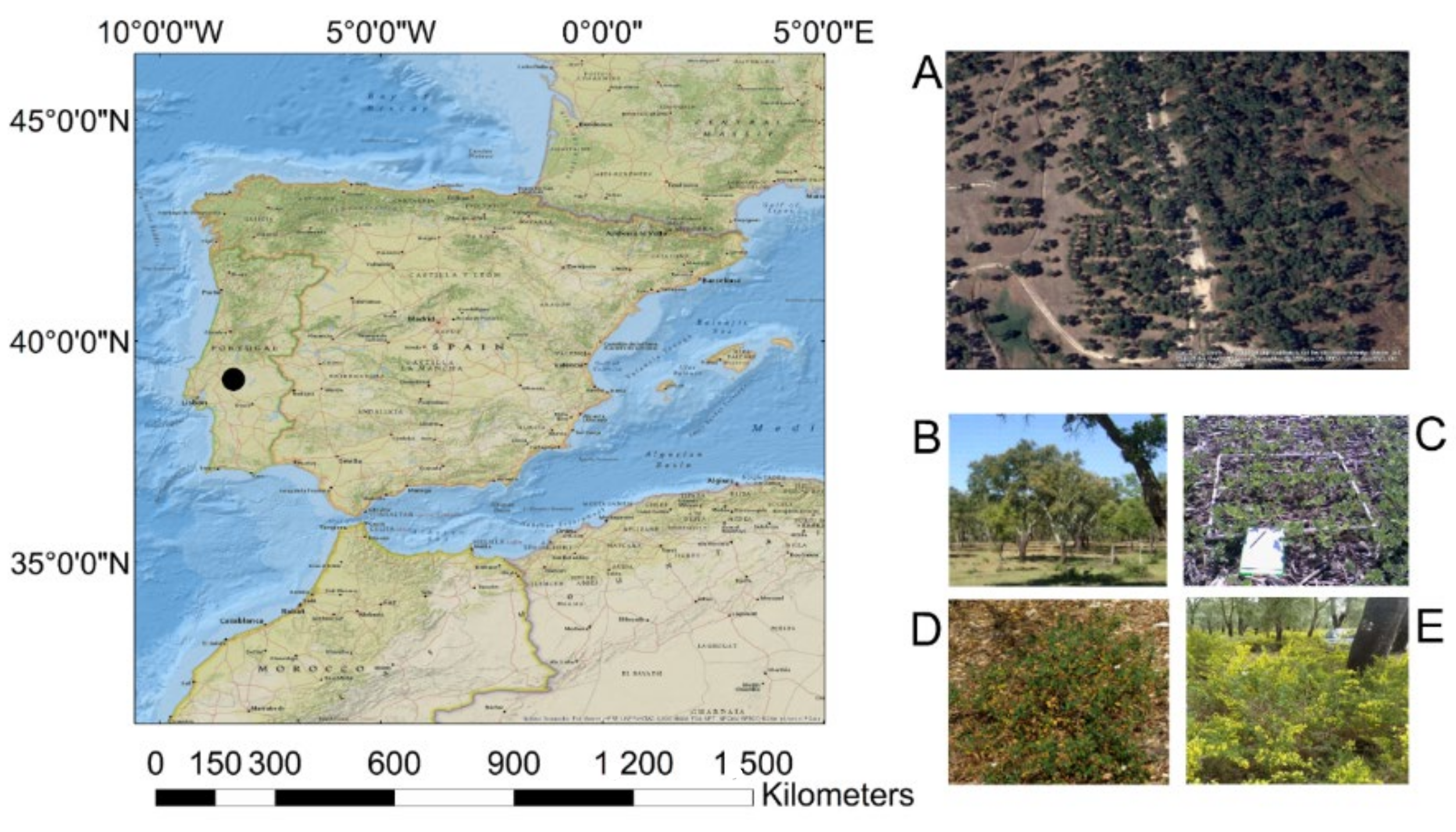
2.1. Study Area
2.2. Data Collection
2.2.1. Spectral Data
2.2.2. Climate Data
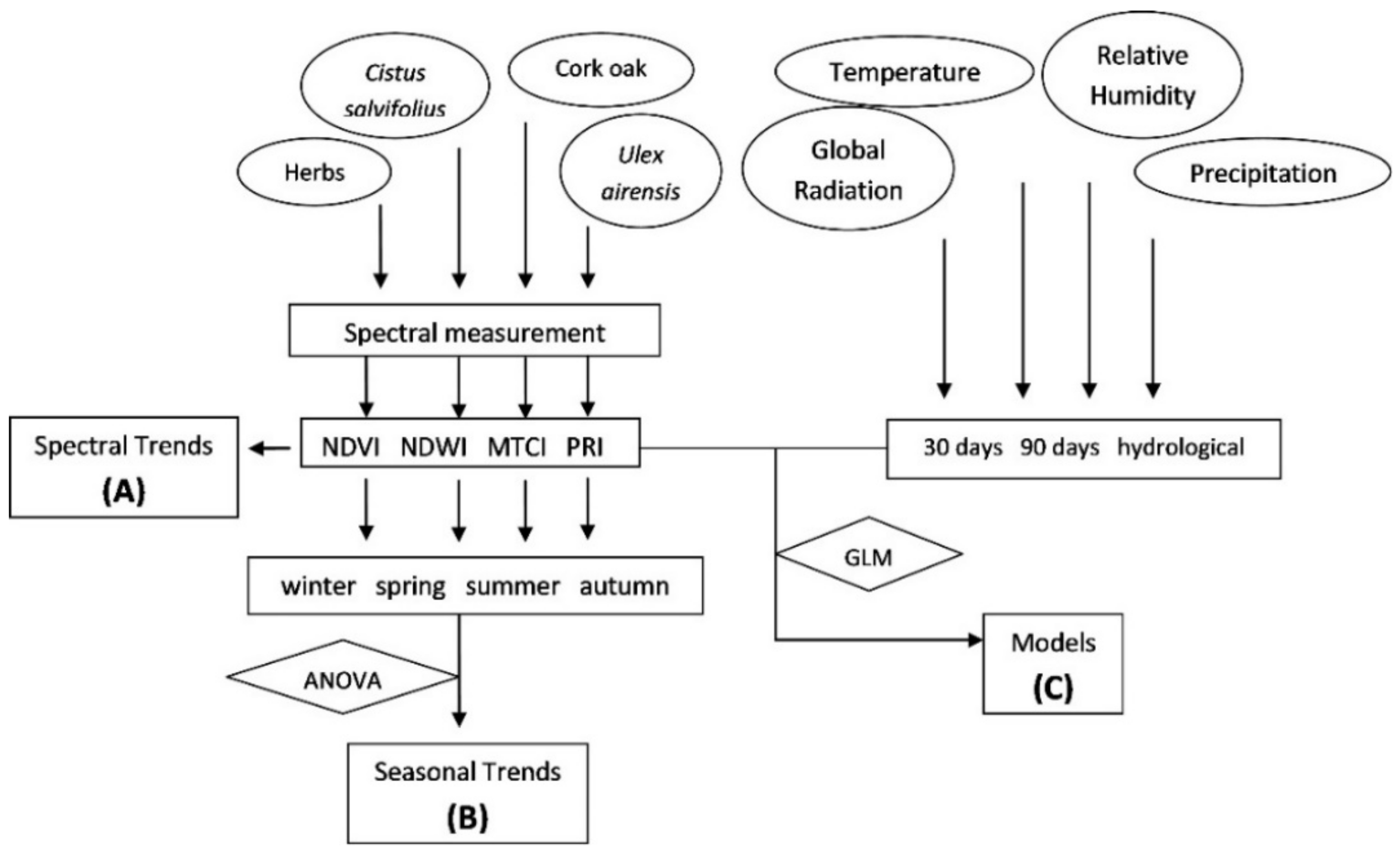
2.3. Data Analysis
3. Results
3.1. Climatic Time Series
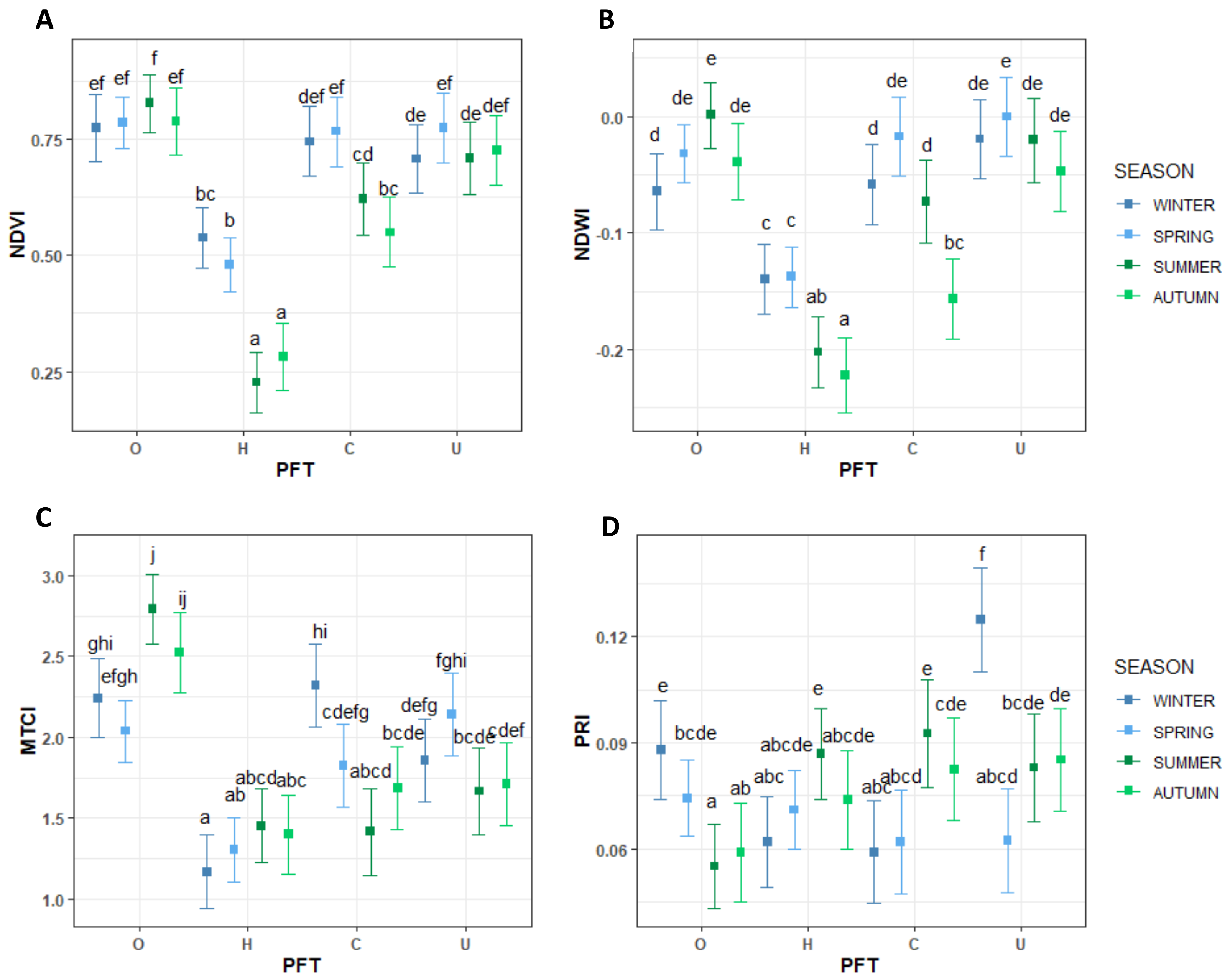
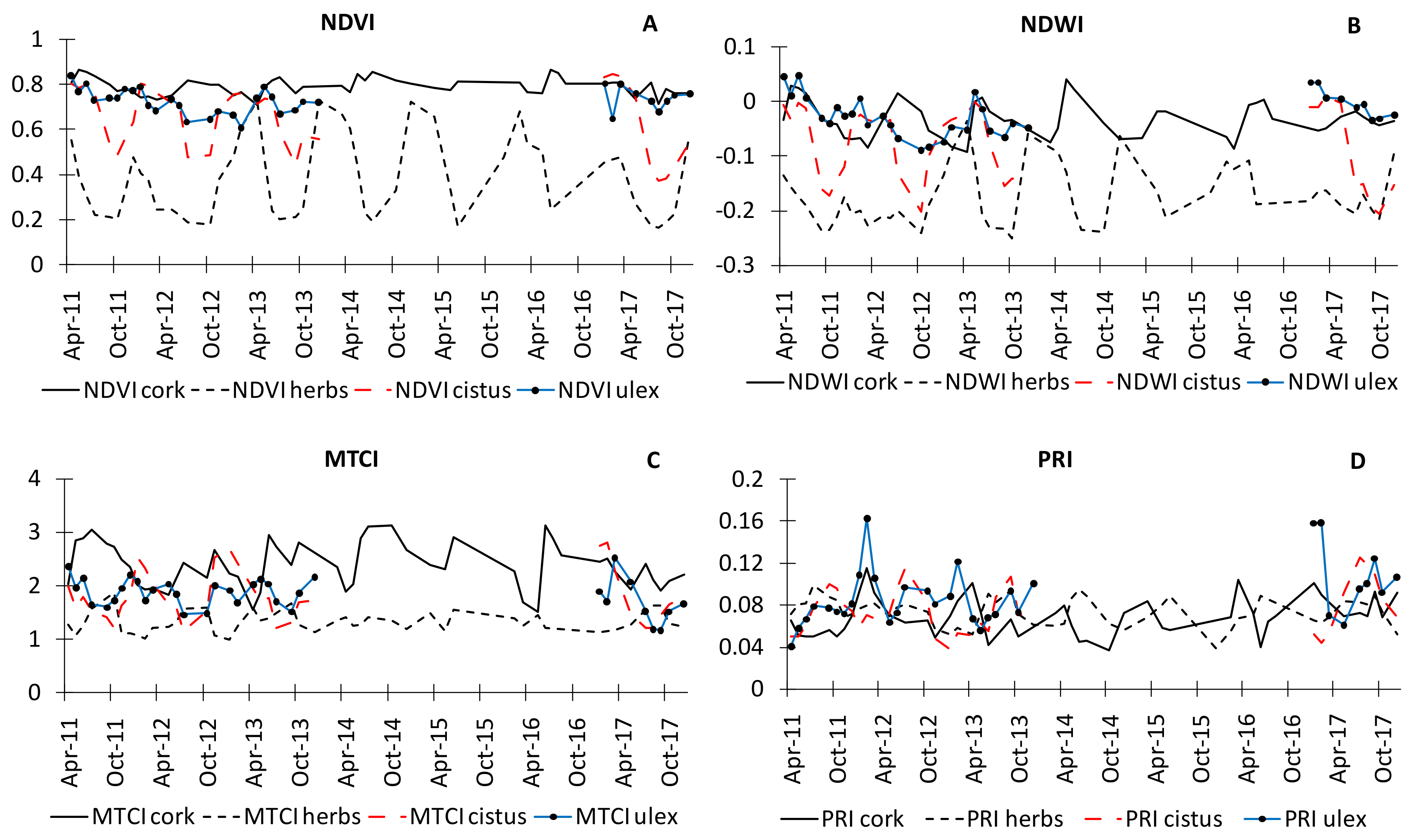
3.2. Temporal Trends of Vegetation Indices
3.3. The Influence of Climate
4. Discussion
4.1. Climate Influence
4.1.1. Cork Oak
4.1.2. Herbaceous Vegetation
4.1.3. Shrubs
4.2. Vegetation Indices Temporal Trends
4.2.1. Cork Oak
4.2.2. Herbaceous Vegetation
4.2.3. Shrubs
5. Conclusions
Author Contributions
Funding
Institutional Review Board Statement
Informed Consent Statement
Data Availability Statement
Acknowledgments
Conflicts of Interest
References
- Joffre, R.; Rambal, S.; Damesin, C. Funtional attributes in Mediterranean-type ecosystem. In Handbook of Funtional Plant Ecology; Marcel Dekker: New York, NY, USA, 1999; pp. 347–380. [Google Scholar]
- Bugalho, M.N.; Caldeira, M.C.; Pereira, J.S.; Aronson, J.; Pausas, J.G. Mediterranean cork oak savannas require human use to sustain biodiversity and ecosystem services. Front. Ecol. Environ. 2011, 9, 278–286. [Google Scholar] [CrossRef] [Green Version]
- ICNF IFN6. Principais Resultados—Relatório Sumário v1.0; Instituto da Conservação da Natureza e das Florestas, I.P.: Lisboa, Portugal, 2019.
- Costa, A.; Pereira, H.; Madeira, M. Analysis of spatial patterns of oak decline in cork oak woodlands in Mediterranean conditions. Ann. For. Sci. 2010, 67, 204. [Google Scholar] [CrossRef]
- Peñuelas, J.; Sardans, J.; Filella, I.; Estiarte, M.; Llusià, J.; Ogaya, R.; Carnicer, J.; Bartrons, M.; Rivas-Ubach, A.; Grau, O.; et al. Impacts of global change on Mediterranean forests and their services. Forests 2017, 8, 463. [Google Scholar] [CrossRef] [Green Version]
- Zalloni, E.; Battipaglia, G.; Cherubini, P.; Saurer, M.; De Micco, V. Wood growth in pure and mixed Quercus ilex l. Forests: Drought influence depends on site conditions. Front. Plant Sci. 2019, 10, 397. [Google Scholar] [CrossRef]
- Collins, M.; Knutti, R.; Arblaster, J.; Dufresne, J.-L. Long-term climate change: Projections, commitments and irreversibility. In Climate Change 2013 the Physical Science Basis: Working Group I Contribution to the Fifth Assessment Report of the Intergovernmental Panel on Climate Change; Stocker, T.F., Qin, D., Plattner, G.-K., Tignor, M., Allen, S.K., Boschung, J., Nauels, A., Xia, Y., Bex, V., Midgley, P.M., Eds.; Cambridge University Press: Cambridge, UK; New York, NY, USA, 2013; pp. 1029–1136. ISBN 978-1-107-415324. [Google Scholar]
- Díaz Barradas, M.C.; Zunzunegui, M.; Tirado, R.; Ain-Lhout, F.; García Novo, F. Plant functional types and ecosystem function in Mediterranean shrubland. J. Veg. Sci. 1999, 10, 709–716. [Google Scholar] [CrossRef] [Green Version]
- Duckworth, J.C.; Kent, M.; Ramsay, P.M. Plant functional types: An alternative to taxonomic plant community description in biogeography? Prog. Phys. Geogr. Earth Environ. 2000, 24, 515–542. [Google Scholar] [CrossRef]
- Costa, A.; Barbosa, I.; Roussado, C.; Graça, J.; Spiecker, H. Climate response of cork growth in the Mediterranean oak (Quercus suber L.) woodlands of southwestern Portugal. Dendrochronologia 2016, 38, 72–81. [Google Scholar] [CrossRef]
- Cerasoli, S.; Costa e Silva, F.; Silva, J.M.N. Temporal dynamics of spectral bioindicators evidence biological and ecological differences among functional types in a cork oak open woodland. Int. J. Biometeorol. 2015, 60, 813–825. [Google Scholar] [CrossRef]
- Correia, A.C.; Costa-e-Silva, F.; Dubbert, M.; Piayda, A.; Pereira, J.S. Severe dry winter affects plant phenology and carbon balance of a cork oak woodland understorey. Acta Oecol. 2016, 76, 1–12. [Google Scholar] [CrossRef]
- Aranda, I.; Castro, L.; Alía, R.; Pardos, J.A.; Gil, L. Low temperature during winter elicits differential responses among populations of the Mediterranean evergreen cork oak (Quercus suber). Tree Physiol. 2005, 25, 1085–1090. [Google Scholar] [CrossRef] [Green Version]
- Grant, O.M.; Tronina, Ł.; García-Plazaola, J.I.; Esteban, R.; Pereira, J.S.; Manuela Chaves, M. Resilience of a semi-deciduous shrub, Cistus salvifolius, to severe summer drought and heat stress. Funct. Plant Biol. 2015, 42, 219–228. [Google Scholar] [CrossRef] [PubMed]
- Wang, P.; Huang, K.; Hu, S. Distinct fine-root responses to precipitation changes in herbaceous and woody plants: A meta-analysis. New Phytol. 2020, 225, 1491–1499. [Google Scholar] [CrossRef] [PubMed]
- Atherton, B.C.; Morgan, M.T.; Shearer, S.A.; Stombaugh, T.S.; Ward, A.D. Site-specific farming: A perspective on information needs, benefits and limitations. J. Soil Water Cons. 1999, 54, 455–461. [Google Scholar]
- Xue, J.; Su, B. Significant remote sensing vegetation indices: A review of developments and applications. J. Sens. 2017, 2017, 17. [Google Scholar] [CrossRef] [Green Version]
- Al-Ali, Z.M.; Abdullah, M.M.; Asadalla, N.B.; Gholoum, M. A comparative study of remote sensing classification methods for monitoring and assessing desert vegetation using a UAV-based multispectral sensor. Environ. Monit. Assess. 2020, 192, 389. [Google Scholar] [CrossRef] [PubMed]
- Govender, M.; Chetty, K.; Bulcock, H. A review of hyperspectral remote sensing and its application in vegetation and water resource studies. Int. Water Irrig. 2007, 27, 20–24. [Google Scholar] [CrossRef] [Green Version]
- Rouse, W.; Haas, H.; Deering, W. Monitoring vegetation systems in the reat plains with ERTS. In Third Earth Resources Technology Satellite-1 Symposium: The Proceedings of a Symposium Held by Goddard Space Flight Center, Washington, DC, USA, 10–14 December 1973; Scientific and Technical Information Office, National Aeronautics and Space Administration (NASA): Hampton, VA, USA, 1974. [Google Scholar]
- Godinho, S.; Guiomar, N.; Gil, A. Estimating tree canopy cover percentage in a mediterranean silvopastoral systems using Sentinel-2A imagery and the stochastic gradient boosting algorithm. Int. J. Remote Sens. 2017, 39, 4640–4662. [Google Scholar] [CrossRef]
- Soares, C.; Príncipe, A.; Köbel, M.; Nunes, A.; Branquinho, C.; Pinho, P. Tracking tree canopy cover changes in space and time in High Nature Value Farmland to prioritize reforestation efforts. Int. J. Remote Sens. 2018, 39, 4714–4726. [Google Scholar] [CrossRef]
- Aubard, V.; Paulo, J.A.; Silva, J.M.N. Long-Term Monitoring of Cork and Holm Oak Stands Productivity in Portugal with Landsat Imagery. Remote Sens. 2019, 11, 525. [Google Scholar] [CrossRef] [Green Version]
- Xiao, J.; Moody, A. Geographical distribution of global greening trends and their climatic correlates: 1982–1998. Int. J. Remote Sens. 2005, 26, 2371–2390. [Google Scholar] [CrossRef]
- Gao, B. NDWI—A normalized difference water index for remote sensing of vegetation liquid water from space. Remote Sens. Environ. 1996, 58, 257–266. [Google Scholar] [CrossRef]
- Serrano, J.; Shahidian, S.; da Silva, J.M. Evaluation of normalized difference water index as a tool for monitoring pasture seasonal and inter-annual variability in a Mediterranean agro-silvo-pastoral system. Water 2019, 11, 62. [Google Scholar] [CrossRef] [Green Version]
- Dash, J.; Curran, P.J. Evaluation of the MERIS terrestrial chlorophyll index (MTCI). Adv. Sp. Res. 2007, 39, 100–104. [Google Scholar] [CrossRef]
- Almond, S.; Boyd, D.S.; Curran, P.J.; Dash, J. The response of UK vegetation to elevated temperatures in 2006: Coupling MTCI and mean air temperature. In Proceedings of the 2007 Annual Conference of the Remote Sensing and Photogrammetry Society, Newcastle University, Nottingham, UK, 11–14 September 2007. [Google Scholar]
- Gamon, J.A.; Penuelas, J.; Field, C.B. A Narrow-Waveband Spectral Index That Tracks Diurnal Changes in Photosynthetic Efficiency. Remote Sens. Environ. 1992, 41, 35–44. [Google Scholar] [CrossRef]
- Penuelas, J.; Eilella, I.; GAMON, J.A. Assessment of photosynthetic radiation-use. Efficiency with spectral reflectance.pdf. New Phytol. 1995, 291–296. [Google Scholar] [CrossRef]
- Goerner, A.; Reichstein, M.; Rambal, S. Tracking seasonal drought effects on ecosystem light use efficiency with satellite-based PRI in a Mediterranean forest. Remote Sens. Environ. 2009, 113, 1101–1111. [Google Scholar] [CrossRef]
- Cho, M.A.; Skidmore, A.K.; Atzberger, C. Towards red-edge positions less sensitive to canopy biophysical parameters for leaf chlorophyll estimation using properties optique spectrales des feuilles (PROSPECT) and scattering by arbitrarily inclined leaves (SAILH) simulated data. Int. J. Remote Sens. 2008, 29, 2241–2255. [Google Scholar] [CrossRef]
- Dash, J.; Curran, P.J. The MERIS terrestrial chlorophyll index. Int. J. Remote Sens. 2004, 25, 5403–5413. [Google Scholar] [CrossRef]
- Gamon, J.A.; Serrano, L.; Surfus, J.S. The photochemical reflectance index: An optical indicator of photosynthetic radiation use efficiency across species, functional types, and nutrient levels. Oecologia 1997, 112, 492–501. [Google Scholar] [CrossRef]
- Fox, J.; Weisberg, S.; Price, B.; Adler, D.; Bates, D.; Baud-bovy, G.; Bolker, B.; Ellison, S.; Firth, D.; Friendly, M.; et al. An R Companion to Applied Regression; Sage Publications: Newbury Park, CA, USA, 2018. [Google Scholar]
- Boavida-Portugal, J.; Cerasoli, S. Seasonal and Inter-Annual Impact of Meteorological Variables on Productivity and Carbon Sequestration in a Mediterranean Oak Woodland; EGU General Assembly: Lisboa, Portugal, 2019. [Google Scholar]
- Calcagno, V. Package “Glmulti”—Model Selection and Multimodel Inference Made Easy. 2013, 498. Available online: http://cran.r-project.org/web/packages/glmulti/index.html (accessed on 30 October 2021).
- Akaike, H. Fitting autoregressive models for prediction. Ann. Inst. Stat. Math. 1969, 21, 243–247. [Google Scholar] [CrossRef]
- Quinn, G.P.; Keough, M.J. Experimental Design and Data Analysis for Biologists; Cambridge University Press: Cambridge, UK, 2002; ISBN 978-0-521-811286. [Google Scholar]
- Ogaya, R.; Pe, J.; Asensio, D.; Llusià, J. Chlorophyll fluorescence responses to temperature and water availability in two co-dominant Mediterranean shrub and tree species in a long-term field experiment simulating climate change. Environ. Exp. Bot. 2011, 73, 89–93. [Google Scholar] [CrossRef]
- Rzigui, T.; Jazzar, L.; Baaziz Khaoula, B.; Fkiri, S.; Nasr, Z. Drought tolerance in cork oak is associated with low leaf stomatal and hydraulic conductances. iForest Biogeosci. For. 2018, 11, 728–733. [Google Scholar] [CrossRef]
- Costa e Silva, F.; Correia, A.C.; Piayda, A.; Dubbert, M.; Rebmann, C.; Cuntz, M.; Werner, C.; Soares, J. Effects of an extremely dry winter on net ecosystem carbon exchange and tree phenology at a cork oak woodland. Agric. For. Meteorol. 2015, 204, 48–57. [Google Scholar] [CrossRef] [Green Version]
- Besson, C.K.; Lobo-do-Vale, R.; Rodrigues, M.L.; Almeida, P.; Herd, A.; Grant, O.M.; David, T.S.; Schmidt, M.; Otieno, D.; Keenan, T.F.; et al. Cork oak physiological responses to manipulated water availability in a Mediterranean woodland. Agric. For. Meteorol. 2014, 184, 230–242. [Google Scholar] [CrossRef]
- Almond, S. Validation and Application of the MERIS Terrestrial Chlorophyll Index. Ph.D. Thesis, Bournemouth University, Bournemouth, UK, 2009. [Google Scholar]
- Jorge, C.; Silva, J.M.N.; Boavida-Portugal, J.; Soares, C.; Cerasoli, S. Using digital photography to track understory phenology in mediterranean cork oak woodlands. Remote Sens. 2021, 13, 776. [Google Scholar] [CrossRef]
- Grant, O.M.; Tronina, Ł.; Ramalho, J.C.; Kurz Besson, C.; Lobo-Do-Vale, R.; Santos Pereira, J.; Jones, H.G.; Chaves, M.M. The impact of drought on leaf physiology of Quercus suber L. trees: Comparison of an extreme drought event with chronic rainfall reduction. J. Exp. Bot. 2010, 61, 4361–4371. [Google Scholar] [CrossRef] [Green Version]
- Dash, J.; Lankester, T.; Hubbard, S.; Curran, P.J. Signal-to-noise ratio for MTCI and NDVI time series data. In Proceedings of the 2nd MERIS/(A)ATSR User Workshop, Rome, Italy, 22–26 September 2008. [Google Scholar]
- Nogueira, C.; Bugalho, M.N.; Pereira, J.S.; Caldeira, M.C. Extended autumn drought, but not nitrogen deposition, affects the diversity and productivity of a Mediterranean grassland. Environ. Exp. Bot. 2017, 138, 99–108. [Google Scholar] [CrossRef]
- Godoy, O.; De Lemos-Filho, J.P.; Valladares, F. Invasive species can handle higher leaf temperature under water stress than Mediterranean natives. Environ. Exp. Bot. 2011, 71, 207–214. [Google Scholar] [CrossRef] [Green Version]


| Vegetation Index | Formula | Biophysical Property | Ref. |
|---|---|---|---|
| NDVI—Normalized Difference Vegetation Index | NDVI = (ρ800 − ρ670)/(ρ800 + ρ670) | Green biomass | [20] |
| NDWI—Normalized Difference Water Index | NDWI = (ρ860 − ρ1240)/(ρ860 + ρ1240) | Tissue water content | [25] |
| MTCI—MERIS Terrestrial Chlorophyll Index | MTCI = (ρ753 − ρ708)/(ρ708 − ρ681) | Chlorophyll, nitrogen | [33] |
| PRI—Photochemical Reflectance Index | PRI = (ρ531 − ρ570)/(ρ531 + ρ570) | Carotenoid/chlorophyll | [34] |
| NDVI | NDWI | MTCI | PRI | |
|---|---|---|---|---|
| Cork oak | ||||
| min | 0.71 | −0.09 | 1.50 | 0.04 |
| max | 0.87 | 0.04 | 3.13 | 0.12 |
| amplitude | 0.16 | 0.13 | 1.63 | 0.08 |
| Herbaceous vegetation | ||||
| min | 0.16 | −0.25 | 0.99 | 0.04 |
| max | 0.73 | −0.04 | 1.87 | 0.10 |
| amplitude | 0.56 | 0.21 | 0.88 | 0.06 |
| Cistus salvifolius | ||||
| min | 0.37 | −0.21 | 1.15 | 0.04 |
| max | 0.85 | 0.01 | 2.80 | 0.13 |
| amplitude | 0.47 | 0.21 | 1.65 | 0.09 |
| Ulex airensis | ||||
| min | 0.61 | −0.09 | 1.17 | 0.04 |
| max | 0.84 | 0.05 | 2.52 | 0.16 |
| amplitude | 0.23 | 0.14 | 1.36 | 0.12 |
| Model | R2 | AIC | DF | p-Value |
|---|---|---|---|---|
| NDVIOAK = 0.7229 + 0.0044 × TMIN_30 + 0.00005 × PP_HIDR | 0.33 | −230.95 | 57 | 0.0000 |
| NDVIGRASSES = 0.7948 − 0.0021 × RAD_90 | 0.68 | −104.53 | 57 | 0.0000 |
| NDVICISTUS = 1.06 − 0.02028 × TMAX_90 + 0.00011 × PP_HIDR | 0.70 | −94.26 | 40 | 0.0000 |
| NDVIULEX = 0.7 + 0.0001679 × PP_90 | 0.09 | −120.04 | 41 | 0.05 |
| NDWIOAK = −0.104 + 0.000353 × RAD_30 | 0.58 | −273.67 | 58 | 0.0000 |
| NDWIGRASSES = −0.157 − 0.006887 × TMIN_HIDR + 0.000334 × PP_90 | 0.56 | −216.69 | 56 | 0.0000 |
| NDWICISTUS = 0.09 − 0.00973 × TMAX_90 + 0.0001 × PP_HIDR | 0.78 | −167.39 | 40 | 0.0000 |
| NDWIULEX = −0.005 − 0.0033 × TMIN_90 + 0.0000463 × PP_HIDR | 0.22 | −165.51 | 40 | 0.007 |
| MTCIOAK = 1.338 + 0.0813 × TMIN_90 + 0.00038 × PP_HIDR | 0.38 | 52.76 | 57 | 0.0000 |
| MTCIGRASSES = 1.047 + 0.0324 × TMIN_30 − 0.00139 × PP_30 | 0.46 | −45.62 | 56 | 0.0000 |
| MTCICISTUS = 0.54 + 0.028 × RH_HIDR − 0.004 × RAD_30 | 0.74 | 6.36 | 40 | 0.0000 |
| MTCIULEX = 2.366 − 0.028 × TMAX90 + 0.00187 × PP_30 | 0.38 | 4.95 | 40 | 0.0000 |
| PRIOAK = 0.115 − 0.00387 × TMIN_30 − 0.000084 × PP_30 | 0.55 | −345.77 | 57 | 0.0000 |
| PRIGRASSES = 0.0688 − 0.00029 × RH_HIDR + 0.00013 × RAD_30 | 0.65 | −396.67 | 56 | 0.0000 |
| PRICISTUS = 0.025 + 0.00266 × TMAX_90 − 0.000187 × PP_30 | 0.62 | −237.41 | 40 | 0.0000 |
| PRIULEX = 0.143 − 0.00416 × TMIN_30 − 0.000194 × PP_30 | 0.34 | −187.69 | 40 | 0.0003 |
Publisher’s Note: MDPI stays neutral with regard to jurisdictional claims in published maps and institutional affiliations. |
© 2022 by the authors. Licensee MDPI, Basel, Switzerland. This article is an open access article distributed under the terms and conditions of the Creative Commons Attribution (CC BY) license (https://creativecommons.org/licenses/by/4.0/).
Share and Cite
Soares, C.; Silva, J.M.N.; Boavida-Portugal, J.; Cerasoli, S. Spectral-Based Monitoring of Climate Effects on the Inter-Annual Variability of Different Plant Functional Types in Mediterranean Cork Oak Woodlands. Remote Sens. 2022, 14, 711. https://doi.org/10.3390/rs14030711
Soares C, Silva JMN, Boavida-Portugal J, Cerasoli S. Spectral-Based Monitoring of Climate Effects on the Inter-Annual Variability of Different Plant Functional Types in Mediterranean Cork Oak Woodlands. Remote Sensing. 2022; 14(3):711. https://doi.org/10.3390/rs14030711
Chicago/Turabian StyleSoares, Cristina, João M. N. Silva, Joana Boavida-Portugal, and Sofia Cerasoli. 2022. "Spectral-Based Monitoring of Climate Effects on the Inter-Annual Variability of Different Plant Functional Types in Mediterranean Cork Oak Woodlands" Remote Sensing 14, no. 3: 711. https://doi.org/10.3390/rs14030711
APA StyleSoares, C., Silva, J. M. N., Boavida-Portugal, J., & Cerasoli, S. (2022). Spectral-Based Monitoring of Climate Effects on the Inter-Annual Variability of Different Plant Functional Types in Mediterranean Cork Oak Woodlands. Remote Sensing, 14(3), 711. https://doi.org/10.3390/rs14030711