SATNet: A Spatial Attention Based Network for Hyperspectral Image Classification

Abstract

In order to categorize feature classes by capturing subtle differences, hyperspectral images (HSIs) have been extensively used due to the rich spectral-spatial information. The 3D convolution-based neural networks (3DCNNs) have been widely used in HSI classification because of their powerful feature extraction capability. However, the 3DCNN-based HSI classification approach could only extract local features, and the feature maps it produces include a lot of spatial information redundancy, which lowers the classification accuracy. To solve the above problems, we proposed a spatial attention network (SATNet) by combining 3D OctConv and ViT. Firstly, 3D OctConv divided the feature maps into high-frequency maps and low-frequency maps to reduce spatial information redundancy. Secondly, the ViT model was used to obtain global features and effectively combine local-global features for classification. To verify the effectiveness of the method in the paper, a comparison with various mainstream methods on three publicly available datasets was performed, and the results showed the superiority of the proposed method in terms of classification evaluation performance.

1. Introduction

With the continued advancement of spectral imaging technology in recent years, hyperspectral images (HSIs) have emerged as a research hotspot for the analysis of remote sensing data. Rich spectral and spatial information could be found in hyperspectral images, which are made up of hundreds of consecutive spectral bands. Because of these advantages, they become powerful tools for classifying the Earth’s surface and could precisely distinguish different land cover types. In addition, HSIs are widely used in plant disease detection [1], mineral identification [2], environmental pollution monitoring [3], land change monitoring [4].

HSI classification is a very important application of remote sensing technology, which assigns a semantic category to each image pixel in the image. The purpose of HSI classification is to fully exploit the feature information and provide a solid and reliable basis of feature information for other HSI applications. Consequently, it is crucial to improve HSI classification accuracy. However, there are some challenges in the HSI classification task. Firstly, because hyperspectral data are high-dimensional and redundant, the Hughes phenomenon [5] is a common problem. Secondly, the quantity of manually labeled hyperspectral data is limited and exhibits small sample characteristics due to the high labor, resource, and cost requirements. Thirdly, the classification accuracy is impacted by the existence of mixed pixels in HSIs, particularly for the classification results of fine features. In the past ten years, numerous methods for HSI classification have been presented in order to fully utilize the HSI data.

Previous HSI classification has been mainly based on some typical machine learning classifiers. For instance, Farid et al. [6] concluded that nonlinear support vector machines (SVMs) performed better for HSI classification after comparing the linear and nonlinear support vector machines (SVM). Delalieux et al. [7] used decision tree classification for vegetation age structure classification. For HSI classification, Zhang et al. [8] introduced an active semi-supervised random forest classifier (ASSRF), which considerably improved classification performance by combining active and semi-supervised learning models. All these classifiers use the spectral information of HSIs for classification, but HSIs have hundreds of spectral bands, the spectral bands between adjacent bands carry similar information, which leads to the existence of spectral redundant information. To avoid this problem, the dimensionality of the redundant spectral bands should be reduced using feature selection or feature extraction methods. In addition to using spectral information, it is also helpful to classify HSIs using spatial information, and some scholars have proposed methods to combine spectral and spatial features, such as sparse representation [9] and Markov random field [10].

Since deep learning has developed rapidly, the approaches are more superior than typical machine learning techniques to learn more abstract feature representations through using multi-layer neural networks, which improve classification accuracy. Currently, deep learning methods have become the inspiration for developing new and improved classifiers for HSI data. The mainstream deep learning models for HSI classification include autoencoders (AEs) [11], deep belief networks (DBNs), convolutional neural networks (CNNs) [12,13] and graph convolutional network (GCN) [14,15,16]. AEs project the original input samples into a new space by unsupervised encoding of HSI data, including SAE [17], SDAE [18], and other methods. In HSI data analysis, DBN could be considered a variant of AE, and greedy hierarchical training is used to perform feature extraction, such as Chen et al. [19], based on a deep confidence network with conjugate gradient update algorithm for HSI classification. The spatial information in the HSI data cube must be converted into one-dimensional information in the HSI classification task since AEs and DBNs are only able to analyze one-dimensional data, ignoring the information about spectral-spatial structure. Furthermore, they are connected in a fully connected manner with many network parameters and large computational cost. Due to the local connectivity and weight sharing of CNNs, the above limitations could be effectively alleviated. The CNN models used for HSI classification include 1DCNN [20], 2DCNN [21], and 3DCNN [22]. Among them, 1DCNN classifies the HIS data by extracting spectral features, and 2DCNN classifies the HIS data by extracting spatial features, both of which lack the consideration of certain feature correlations to some extent. While 3DCNNs couple spectral features and spatial features for classification, which could effectively improve the classification effect, but require a large amount of computational cost. CNNs have good feature extraction capabilities, but require a large number of training labels and tend to lead to edge missing phenomenon. Thus, some researchers prefer to use GCN for unsupervised or semi-supervised learning of graph data structures for classification. For example, Ding et al. [23] proposed a semi-supervised network based on graph samples and aggregated attention for hyperspectral image classification and an unsupervised clustering method that can retain local spectral features and spatial features [24]. They additionally suggested a new self-supervised locally preserving low-pass graph convolutional embedding method for large-scale hyperspectral image clustering since unsupervised HSI classification is not well suited to complex large-scale HSI datasets [25]. In addition, there exist a large amount of redundancy in the spatial domain of the feature maps generated by CNN. To reduce the redundancy of the spatial information of feature maps, Chen et al. [26] proposed Octave Convolution (OctConv), which decomposed the feature map by frequency. Therefore, using OctConv instead of the vanilla convolution for classification could save computational cost. For example, Feng et al. [27] fused features from 3D OctConv and 2D vanilla convolution to improve model classification accuracy and operational efficiency. Liang et al. [28] combined 3D OctConv with a bidirectional recurrent neural network attention network to reduce the redundant information of spatial features and simultaneously obtained the spectral information, which promote the fully utilization of the spectral-spatial information.

The aforementioned work shows that CNNs are capable of effective feature extraction, however, the feature maps they produced showed a significant amount of spatially duplicated data. Additionally, CNNs ignore certain spatial information because of the local nature of convolution, which has an impact on the effectiveness of classification. The new framework for HSI classification proposed in this paper is based on the vision transformer (ViT) model spatial attention networks and 3D OctConv, which we will intend to apply to agriculture in the future, as shown in Figure 1a. The main contributions in this paper are as follows: (1) using 3D OctConv to extract the spectral-spatial features of HSIs, which reduces the spatial redundant information of the feature maps and decreases the computational effort and; (2) combining 3D OctConv and ViT, which can extract local-global features and enhance the extraction of spatial-spectral feature information, improving the classification performance.

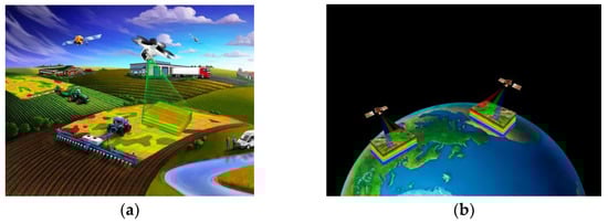
Figure 1. Application of hyperspectral images. (a) Hyperspectral imagery for agricultural applications. (b) Hyperspectral images for Earth observation.

This paper is structured as follows: the second part presents the related work involved in the model proposed in the paper as well as a general introduction to the proposed model; the third part describes the three HSI datasets used for the experiments, the experimental setup, and performance comparison; the fourth part discusses the method of this paper and other comparative methods; the fifth part concludes with conclusions and an implication for future work.

2. Related Work and Method

The method proposed in this paper is a new model of spatial attention network based on 3D OctConv and ViT, and the flow chart of this model is shown in Figure 2. Spatial attention, 3D OctConv, and ViT feature extraction are the three main modules of the framework. This section introduces each of modules separately as well as the model.

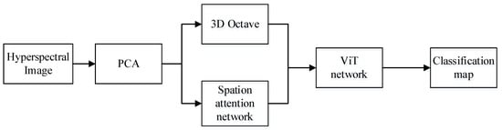
Figure 2. Flow of framework for SATNet.

2.1. D OctConv Module

Since the feature maps generated by CNNs stores its own feature descriptor independently and ignores the common information that could be stored and processed together between adjacent locations, the feature maps have a large amount of redundancy in spatial dimension. In natural images, information is transferred at different frequencies. At the same time, images could be divided into low spatial frequency maps representing global features and high spatial frequency maps representing local features. Similarly, Chen et al. [26] argued that the feature maps generated by CNNs could be decomposed into high-frequency feature maps and low-frequency feature maps by channel and proposed OctConv. OctConv safely reduces the spatial resolution of feature maps and reduces spatial redundant information by sharing information between adjacent locations. Furthermore, it adopts a more efficient inter-frequency information exchange strategy with better performance.

Assuming that X $\in {\mathrm{R}}^{\mathrm{h}\times \mathrm{w}\times \mathrm{c}}$ is the input feature tensor of the convolution layer, where h × w denotes the spatial dimension size and c denotes the spectral dimension size. Along the channel direction, X is decomposed into a high-frequency map ${ \mathrm{X}}^{\mathrm{H}}\in { \mathrm{R}}^{\mathrm{h}\times \mathrm{w}\times (1-\alpha )\mathrm{c}}$ and a low-frequency map X^L$\in {\mathrm{R}}^{\mathrm{h}\times \mathrm{w}\times \alpha \mathrm{c}}$, and the spatial dimension size of the low-frequency map is one-fourth of the original spatial dimension size, where α $\in$ [0, 1] is the proportion of channels assigned to the low-frequency map. To avoid an exhaustive search for the optimal hyperparameter α $\in$ [0, 1], α = 0.5 is chosen in the paper. As shown in Figure 3, the input of the complete OctConv is $\left\{{\mathrm{X}}^{\mathrm{H}},{ \mathrm{X}}^{\mathrm{L}}\right\}$ and the output is $\left\{{\mathrm{Y}}^{\mathrm{H}},{ \mathrm{Y}}^{\mathrm{L}}\right\}$. From ${\mathrm{X}}^{\mathrm{H}}$ to Y^H includes the information update within the high-frequency component ${\mathrm{X}}^{\mathrm{H}->\mathrm{H} }$ and the information exchange between the low-frequency component and the high-frequency component ${\mathrm{X}}^{\mathrm{L}->\mathrm{H}}$. From ${\mathrm{X}}^{\mathrm{L}}$ to Y^L includes the information exchange between the high-frequency component and the low-frequency component ${\mathrm{X}}^{\mathrm{H}->\mathrm{L}}$ and the information update within the low-frequency component ${\mathrm{X}}^{\mathrm{L}->\mathrm{L}}$. The information update within the frequency such as ${\mathrm{X}}^{\mathrm{H}->\mathrm{H} }$ and ${\mathrm{X}}^{\mathrm{L}->\mathrm{L}}$ could be done by the convolution operation only. Y^H is the summation of high frequency component and Y^L is the summation of low frequency component. The equations of Y^H and Y^L are shown below.

$$\begin{array}{ll}{\mathrm{Y}}^{\mathrm{H}}& ={\mathrm{X}}^{\mathrm{H}->\mathrm{H}}{+\mathrm{X}}^{\mathrm{L}->\mathrm{H}}\\ & {=\mathrm{Conv}3\mathrm{d}(\mathrm{X}}^{\mathrm{H}}{;\mathrm{W}}^{\mathrm{H}->\mathrm{H}}{)+\mathrm{up}(\mathrm{Conv}3\mathrm{d}(\mathrm{X}}^{\mathrm{L}}{;\mathrm{W}}^{\mathrm{L}->\mathrm{H}}))\end{array}$$

(1)

$$\begin{array}{ll}{\mathrm{Y}}^{\mathrm{L}}& ={\mathrm{X}}^{\mathrm{H}->\mathrm{L}}{+\mathrm{X}}^{\mathrm{L}->\mathrm{L}}\\ & {=\mathrm{Conv}3\mathrm{d}\left(\mathrm{pool}\right(\mathrm{X}}^{\mathrm{H}}{),\mathrm{W}}^{\mathrm{H}->\mathrm{L} }) +{\mathrm{Conv}3\mathrm{d}(\mathrm{X}}^{\mathrm{L}}{;\mathrm{W}}^{\mathrm{L}->\mathrm{L}})\end{array}$$

(2)

where $\mathrm{Conv}3\mathrm{d}$ denotes 3D convolution, ${\mathrm{W}}^{\mathrm{L}->\mathrm{H}}$ and ${\mathrm{W}}^{\mathrm{H}->\mathrm{L}}$ denotes inter-frequency weight information update,${ \mathrm{W}}^{\mathrm{L}->\mathrm{H}}$ and ${\mathrm{W}}^{\mathrm{H}->\mathrm{L}}$ denotes intra-frequency weight information update, up denotes upsampling operation, and pool denotes downsampling operation.

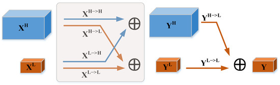
Figure 3. 3D OctConv Module.

Then, to reduce the computational cost, the high-frequency map Y^H of the OctConv output is used to realize the information update from high frequency to low frequency ${\mathrm{Y}}^{\mathrm{H}->\mathrm{L}}$ and the low-frequency map Y^L to realize the information update within low frequency ${\mathrm{Y}}^{\mathrm{L}->\mathrm{L}}$, and then the low-frequency output Y is obtained by joint processing. The formula of Y is as follows.

$$\begin{array}{ll}\mathrm{Y}& ={\mathrm{Y}}^{\mathrm{H}->\mathrm{L}}{+\mathrm{Y}}^{\mathrm{L}->\mathrm{L}}\\ & {=\mathrm{Conv}3\mathrm{d}(\mathrm{pool}(\mathrm{Y}}^{\mathrm{H}}{),\mathrm{W}}^{\mathrm{L}->\mathrm{H}})+{\mathrm{Conv}3\mathrm{d}(\mathrm{Y}}^{\mathrm{L}}{;\mathrm{W}}^{\mathrm{L}->\mathrm{L}})\end{array}$$

(3)

2.2. Spatial Attention Module

Attention mechanisms are processing methods in machine learning that serve to help the networks automatically learn what needs attention in a sequence of text or images. Now they are widely used in tasks such as natural language processing (NLP) and image classification [29]. Attention mechanisms could be divided into channel attention mechanisms, spatial attention mechanisms, and mixed domain attention mechanisms. The channel attention mechanism could adaptively learn the weighting information between different spectral bands to enhance the acquisition of spectral information. The spatial attention mechanism is an adaptive spatial region selection mechanism that could emphasize important pixels in space and suppress useless pixels. The hybrid domain attention mechanism, on the other hand, is a mixture of spectral attention mechanism and spatial attention mechanism, such as the CBAM proposed by Woo et al. [30], which increases the performance capability of the network by integrating the channel attention module and the spatial attention module. Because of the plug-and-play feature and positive effect of the attention modules, the attention modules are also used in the HSI classification task. For example, Zhu et al. [31] proposed a learnable spectral spatial attention module (SSAM), and the SSAM was embedded in the residual block to effectively improve the HSI classification.

A feature map $\mathrm{X}\in {\mathrm{R}}^{\mathrm{h}\times \mathrm{w}\times \mathrm{c}}$ is given as the input to the spatial attention module, where h denotes height, w denotes width, and c denotes channel. To compute spatial attention, first average pooling and maximum pooling operations are performed along the channel axis to obtain feature maps $P_{Avg}\in {\mathrm{R}}^{\mathrm{h}\times \mathrm{w}\times 1}$ and $P_{Max}\in {\mathrm{R}}^{\mathrm{h}\times \mathrm{w}\times 1}$, respectively. Then, they are stitched along the channel axis. Finally, a spatial attention feature map X^′$\in {\mathrm{R}}^{\mathrm{h}\times \mathrm{w}}$ is generated by a convolutional layer with a convolutional kernel size of 7 × 7 and a Sigmoid function. The spatial attention module is shown in Figure 4. The Sigmoid function expression is Equation (4), and the process of X^′ acquisition could be described by Equation (5). Where sig represents the Sigmoid function and f denotes the convolution operation.

$$\mathrm{Sigmoid}\left(\mathrm{x}\right)=\frac{1}{{1+\mathrm{e}}^{-\mathrm{x}}}$$

(4)

$$\begin{array}{ll}{\mathrm{X}}^{\prime }& =\mathrm{sig}(\mathrm{f}([AvgPool(\mathrm{X}),MaxPool(\mathrm{X})]))\\ & =\mathrm{sig}\left(\mathrm{f}\right([P_{Avg},P_{Max}\left]\right))\end{array}$$

(5)

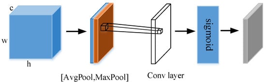
Figure 4. Spatial Attention Module. (Reprinted with permission from Ref. [30]. 2018, Sanghyun Woo, Jongchan Park, Joon-Young Lee, In So Kweon).

2.3. ViT Feature Extraction Module

In recent years, the transformer network [32] has attracted public attention because of its good results in NLP. Inspired by this, the field of computer vision has also started to explore transformer networks. For example, Dosovitskiy et al. [33] were the first to use the transformer model based on the self-attentive mechanism in the field of NLP for image tasks and proposed the vision transformer (ViT) model, and they solved the natural image classification problem from the perspective of sequence data. Because the most important self-attention mechanism in transformer enables the ViT model to extract the global features of feature maps, the transformer network is considered promising for many tasks. Currently, numerous scholars have applied the transformer model to HSI classification tasks. In order to improve the performance of HSI classification from the perspective of spatial structure, Zhao et al. [34] proposed the convolutional transformer network (CTN), which used a two-dimensional center position encoding rather than a one-dimensional sequence position encoding. They also introduced the convolutional transformer block (CT), which combined the convolutional and transformer structures to capture local and global features of HSI. Hong et al. [35] proposed a SpectralFormer network to process continuous spectral information using the transformer to achieve HSI classification from the perspective of spectral sequences.

Unlike the standard transformer model, the input of ViT model is not a one-dimensional sequence, but a series of flattened patches X_p$\in {\mathrm{R}}^{{\mathrm{n}\times \mathrm{p}}^2\times \mathrm{c}}$ divided by a two-dimensional image $\mathrm{X}\in {\mathrm{R}}^{\mathrm{h}\times \mathrm{w}\times \mathrm{c}}$, where h $\times$ w is the image size, p $\times$ p is the patch size, and $\mathrm{n}=\frac{\mathrm{h}\times \mathrm{w}}{{\mathrm{p}}^2}$ is the number of patches, which is also the length of the ViT input sequence. Then, a one-dimensional patch embedding is obtained by linear transformation, and to ensure that the input is the original image. Therefore, a position embedding is introduced to determine the order of each patch. A token is obtained by adding the position vector to the patch embedding and inputting the token into the Transformer Encoder, which is shown in Figure 5. Encoder is the core part of the ViT model, which consists of a normalization layer, a multi-headed self-attention layer, a residual connection, and an MLP layer. The normalization layer needs to be added before each multi-headed attention layer and MLP, and after it in residual concatenation. Among them, the most critical part of Transformer Encoder is the multi-headed self-attentive layer, which could capture the internal correlation of features and thus reduce the dependence on external information. The process of implementing the multi-headed self-attentive layer is as follows.

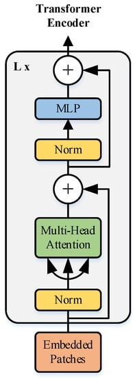
Figure 5. Transformer Encoder Module. (Reprinted with permission from Ref. [33]. 2021, Alesey Dosovitskiy, Lucas Beyer, Alexander Kolesnikov, Dirk Weissenborn, Xiaohua Zhai, Thomas Unterthiner, Mostafa Dehghani, Matthias Minderer, Georg Heigold, Sylvain Gelly, Jakob Uszkoreit, Neil Houlsby.)

(i)

Input sequence data ${\mathrm{x}}_1{, \mathrm{x}}_2{, \mathrm{x}}_3, \cdots {, \mathrm{x}}_{\mathrm{t}}$, where ${\mathrm{x}}_{\mathrm{i}}$(i = 1, …, t) denote the vector.

(ii)

The initial embedding is performed by embedding layer to get ${\mathrm{a}}_1{, \mathrm{a}}_2{, \mathrm{a}}_3, \cdots {, \mathrm{a}}_{\mathrm{t}}$, ${\mathrm{a}}_{\mathrm{i}}=\mathrm{W}·{\mathrm{x}}_{\mathrm{i}}$, where W is the shared matrix.

(iii)

Multiplying each by three different matrices W_q, W_k and W_v, respectively, three vectors Query $\left(\mathrm{Q}=\left[{\mathrm{q}}_{1,}\cdots {,\mathrm{q}}_{\mathrm{t}}\right]\right)$, Key $\left(\mathrm{K}=\left[{\mathrm{k}}_{1,}\cdots {, \mathrm{k}}_{\mathrm{t}}\right]\right)$ and Value $\left(\mathrm{V}=\left[{\mathrm{v}}_{1,}\cdots {, \mathrm{v}}_{\mathrm{t}}\right]\right)$ could be obtained.

(iv)

The attention score S is obtained by inner product of each Q and each K, for example. To make the gradient stable, the attention score is normalized. Such as ${\mathrm{S}}_{\mathrm{i},\mathrm{j}}{=\mathrm{q}}_{\mathrm{i}}·{\mathrm{k}}_{\mathrm{j}}∕\sqrt{\mathrm{d}}$, d is the dimension of ${\mathrm{q}}_{\mathrm{i}}$ or ${ \mathrm{k}}_{\mathrm{j}}$.

(v)

Performing the Softmax function on S, we get as ${\mathrm{s}}_{1,\mathrm{j}}=\frac{{\mathrm{e}}^{{\mathrm{S}}_{1,\mathrm{i}}}}{{\sum }_{\mathrm{j}}{\mathrm{e}}^{{\mathrm{S}}_{1,\mathrm{j}}}}$. The Softmax function is defined as follows:

$${\mathrm{Softmax}(\mathrm{Z}}_{\mathrm{i}})=\frac{{\mathrm{e}}^{{\mathrm{Z}}_{\mathrm{i}}}}{{\mathsf{\Sigma }}_{\mathrm{C}=1}^{\mathrm{C}}{\mathrm{e}}^{{\mathrm{z}}_{\mathrm{c}}}}$$

(6)

(vi)

Finally, an attention matrix $\mathrm{Z}=\left[{\mathrm{Z}}_1,\cdots {,\mathrm{Z}}_{\mathrm{m}}\right] \mathrm{is} \mathrm{generated}$, where ${\mathrm{Z}}_{\mathrm{i}}=\sum {\mathrm{s}}_{1,\mathrm{i}}{\mathrm{v}}_{\mathrm{i}}$. In summary, the multi-headed attention mechanism could be expressed as

$$\mathrm{Z}=\mathrm{Attention}(\mathrm{Q},\mathrm{K},\mathrm{V})=\mathrm{Softmax}\left(\frac{{\mathrm{QK}}^{\mathrm{T}}}{\sqrt{\mathrm{d}}}\right)\mathrm{V}$$

(7)

The above Equation (7) allows combining several different multi-headed self-attentive layers into one multi-headed attention (e.g., h = 3) denoted as M_h, h = 1, …, 3, and stitching them together first and last to make the feature dimension the same as the input data using linear transformation. The self-attention mechanism pseudo-code is shown in Algorithm 1.

Algorithm 1 Self-Attention

Input: Input sequence $\mathrm{X}=\left[{\mathrm{x}}_1{, \mathrm{x}}_2, \cdots {,\mathrm{x}}_{\mathrm{t}}\right]$

Output: Attention Matrix $\mathrm{Z}=\left[{\mathrm{Z}}_1,\cdots {,\mathrm{Z}}_{\mathrm{t}}\right]$

1. $\mathrm{A} \leftarrow \mathrm{W}·\mathrm{X}$; // A is the characteristic matrix, W for shared matrix 2. $\mathrm{Q} \leftarrow { \mathrm{W}}_{\mathrm{q}}·\mathrm{A}$; // $\mathrm{Q}=\left[{\mathrm{q}}_{1,}\cdots ,{\mathrm{q}}_{\mathrm{t}}\right]$$, {\mathrm{W}}_{\mathrm{q}}$ is a matrix 3. $\mathrm{K} \leftarrow { \mathrm{W}}_{\mathrm{k}}·\mathrm{A}$; // $\mathrm{K}=\left[{\mathrm{k}}_{1,}\cdots ,{\mathrm{k}}_{\mathrm{t}}\right]$, Wk is a matrix 4. $\mathrm{V} \leftarrow { \mathrm{W}}_{\mathrm{v}}·\mathrm{A}$; // $\mathrm{V}=\left[{\mathrm{v}}_{1,}\cdots ,{\mathrm{v}}_{\mathrm{t}}\right]$$, {\mathrm{W}}_{\mathrm{v}}$ is a matrix 5. for$\mathrm{i} \leftarrow$0 to t − 1 do 6. for$\mathrm{j} \leftarrow$0 to t − 1 do 7. Si,j $\leftarrow$$\mathrm{Softmax}\left(\right({\mathrm{q}}_{\mathrm{i}}$·${\mathrm{k}}_{\mathrm{j}}$)/$\sqrt{\mathrm{d}}$) according to Equation (6); // $\mathrm{d} \mathrm{is} \mathrm{the} \mathrm{dimension} \mathrm{of} {\mathrm{q}}_{\mathrm{i}} \mathrm{o}\mathrm{r}$ ${\mathrm{k}}_{\mathrm{j}}$ 8. end for 9. end for 10. for i $\leftarrow$0 to t − 1 do 11. for j $\leftarrow$0 to t − 1 do 12. ${\mathrm{Z}}_{\mathrm{i}}\leftarrow \sum {\mathrm{S}}_{\mathrm{i},\mathrm{j}}·{\mathrm{v}}_{\mathrm{i}}$ 13. end for 14. end for 15. $\mathrm{return} \mathrm{Z}=\left[{\mathrm{Z}}_1,\cdots {,\mathrm{Z}}_{\mathrm{t}}\right]$;

2.4. Method

The method proposed in this paper was a new model of spatial attention network based on 3D OctConv and ViT, as shown in Figure 6. Assuming that the HSI cube data input to the model was M $\in {\mathrm{R}}^{\mathrm{H}\times \mathrm{W}\times \mathrm{C}}$, we first used PCA for M to reduce the spectral redundancy and thus the spectral dimension size. The reduced dimensionality results in an HSI cube of M^′$\in {\mathrm{R}}^{\mathrm{H}\times \mathrm{W}\times \mathrm{C}}$. The number of spectral bands was reduced from the original C to B. Then, M^′ is divided into multiple 3D-patches, and the label of each patch is determined by the label of its central pixel. The divided patches are noted as $\mathrm{X} \in { \mathrm{R}}^{\mathrm{S}\times \mathrm{S}\times \mathrm{B}}$, where $\mathrm{S} \times \mathrm{S}$ denotes the spatial size of the patches and B is the number of spectral bands. In order to make full use of the label information of HSI, the overlapping patches are taken as the input of the model in this paper.

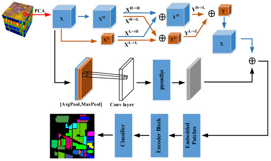
Figure 6. Spatial attention network structure combining 3D Octave convolution and ViT.

The OctConv module in this paper consists of two 3D Octave convolutions. The first one is a simple Octave convolution whose input is $\left\{\mathrm{X}, 0\right\}$ and output is $\left\{{\mathrm{X}}^{\mathrm{H}}{, \mathrm{X}}^{\mathrm{L}}\right\}$. X is considered as the high-frequency component of OctConv and the low-frequency component is 0. ${\mathrm{X}}^{\mathrm{H}}$ could be considered as the result of updating the high-frequency information of the high-frequency component X and adding 0. Then, additionally, ${\mathrm{X}}^{\mathrm{L}}$ is the result of the information exchange between the high-frequency and low-frequency of the high-frequency component X and the summation of 0. In the intra-frequency update and inter-frequency exchange of the spatial information of X, we also divide the channel information, and the number of channels of the high-frequency component and the low-frequency component is half of the original one, and the obtained high-frequency component is ${ \mathrm{X}}^{\mathrm{H}} \in { \mathrm{R}}^{\mathrm{S}\times \mathrm{S}\times \frac{\mathrm{B}}{2}}$ and the low-frequency component is ${\mathrm{X}}^{\mathrm{L}} \in { \mathrm{R}}^{\frac{\mathrm{S}}{2}\times \frac{\mathrm{S}}{2}\times \frac{\mathrm{B}}{2}}$. The second one is a complete Octave convolution, whose input is $\left\{{\mathrm{X}}^{\mathrm{H}}{, \mathrm{X}}^{\mathrm{L}}\right\}$ and output is $\left\{{\mathrm{Y}}^{\mathrm{H}}{, \mathrm{Y}}^{\mathrm{L}}\right\}$. It consists of four branches, which could be described in detail in Section 2.1 above. The Octave convolution obtains the new high-frequency component Y^H$\in { \mathrm{R}}^{\mathrm{S}\times \mathrm{S}\times \frac{\mathrm{B}}{2}}$ and the low-frequency component ${\mathrm{Y}}^{\mathrm{L}}\in { \mathrm{R}}^{\frac{\mathrm{S}}{2}\times \frac{\mathrm{S}}{2}\times \frac{\mathrm{B}}{2}}$ by constructing inter-frequency and intra-frequency information communication mechanisms for X^H and X^L, respectively. Then, a down-sampling and convolution operation is performed on Y^H for inter-frequency information update ${\mathrm{Y}}^{\mathrm{H}->\mathrm{L}}$, and a convolution operation is performed on Y^L for intra-frequency information exchange ${\mathrm{Y}}^{\mathrm{L}->\mathrm{L}}$. Finally, along the channel direction, ${\mathrm{Y}}^{\mathrm{H}->\mathrm{L}}$ and ${\mathrm{Y}}^{\mathrm{L}->\mathrm{L}}$ are combined to obtain a new low-frequency component Y $\in { \mathrm{R}}^{\frac{\mathrm{S}}{2}\times \frac{\mathrm{S}}{2}\times \mathrm{B}}$.

In the above, we utilize Octave convolution to reduce the redundancy of spatial information. In addition, we use the spatial attention mechanism for X at the same time to establish the spatial correlation of different features. In order to avoid the input patch of ViT module being too small and increasing the length of the input sequence, the result of the spatial attention mechanism is summed with Y and up-sampling to obtain Z, which has the same spatial size as that of X. Along the channel direction, the summed Z is transformed into 2D data and then the Patch Embedding is obtained by a one-dimensional linear transformation. In addition, the Patch embedding is fed into the Transformer Encoder module with the position vector, and the global features are obtained by the ViT network module. Finally, a fully connected layer is used to classify the different pixels to obtain the final classification results.

3. Experiments

To evaluate the performance of the algorithms, the experiments in the paper were mainly done on a computer with a processor of Inter(R) Core(TM) i9-10900k @3.70 GHz, 32G RAM, and a graphics card of NVIDIA GeForce RTX 3090 (32G RAM). The software environment was Ubuntu 20.4 under Linux, the deep learning framework used was Pytorch 1.10, and the programming language was python 3.8.

In this part, we organized the model’s hyperparameters and measured the model’s classification accuracy using three widely used assessment metrics: overall classification accuracy (OA), average classification accuracy (AA), and Kappa coefficient (Kappa) [36]. OA is the ratio of the number of correct classifications in the sample to the total number of samples; AA is the number of correct predictions in each category divided by the total number of that category, and then averaged for each category; Kappa coefficient is an index used for consistency testing, and its value range is [−1, 1]. To verify the classification effectiveness of the method in the paper, experiments are conducted on three publicly available datasets, India Pines (IP), Pavia University (UP), and Salinas (SA).

3.1. Data Description

The following describes the information related to the three publicly available datasets used, with the number of each category in each dataset shown in Table 1, Table 2 and Table 3.

Table 1. Number of training and testing samples for the India Pines dataset.

Number	Class Name	Train	Test	Total
1	Alfalfa	5	41	46
2	Corn-notill	143	1285	1428
3	Corn-min	83	747	830
4	Corn	24	213	237
5	Grass-pasture	48	435	483
6	Grass-trees	73	657	730
7	Grass-pasture-mowed	3	25	28
8	Hay-windrowed	48	430	478
9	Oats	2	18	20
10	Soybean-notill	97	875	972
11	Soybean-mintill	245	2210	2455
12	Soybean-clean	59	534	593
13	Wheat	20	185	205
14	Woods	126	1139	1265
15	Buildings-Grass-Trees	39	347	386
16	Stone-Steel-Tosers	9	84	93
Total Samples		1024	9225	10,249

Table 2. Number of training and testing samples for the Pavia University dataset.

Number	Class Name	Train	Test	Total
1	Asphalt	332	6299	6631
2	Meadows	932	17,717	18,649
3	Gravel	105	1994	2099
4	Trees	153	2911	3064
5	Painted metal sheets	67	1278	1345
6	Bare soil	251	4778	5029
7	Bitumen	67	1263	1330
8	Self-Blocking bricks	184	3499	3683
9	Shadows	47	900	947
Total Samples		2138	40,638	42,776

Table 3. Number of training and testing samples for the Salinas dataset.

Number	Class Name	Train	Test	Total
1	Broccoli_green_weeds_1	100	1909	2009
2	Broccoli_green_weeds_2	186	3540	3726
3	Fallow	99	1877	1976
4	Fallow_rough_plow	70	1324	1394
5	Fallow_smooth	134	2544	2678
6	Stubble	198	3761	3959
7	Celery	179	3400	3579
8	Grapes_untrained	564	10,707	11,271
9	Soil_vinyard_develop	310	5893	6203
10	Com_senesces_green_weeds	164	3114	3278
11	Lettuce_romaine_4wk	53	1015	1068
12	Lettuce_romaine_5wk	96	1831	1927
13	Lettuce_romaine_6wk	46	870	916
14	Lettuce_romaine_7wk	54	1016	1070
15	Vinyard_untrained	363	6905	7268
16	Vinyard_untrained_trellis	90	1717	1807
Total Samples		2706	51,423	54,129

1.

India Pines (IP): It was taken by the airborne sensor AVIRIS in the agricultural area of northwestern Indiana, USA. The image has a spatial size of $145 \times 145$, a spatial resolution of roughly 20 m, and a wavelength range of 400–2500 nm. Additionally, there are 200 effective spectral bands, which were divided into 16 feature classes. During the experiment, 10% of the samples in each category were randomly selected as the training set, and the remaining samples were used as the test set. The detailed division results are shown in Table 1.

2.

Pavia University (UP): It was acquired by the airborne sensor ROSIS in the area of the University of Pavia, Northern Italy. The image has a spatial size of $610 \times 340$, a spatial resolution of roughly 1.3 m, and a wavelength range of 430–860 nm. There are 103 effective spectral bands of the image, and it has 9 feature classes in total. During the experiment, 5% of the samples in each category were randomly selected as the training set, and the remaining samples were used as the test set. The detailed division results are shown in Table 2.

3.

Salinas (SA): It was acquired by the airborne sensor AVIRIS in Salinas Valley, California, USA. The image has a spatial size of $512 \times 217$, a spatial resolution of roughly 3.7 m, and a wavelength range of 360–2500 nm. Additionally, there are 204 effective spectral bands, which were divided into 16 feature classes. During the experiment, 5% of the samples in each category were randomly selected as the training set, and the remaining samples were used as the test set. The detailed division results are shown in Table 3.

3.2. Parameter Setting

All experiments in the paper set the epoch size to 100, the batch size to 32, and the patch size to $15 \times 15$. The classification performance is shown in Figure 7 to be at its best when the spectral bands of IP, UP, and SA are taken as 110, 30, and 30, respectively, taking into account the integrated OA and training duration. Therefore, the number of principal components set for the three datasets IP, UP, and SA are 110, 30, and 30, respectively. The Octave convolution module has three convolutional layers, using eight $3 \times 3 \times 3$ 3D convolutional kernels, 16 $3 \times 3 \times 3$ 3D convolution kernels and 32 3 × 3 × 3 3D convolution kernels. In the first convolutional layer, there are two branches, which are information updates between high frequency and within high frequency and information updates between high frequency and low frequency by downsampling. In the second convolutional layer, there are four branches, which are information updates between high frequency and within high frequency, information exchange between high frequency and low frequency, information update between low frequency and high frequency, and information update between low frequency and within low frequency by upsampling. In the third convolutional layer, information is exchanged between low and high frequencies and information is updated between low and low frequencies. Finally, a low frequency component is obtained. As the depth of the network increased, the problem of gradient disappearance tended to occur. Therefore, we invoke batch normalization in the 3D OctConv module to avoid gradient disappearance. During the experiment, the dependence between neurons easily leads to overfitting of the neural network during the training process, which has an impact on the experimental results. In addition, the speed of parameter movement to the optimal value also affects the experimental results. In order to obtain the best experimental results, the settings of the hyperparameters dropout rate and learning rate size are explored in this paper.

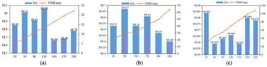
Figure 7. Comparison plots of OA and runtime when using different numbers of spectral bands on different datasets: (a) IP dataset; (b) UP dataset; (c) SA dataset.

4.

The different values of dropout rate setting would affect the experimental results. After setting the dropout rate, some neurons would be stopped during training, but no neurons would be discarded during testing. Therefore, setting a reasonable dropout rate is helpful to improve the stability and robustness of the model and prevent overfitting. The range of values of dropout was [0.1, 0.2, 0.3, 0.4, 0.5, 0.6, 0.7, 0.8, 0.9, 1.0], and we compared different dropouts chosen for three data sets, respectively. The classification results of different dropout sizes were shown in Table 4. From Table 4, we could see that for the IP dataset, when the dropout value was set to 0.3, the OA was the maximum value, and the classification performance was the best. For the UP dataset, when the dropout value was set to 0.4, the OA was the maximum value, and the classification performance was the best. For the SA dataset, when the dropout value was set to 0.9, the OA was the maximum value, and the classification performance was the best.

Table 4. Different dropout rates.

Dropout Rate	0.1	0.2	0.3	0.4	0.5	0.6	0.7	0.8	0.9
IP(OA/%)	98.79	98.60	99.06	98.97	98.85	99.02	98.71	98.85	98.72
UP(OA/%)	99.65	99.59	99.52	99.67	99.57	99.45	99.62	99.58	98.64
SA(OA/%)	99.97	99.96	99.96	99.97	99.93	99.97	99.97	99.96	99.98

5.

The tuning of the learning rate has an important impact on the performance of the network model. If the learning rate is too large, it would cause the training cycle to oscillate and is likely to cross the optimal value. Conversely, the optimization efficiency may be too low, leading to a long time without convergence. In this paper, a grid search method was used to find the optimal learning rate from [0.01, 0.005, 0.001, 0.0005, 0.0001, 0.00005] for experiments. The classification results of different learning rate sizes were shown in Table 5. From Table 5, it could be seen that for the IP dataset, when the learning rate was set to 0.001, the OA at this time was the maximum value and the classification performance was the best. For the UP dataset, when the learning rate was set to 0.00005, the OA at this time was the maximum value and the classification performance was the best. For the SA dataset, when the learning rate was set to 0.0001, the OA at this time was the maximum value and the classification performance is the best.

Table 5. Different learning rates.

Learning Rate	0.01	0.005	0.001	0.0005	0.0001	0.00005
IP(OA/%)	92.325	98.569	99.06	98.785	98.916	98.959
UP(OA/%)	94.918	98.983	99.552	99.456	99.542	99.670
SA(OA/%)	53.866	86.684	99.928	99.945	99.984	99.929

3.3. Performance Comparison

The first experiment used the IP dataset, 10% of each type of data was randomly selected as training data, and the rest was used as test data. The total number of training samples was 9225. The UP dataset was utilized in the second experiment; 5% of each category of data was randomly chosen as training data, and the remaining data was used as test data. There were a total of 2138 training samples in this experiment. The SA dataset was utilized in the third experiment; a total of 2706 training samples were used, with 5% of each category of data randomly chosen as training data and the remaining data used as test data. In order to verify the effectiveness of the algorithm in the paper, the experiments were compared with some traditional methods and mainstream deep learning methods such as Baseline, SSRN [37], 3DCNN [38], and HybridSN [39]. Additionally, ablation experiments were carried out in this research, and the approaches used were contrasted with network that only used the ViT model (ViT model), network that only used 3D OctConv (3D_Octave model), and network that only used 3D OctConv in conjunction with ViT (OctaveVit model). The experimental results were shown in Table 6, Table 7 and Table 8.

Table 6. Test accuracy with different preprocessing methods on the IP dataset.

Class No.	Baseline	3DCNN	SSRN	HybridSN	ViT	3D_Octave	OctaveVit	SATNet
1	100.00	100.00	100.00	96.55	100.00	88.89	100.00	100.00
2	92.74	93.13	97.93	99.84	91.63	99.20	98.76	99.45
3	81.01	88.41	95.72	97.63	88.82	98.93	99.34	99.73
4	78.29	100.00	100.00	100.00	95.50	98.12	100.00	98.16
5	99.02	97.76	98.85	95.34	99.31	100.00	98.64	99.77
6	97.14	98.92	100.00	99.39	98.34	98.77	98.95	99.55
7	85.71	100.00	100.00	91.30	100.00	100.00	100.00	100.00
8	86.44	99.88	100.00	100.00	94.71	99.77	100.00	100.00
9	33.33	100.00	100.00	100.00	84.21	100.00	100.00	100.00
10	91.16	94.28	94.58	96.66	97.11	97.32	99.18	98.85
11	94.42	95.47	96.20	98.65	93.16	98.74	99.28	98.88
12	86.99	94.56	98.83	96.34	92.52	98.28	97.35	97.04
13	100.00	100.00	100.00	95.48	100.00	98.93	100.00	98.93
14	98.24	96.53	99.56	99.56	98.94	99.04	99.74	99.82
15	87.06	99.68	100.00	98.30	91.06	98.86	98.29	98.30
16	91.67	96.77	98.46	91.03	93.42	86.67	90.12	88.31
OA(%)	92.00	95.64	97.48	98.33	93.89	98.63	99.04	99.06
AA(%)	78.29	90.23	95.44	91.30	82.50	98.14	98.56	98.35
Kappa(%)	90.89	95.01	97.12	98.09	93.01	98.44	98.91	98.92

Table 7. Test accuracy with different preprocessing methods on the UP dataset.

Class No.	Baseline	3DCNN	SSRN	HybridSN	ViT	3D_Octave	OctaveVit	SATNet
1	96.74	96.27	98.88	99.33	92.12	99.41	99.81	99.81
2	98.50	99.33	98.98	99.94	96.48	99.97	99.99	99.95
3	86.68	96.25	96.32	98.30	85.57	99.09	99.39	99.30
4	98.38	98.64	86.30	98.76	98.15	98.83	98.45	99.30
5	100.00	100.00	100.00	99.69	100.00	100.00	100.00	100.00
6	99.76	98.34	99.98	99.65	96.63	98.83	99.94	100.00
7	95.94	99.92	100.00	99.92	90.33	99.45	99.53	99.68
8	89.97	93.65	99.16	96.56	88.77	97.51	98.08	98.67
9	99.29	98.96	97.69	98.11	97.30	99.21	98.43	97.68
OA (%)	97.01	98.08	97.94	99.30	94.70	99.49	99.60	99.67
AA (%)	95.43	97.09	98.36	98.81	91.27	99.17	99.14	99.33
Kappa (%)	96.02	97.45	97.28	99.08	92.93	99.33	99.47	99.56

Table 8. Test accuracy with different preprocessing methods on the SA dataset.

Class No.	Baseline	3DCNN	SSRN	HybridSN	ViT	3D_Octave	OctaveVit	SATNet
1	100.00	100.00	40.25	100.00	99.90	99.95	100.00	100.00
2	100.00	100.00	100.00	100.00	99.66	100.00	100.00	100.00
3	100.00	100.00	81.05	100.00	92.78	100.00	100.00	100.00
4	100.00	98.65	80.51	100.00	99.74	100.00	99.92	99.92
5	99.45	99.92	94.91	99.96	82.27	100.00	99.76	99.80
6	100.00	100.00	98.77	99.92	100.00	100.00	99.97	99.80
7	100.00	100.00	100.00	100.00	99.94	100.00	100.00	99.97
8	98.52	99.10	85.58	99.93	91.26	99.81	100.00	100.00
9	99.86	100.00	87.66	100.00	99.88	100.00	100.00	100.00
10	99.94	99.62	90.63	99.68	99.58	99.81	99.97	99.98
11	99.61	99.90	89.39	99.80	100.00	100.00	100.00	100.00
12	99.62	100.00	91.42	100.00	96.52	100.00	100.00	100.00
13	99.42	98.31	98.74	100.00	96.19	99.89	99.89	100.00
14	100.00	100.00	100.00	98.72	99.76	100.00	100.00	100.00
15	97.61	97.22	82.64	99.90	81.57	99.99	100.00	100.00
16	100.00	100.00	96.32	100.00	73.75	100.00	100.00	100.00
OA (%)	99.29	99.33	84.97	99.91	92.81	99.94	99.980	99.984
AA (%)	99.57	99.40	85.55	99.87	90.58	99.93	99.970	99.979
Kappa (%)	99.21	99.26	83.28	99.90	92.00	99.94	99.978	99.982

It could be seen from the IP dataset (Table 6) that Baseline had the worst classification performance, and the method in this paper improved 7.06, 3.42, 1.58, 0.73, 5.17, 0.43, 0.02 compared to Baseline, 3DCNN, SSRN, HybridSN, ViT, 3D_Octave, and OctaveVit on OA; improved 20.06, 8.12, 2.91, 7.05, 15.85, 0.21, −0.21 on AA; improved 8.03, 3.91, 1.8, 0.83, 5.91, 0.48, 0.01 on Kappa coefficient, respectively. In addition, it could be found that the OA of the Class I, Class VII, Class IX, and Class XIII of the IP dataset were higher than the other categories and easier to distinguish. From the UP dataset (Table 7), it could be seen that the method in this paper improved 2.66, 1.59, 1.73, 0.37, 4.97, 0.18, 0.07, compared with Baseline, 3DCNN, SSRN, HybridSN, ViT, 3D_Octave, and OctaveVit on OA; and on AA improved by 3.9, 2.24, 0.97, 0.52, 8.06, 0.16, 0.19, respectively; on Kappa coefficient improved by 3.54, 2.11, 2.28, 0.48, 6.63, 0.23, 0.09, respectively. In addition, it could be found that the overall classification accuracy of the Class V of the UP dataset was higher and less difficult to distinguish than the other categories. From the SA dataset (Table 8), it could be seen that the method in this paper improved 0.694, 0.654, 15.014, 0.074, 7.174, 0.044, 0.004 on OA compared with Baseline, 3DCNN, SSRN, HybridSN, ViT, 3D_Octave, and OctaveVit, respectively; on AA it improved by 0.409, 0.579, 14.429, 0.109, 9.399, 0.049, 0.009; on Kappa coefficients improved by 0.772, 0.722, 16.702, 0.082, 7.982, 0.042, 0.004, respectively. From the results in the table, we could find that SA classification accuracy was generally higher than IP and UP, and the classification difficulty was lower, in which the classification accuracy of the Class V and Class X of SA was lower and the classification difficulty is a bit more. From these tables, they could be shown that with limited training samples, the classification accuracy of the models proposed in the paper could be found to be better than other models by comparison. The performance of the 3DCNN classification model is better than that of the Baseline classification model because the 3D convolution kernel could extract features of 3D data more in line with the characteristics of hyperspectral data in three dimensions [40]. While combining 3D convolution, which could extract spectral-spectral features, and 2D convolution, which could extract spatial features, learn a more abstract spatial representation, and reduce the model complexity, the HybridSN model’s classification performance was better than the 3DCNN and SSRN. The 3D_Octave model outperformed the ViT model in classification, while the OctaveVit outperformed the 3D_Octave in classification on the IP and UP datasets. As indicated in Table 9, we also contrasted the computational complexity and quantity of model parametrizations for various techniques on various datasets. According to the table, Baseline employing only the completely connected layer has the most model parameters, followed by 3D Octave, HybridSN, and SATNet. Due to its utilization of all spectral bands, SSRN requires the most computational effort. On the IP dataset, HybridSN required more computational effort than SATNet, while on the UP and SA datasets, SATNet required more computational effort than HybridSN. Additionally, 3D Octave required less processing power than HybridSN, since it divided the feature maps into frequency-based components.

Table 9. Complexity and number of parameters of different algorithms.

	IP		UP		SA
	GFLOPs	Params	GFLOPs	Params	GFLOPs	Params
Baseline	2.16	67.5M	0.98	30.6M	0.98	30.6M
3DCNN	0.187	0.82M	0.043	0.11M	0.459	0.20M
SSRN	14.19	0.34M	7.29	0.19M	14.47	0.35M
HybridSN	8.88	2.67M	1.70	1.19M	1.70	1.19M
ViT	0.0726	1.9M	0.0357	0.8M	0.0357	0.8M
3D_Octave	5.46	22.1M	1.489	6.06M	1.489	6.06M
OctaveVit	6.81	2.41M	2.10	0.93M	2.10	0.93M
SATNet	7.89	2.40M	2.40	0.93M	2.40	0.93M

From the above results, it could be concluded that all three metrics (OA, AA, and Kappa) reflected that the classification performance of our method on these three datasets was significantly better than other methods. To comprehensively evaluate the classification performance, Figure 8, Figure 9 and Figure 10 showed the classification graphs obtained using different methods on the three datasets of IP, UP, and SA, respectively, from a visualization perspective. The comparison showed that on the IP dataset, the classification map of Baseline produced the most noise points and many pixels were misclassified on the boundary between different categories, followed by the classification maps of 3DCNN and ViT with more noise points. The classification map of this paper’s method had the least noise points and had clearer discrimination, despite OctaveVit and 3D_Octave having fewer noise points. Since the spatial resolution of the IP dataset is larger than that of the UP and SA datasets, it is easier to produce mixed image elements and more difficult to classify. Therefore, the classification map of the UP and SA datasets produced fewer noise points than those of the IP dataset. On the UP dataset, the classification map of ViT produced the most noise points and the largest error. While the classification map of the method in this paper has the highest quality and the least number of misclassified pixel points, OctaveVit and 3D_Octave are only the second highest. For the classification maps of SA dataset, the classification map of SSRN produced the most noise points and the worst classification effect, followed by ViT, Baseline, and 3DCNN. OctaveVit and 3D_Octave classification maps have fewer noise points, and the classification map of the proposed method in this paper had the least noise points and was closest to ground truth map.

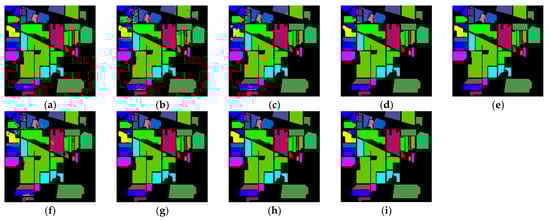
Figure 8. Classification maps generated by all of the competing methods on the Indian Pines data with 10% training samples; (a) is ground truth map, and (b–i) are the results of Baseline, 3DCNN, SSRN, HybridSN, ViT, 3D_Octave, OctaveVit, SATNet, respectively.

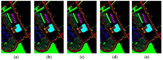
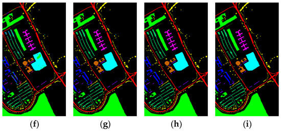
Figure 9. Classification maps generated by all of the competing methods on the University of Pavia data with 5% training samples; (a) is ground truth map, and (b–i) are the results of Baseline, 3DCNN, SSRN, HybridSN, ViT, 3D_Octave, OctaveVit, SATNet, respectively.

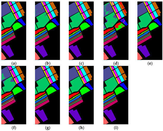
Figure 10. Classification maps generated by all of the competing methods on the Salinas Scene data with 5% training samples; (a) is ground truth map, and (b–i) are the results of Baseline, 3DCNN, SSRN, HybridSN, ViT, 3D_Octave, OctaveVit, and SATNet, respectively.

Figure 11, Figure 12 and Figure 13 showed the confusion matrixes obtained on the IP, UP, and SA datasets using different methods such as Baseline, 3DCNN, SSRN, HybridSN, ViT, 3D_Octave, and OctaveVit, respectively. Each row of it represented the predicted value, each column represented the actual value, and the value on the diagonal line represented the correctly predicted result. The confusion matrix provided an intuitive view of the performance of the classification algorithm on each category. It put the predicted and true results of each category in a table, so that the number of correct and incorrect identifications for each category could be clearly known. For the IP dataset, it could be seen from Figure 11h that there are 22 Class II features predicted as the Class XI, and 16 Class XVI features predicted as the Class XII. For the UP dataset, it could be seen from Figure 12h that 11 Class I features are predicted as Class VIII and 6 Class IV features are predicted as Class I. In addition, 11 Class III features are predicted as Class VIII and, 26 Class IV features are predicted as Class VIII; 15 Class VIII features are predicted as Class IV, indicating that Class I, Class III, and Class IV features are not easily distinguished from Class VIII distinction. For the SA dataset, it could be seen from Figure 13h that 3 Class VI features were predicted as Class V; 2 Class IV features were predicted as Class V.

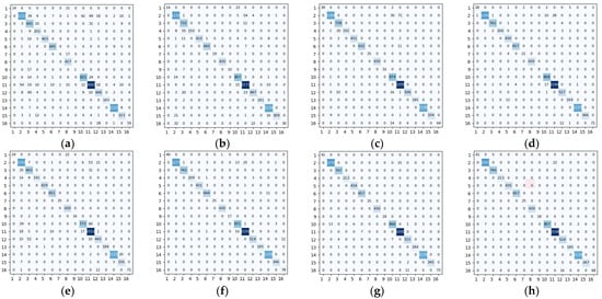
Figure 11. Confusion matrix of different methods for the Indian Pines data set. (a) Baseline (b) 3DCNN (c) SSRN (d) HybridSN (e) ViT (f) 3D_Octave (g) OctaveVit (h) SATNet.

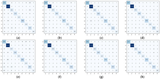
Figure 12. Confusion matrix of different methods for the University of Pavia data set. (a) Baseline (b) 3DCNN (c) SSRN (d) HybridSN (e) ViT (f) 3D_Octave (g) OctaveVit (h) SATNet.

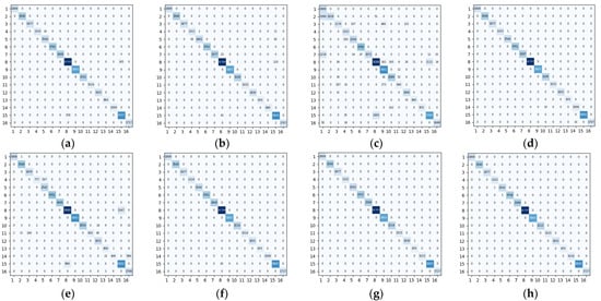
Figure 13. Confusion matrix of different methods for the Salinas Scene data set. (a) Baseline (b) 3DCNN (c) SSRN (d) HybridSN (e) ViT (f) 3D_Octave (g) OctaveVit (h) SATNet.

4. Discussion

Based on our experimental results on three publicly available datasets, it showed the superiority of our method over other methods. The ViT method only used Vision Transformer for HSI classification. From the results in Table 6, Table 7 and Table 8, we could find that it had a certain gap compared with the results of our method. Since the attention mechanism concentrates on important information while ignoring secondary information, ViT model training necessitates a large amount of data. Therefore, when there are few samples available for the HSI classification task, the VIT model’s classification performance falls. 3D_Octave method was to classify HSI using only 3D OctConv. From the classification results, the classification performance of 3D_Octave method was better than ViT method, because 3D_Octave could extract the spectral-spatial information of HSI, while the ViT model extracted the spatial information. The classification performance of the OctaveVit method outperformed the 3D_Octave method on the IP and UP datasets, and is slightly inferior on the SA dataset. Although the technique in this article outperformed the OctaveVit method in terms of classification performance, the classification performance gap was not very wide, which supports the efficiency of the spatial attention mechanism we employ. According to the results of ablation experiments, the method we proposed has superiority, but there are still shortcomings: (1) when the HSI spatial resolution of the model input is high, increasing the length of the input sequence to ViT would slow down the model’s training and inference speeds; (2) the number of samples will also affect the model’s classification effect, but there are only a finite number of HSI labeled samples. To address these problems, we could try to improve the ViT model in the future and think about reducing the complexity of the self-attentive mechanism from the lightweight perspective.

5. Conclusions

In the paper, a novel spatial attention network for HSI classification called SATNet was proposed. In our approach, we first employ PCA to reduce the spectral redundancy by dimensionality reduction of the spectral bands. Secondly, to decrease the redundant of spatial information, 3D OctConv is utilized. In addition, we apply a spatial attention module to process the input feature maps, thus enabling adaptive selection of spatial information to emphasize pixels that are similar or categorically useful to the central pixel. To extract the overall data of the feature maps and further enhance the spectral and spatial properties, the processed results are linked with the three-dimensional low-frequency map produced by OctConv and translated into two dimensions. The result showed the classification performance is improved using our method. For the IP, UP and SA, the OA reaches 99.06%, 99.67%, and 99.984%, respectively. The extensive experimental results showed the superiority of our approach.

In the future, HSI classification needs to be carried out from a small sample viewpoint, such as data improvement utilizing adversarial generative networks, in the hopes of lowering the cost of labeling hyperspectral images. This is due to the high cost of manually labeling hyperspectral images. In addition, the usage of a lightweight transformer network structure to reduce the significant computational cost of self-attention in the ViT model should be further investigated. In order to increase the training and inference speed of the ViT model and, hopefully, get a higher classification accuracy with less time spent on it, we will lightweight the model in future study.

References

- Mahlein, A.-K.; Oerke, E.-C.; Steiner, U.; Dehne, H.-W. Recent advances in sensing plant diseases for precision crop protection. Eur. J. Plant Pathol. 2012, 133, 197–209. [Google Scholar] [CrossRef]
- Murphy, R.J.; Schneider, S.; Monteiro, S.T. Consistency of Measurements of Wavelength Position from Hyperspectral Imagery: Use of the Ferric Iron Crystal Field Absorption at ~900 nm as an Indicator of Mineralogy. IEEE Trans. Geosci. Remote Sens. 2014, 52, 2843–2857. [Google Scholar] [CrossRef]
- Su, H.; Yao, W.; Wu, Z.; Zheng, P.; Du, Q. Kernel low-rank representation with elastic net for China coastal wetland land cover classification using GF-5 hyperspectral imagery. ISPRS J. Photogramm. Remote Sens. 2021, 171, 238–252. [Google Scholar] [CrossRef]
- Erturk, A.; Iordache, M.-D.; Plaza, A. Sparse Unmixing-Based Change Detection for Multitemporal Hyperspectral Images. IEEE J. Sel. Top. Appl. Earth Obs. Remote Sens. 2016, 9, 708–719. [Google Scholar] [CrossRef]
- Hughes, G. On the Mean Accuracy of Statistical Pattern Recognizers. IEEE Trans. Inf. Theory 1968, 14, 55–63. [Google Scholar] [CrossRef]
- Melgani, F.; Bruzzone, L. Classification of hyperspectral remote sensing images with support vector machines. IEEE Trans. Geosci. Remote Sens. 2004, 42, 1778–1790. [Google Scholar] [CrossRef]
- Delalieux, S.; Somers, B.; Haest, B.; Spanhove, T.; Vanden Borre, J.; Mücher, C. Heathland conservation status mapping through integration of hyperspectral mixture analysis and decision tree classifiers. Remote Sens. Environ. 2012, 126, 222–231. [Google Scholar] [CrossRef]
- Zhang, Y.; Cao, G.; Li, X.; Wang, B.; Fu, P. Active Semi-Supervised Random Forest for Hyperspectral Image Classification. Remote Sens. 2019, 11, 2974. [Google Scholar] [CrossRef]
- Cui, B.; Cui, J.; Lu, Y.; Guo, N.; Gong, M. A Sparse Representation-Based Sample Pseudo-Labeling Method for Hyperspectral Image Classification. Remote Sens. 2020, 12, 664. [Google Scholar] [CrossRef]
- Cao, X.; Xu, Z.; Meng, D. Spectral-Spatial Hyperspectral Image Classification via Robust Low-Rank Feature Extraction and Markov Random Field. Remote Sens. 2019, 11, 1565. [Google Scholar] [CrossRef]
- Madani, H.; McIsaac, K. Distance Transform-Based Spectral-Spatial Feature Vector for Hyperspectral Image Classification with Stacked Autoencoder. Remote Sens. 2021, 13, 1732. [Google Scholar] [CrossRef]
- Paoletti, M.E.; Haut, J.M. Adaptable Convolutional Network for Hyperspectral Image Classification. Remote Sens. 2021, 13, 3637. [Google Scholar] [CrossRef]
- Liu, Q.; Wu, Z.; Jia, X.; Xu, Y.; Wei, Z. From Local to Global: Class Feature Fused Fully Convolutional Network for Hyperspectral Image Classification. Remote Sens. 2021, 13, 5043. [Google Scholar] [CrossRef]
- Ding, Y.; Zhang, Z.; Zhao, X.; Hong, D.; Li, W.; Cai, W.; Zhan, Y. AF2GNN: Graph convolution with adaptive filters and aggregator fusion for hyperspectral image classification. Inf. Sci. 2022, 602, 201–219. [Google Scholar] [CrossRef]
- Yao, D.; Zhi-li, Z.; Xiao-feng, Z.; Wei, C.; Fang, H.; Yao-Ming, C.; Cai, W.-W. Deep hybrid: Multi-graph neural network collaboration for hyperspectral image classification. Def. Technol. 2022, in press. [Google Scholar] [CrossRef]
- Ding, Y.; Zhao, X.; Zhang, Z.; Cai, W.; Yang, N.; Zhan, Y. Semi-Supervised Locality Preserving Dense Graph Neural Network with ARMA Filters and Context-Aware Learning for Hyperspectral Image Classification. IEEE Trans. Geosci. Remote Sens. 2022, 60, 5511812. [Google Scholar] [CrossRef]
- Mughees, A.; Tao, L. Efficient Deep Auto-Encoder Learning for the Classification of Hyperspectral Images. In Proceedings of the 2016 International Conference on Virtual Reality and Visualization (ICVRV), Hangzhou, China, 24–26 September 2016; pp. 44–51. [Google Scholar]
- Wang, C.; Zhang, P.; Zhang, Y.; Zhang, L.; Wei, W. A multi-label Hyperspectral image classification method with deep learning features. In Proceedings of the Proceedings of the International Conference on Internet Multimedia Computing and Service, Xi’an, China, 19–21 August 2016; pp. 127–131. [Google Scholar]
- Chen, C.; Ma, Y.; Ren, G. Hyperspectral Classification Using Deep Belief Networks Based on Conjugate Gradient Update and Pixel-Centric Spectral Block Features. IEEE J. Sel. Appl. Earth Obs. Remote Sens. 2020, 13, 4060–4069. [Google Scholar] [CrossRef]
- Li, W.; Wu, G.; Zhang, F.; Du, Q. Hyperspectral Image Classification Using Deep Pixel-Pair Features. IEEE Trans. Geosci. Remote Sens. 2017, 55, 844–853. [Google Scholar] [CrossRef]
- Ding, C.; Li, Y.; Xia, Y.; Wei, W.; Zhang, L.; Zhang, Y. Convolutional Neural Networks Based Hyperspectral Image Classification Method with Adaptive Kernels. Remote Sens. 2017, 9, 618. [Google Scholar] [CrossRef]
- Haut, J.M.; Paoletti, M.E.; Plaza, J.; Li, J.; Plaza, A. Active Learning with Convolutional Neural Networks for Hyperspectral Image Classification Using a New Bayesian Approach. IEEE Trans. Geosci. Remote Sens. 2018, 56, 6440–6461. [Google Scholar] [CrossRef]
- Ding, Y.; Zhao, X.; Zhang, Z.; Cai, W.; Yang, N. Graph Sample and Aggregate-Attention Network for Hyperspectral Image Classification. IEEE Geosci. Remote Sens. Lett. 2022, 19, 5504205. [Google Scholar] [CrossRef]
- Ding, Y.; Zhang, Z.; Zhao, X.; Cai, W.; Yang, N.; Hu, H.; Huang, X.; Cao, Y.; Cai, W. Unsupervised Self-Correlated Learning Smoothy Enhanced Locality Preserving Graph Convolution Embedding Clustering for Hyperspectral Images. IEEE Trans. Geosci. Remote Sens. 2022, 60, 5536716. [Google Scholar] [CrossRef]
- Ding, Y.; Zhang, Z.; Zhao, X.; Cai, Y.; Li, S.; Deng, B.; Cai, W. Self-Supervised Locality Preserving Low-Pass Graph Convolutional Embedding for Large-Scale Hyperspectral Image Clustering. IEEE Trans. Geosci. Remote Sens. 2022, 60, 5536016. [Google Scholar] [CrossRef]
- Chen, Y.; Fan, H.; Xu, B.; Yan, Z.; Kalantidis, Y.; Rohrbach, M.; Shuicheng, Y.; Feng, J. Drop an Octave: Reducing Spatial Redundancy in Convolutional Neural Networks with Octave Convolution. In Proceedings of the IEEE/CVF International Conference on Computer Vision, Seoul, Republic of Korea, 27 October–2 November 2019; pp. 3435–3444. [Google Scholar]
- Feng, Y.; Zheng, J.; Qin, M.; Bai, C.; Zhang, J. 3D Octave and 2D Vanilla Mixed Convolutional Neural Network for Hyperspectral Image Classification with Limited Samples. Remote Sens. 2021, 13, 4407. [Google Scholar] [CrossRef]
- Lian, L.; Jun, L.; Zhang, S. Hyperspectral Image Classification Method based on 3D Octave Convolution and Bi-RNN Ateention Network. Acta Photonica Sin. 2021, 50, 0910001. [Google Scholar]
- Hu, J.; Shen, L.; Albanie, S.; Sun, G.; Wu, E.H. Squeeze-and-Excitation Networks. arXiv 2008, arXiv:1709.01507v4. [Google Scholar]
- Woo, S.; Park, J.; Lee, J.-Y.; Kweon, I.S. CBAM: Convolutional Block Attention Module. In Proceedings of the European Conference on Computer Vision (ECCV), Munich, Germany, 8–14 September 2018; pp. 3–19. [Google Scholar]
- Zhu, M.; Jiao, L.; Liu, F.; Yang, S.; Wang, J. Residual Spectral–Spatial Attention Network for Hyperspectral Image Classification. IEEE Trans. Geosci. Remote Sens. 2021, 59, 449–462. [Google Scholar] [CrossRef]
- Vaswani, A.; Shazeer, N.; Parmar, N.; Uszkoreit, J.; Jones, L.; Gomez, A.N.; Kaiser, L.; Polosukhin, I. Attention Is All You Need. In Proceedings of the Thirty-first Conference on Neural Information Processing Systems NIPS, Long Beach, CA, USA, 4–9 December 2017. [Google Scholar]
- Dosovitskiy, A.; Beyer, L.; Kolesnikov, A.; Weissenborn, D.; Zhai, X.; Unterthiner, T.; Dehghani, M.; Minderer, M.; Heigold, G.; Gelly, S.; et al. An Image Is Worth 16 × 16 Words: Transformers for Image Recognition at Scale. arXiv 2020, arXiv:2010.11929. [Google Scholar]
- Zhao, Z.; Hu, D.; Wang, H.; Yu, X. Convolutional Transformer Network for Hyperspectral Image Classification. IEEE Geosci. Remote Sens. Lett. 2022, 19, 6009005. [Google Scholar] [CrossRef]
- Hong, D.; Han, Z.; Yao, J.; Gao, L.; Zhang, B.; Plaza, A.; Chanussot, J. SpectralFormer: Rethinking Hyperspectral Image Classification with Transformers. IEEE Trans. Geosci. Remote Sens. 2022, 60, 1–15. [Google Scholar] [CrossRef]
- Li, R.; Zheng, S.; Duan, C.; Yang, Y.; Wang, X. Classification of Hyperspectral Image Based on Double-Branch Dual-Attention Mechanism Network. Remote Sens. 2020, 12, 582. [Google Scholar] [CrossRef]
- Zhong, J.; Li, Z.; Chapman, M. Spectral-Spatial Residual Network for Hyperspectral Image Classification: A 3-D Deep Learning Framework. IEEE Trans. Geosci. Remote Sens. 2018, 2, 847–858. [Google Scholar] [CrossRef]
- Ben Hamida, A.; Benoit, A.; Lambert, P.; Ben Amar, C. 3-D Deep Learning Approach for Remote Sensing Image Classification. IEEE Trans. Geosci. Remote Sens. 2018, 56, 4420–4434. [Google Scholar] [CrossRef]
- Roy, S.K.; Krishna, G.; Dubey, S.R.; Chaudhuri, B.B. HybridSN: Exploring 3-D–2-D CNN Feature Hierarchy for Hyperspectral Image Classification. IEEE Geosci. Remote Sens. Lett. 2020, 17, 277–281. [Google Scholar] [CrossRef]
- Ji, S.; Yang, M.; Yu, K. 3D convolutional neural networks for human action recognition. IEEE Trans. Pattern Anal. Mach. Intell. 2013, 35, 221–231. [Google Scholar] [CrossRef] [PubMed]
Publisher’s Note: MDPI stays neutral with regard to jurisdictional claims in published maps and institutional affiliations. |
© 2022 by the authors. Licensee MDPI, Basel, Switzerland. This article is an open access article distributed under the terms and conditions of the Creative Commons Attribution (CC BY) license (https://creativecommons.org/licenses/by/4.0/).