Abstract
This study is the first to use the observation data of a fog monitor, a visibility meter, and an automatic weather station to carry out a comprehensive observation experiment from the perspective of microphysics on a severe sea fog process in Beilun District, China, from 14 to 15 June 2021. The results show the following: (1) Temperature is closely related to nucleation, condensation growth, and other processes. The decrease (increase) in temperature is the main reason for the enhancement (weakening) of nucleation and the growth of condensation (evaporation of droplets), which leads to an increase (or decrease) in microphysical quantities, such as droplet number concentration and liquid water content. (2) The average droplet number spectral distribution roughly conforms to the Gamma distribution, and the spectral distribution of the fog process presents a ”multi-peak” structure, with peak diameters of 6 μm, 12 μm, 16 μm, 24 μm, and 44 μm. Droplets with a diameter of less than 16 μm account for 75% of the droplet size distribution. (3) During this sea fog process, three microphysical parameters, namely, number concentration, liquid water content, and average diameter, are all positively correlated in pairs, but the positive correlation between the number concentration and the average diameter is weak. This shows that the condensation nucleation and the condensation growth of droplets are the main processes in this sea fog process and that the collision process occurs but is not the dominant process. The sea fog comprehensive observation experiment provides an important demonstration of the microphysics research of sea fog in the eastern coastal areas of China and provides more reference information for sea fog research and equipment comparisons between different regions. At the same time, it also provides an essential scientific basis for the short-term forecast of sea fog in the future and for the optimization of the microphysical parameters of related models.
1. Introduction
Sea fog is a phenomenon of the condensation of water vapor in the lower atmosphere at sea or coastal areas. The accumulation of water droplets or ice crystals often leads to an atmospheric horizontal visibility of less than 1 km [1]. A decrease in visibility significantly impacts sea navigation, seaport operations in coastal areas, and even military activities [2]. On 27 January 2012, due to heavy fog, Haikou Meilan Airport canceled 111 flights throughout the day. The fog continued until the morning of the 28th, and a large number of passengers were stranded in the terminal hall. On 11 February 2015, a catastrophic 106-vehicle chain collision occurred on Yeongjong Bridge (sea-crossing bridge) in Incheon, South Korea [3]. On 27 February 2016, a Chinese Anhui-registered bulk carrier collided with a Shandong-registered fishing vessel in the Yellow Sea, resulting in the sinking of the fishing vessel, with eight deaths and two missing persons, and a direct economic loss of about CNY 1.2 million, constituting a significant water traffic accident. Relevant data show that the accidents of ships with poor visibility have exceeded one-third of the total number of marine traffic accidents and that they have even exceeded more than half of the total number in areas with frequent sea fog [4,5,6]. Therefore, research on the formation mechanism of sea fog and early warnings and forecasts is of great value and significance for the meteorological safety of the sea and the coast [7].
In the past few decades, people have carried out a large number of comprehensive observational studies of sea fog based on meteorological analyses [8,9,10,11,12], which has dramatically improved the understanding of the evolution law and microphysical characteristics of sea fog. At the same time, in the research process, it is also clear that there is a close connection between the macroscopic evolution of fog and the evolution of microphysical characteristics [13], which indicates the need for further research on fog from the perspective of microphysics. In this process, related studies have found that microphysical quantities, such as droplet number concentration, the size of fog droplets, and the liquid water content, directly affect the extinction coefficient of the atmosphere, and they are the main factors affecting atmospheric visibility [14,15,16]. In addition, nucleation and condensation lead to an increase in the number of droplet particles in fog. Collisions cause the droplet spectrum to widen, while gravitational sedimentation causes the spectrum to narrow [17,18]. As the collision and coalescence processes intensify, the positive correlation between microphysical properties tends to weaken [19]. In addition, different topographies, ecologies, environmental conditions, and climatic backgrounds lead to apparent differences in the microphysical structure, evolution process, and impact on the atmospheric visibility of fog [20]. Compared with urban and mountainous areas, sea fog in coastal areas has apparent differences. The droplet number concentration is usually lower, but the droplet size is larger [21]. Moreover, coastal aerosols are generally sea salt, urban fine particles include organic and black carbon, and mountain aerosols are mainly sulfate. In summary, spectral droplet distribution, microphysical processes, and microphysical structural characteristics are closely related to visibility, while various physical, dynamic, and radiation processes occur at different time and space scales. Under the influence of different objective conditions of regional topographic and atmospheric physical conditions, there are apparent differences in the microphysical structure and evolution of fog, as well its generation and dissipation [22].
Ningbo Zhoushan Port is located at the intersection of China’s north–south route and the mouth of the Yangtze River. The cold air in spring conflicts with the warm and humid air in the southeast of the sea, often resulting in foggy weather. It is the world’s first port to have an annual cargo throughput of over 1 billion tons and the fastest-growing port for container shipping (Figure 1). According to statistics, the container throughput of Meishan Port exceeded 6.6 million TEUs in 2021, accounting for nearly one-fifth of the container throughput of Ningbo Zhoushan Port. In May 2022, the accumulated container throughput exceeded 811,000 twenty-foot equivalent units (TEUs), a year-on-year increase of 31.1%, setting the highest monthly throughput record since the port opened. The management and control data from the Zhoushan Port Dispatching Center show that the average time of shutdown due to sea fog in the port area is 443 h each year. In years when sea fog occurs more frequently, the shutdown time of the port exceeds 600 h. It can be seen that sea fog has become disastrous weather and that it has the most significant impact on port operation time. At 21:33 on 14 June 2021 (Local Time, LT), the meteorological station of the Beilun District in Zhejiang Province issued an orange warning signal for heavy fog. Just before this process, we installed a fog monitor in the observation area of Meishan Port in the Beilun District, China, which can conduct a deeper study on the microphysical process of this process. Based on this, this paper uses the observation data of the fog monitor, the automatic weather station, and a visibility meter to conduct in-depth research on the sea fog process in the Ningbo Meishan Port area from 14 to 15 June 2021 in order to provide a microphysical basis for the short-term forecast of sea fog and the optimization of microphysical parameters of related models. In addition, the development of this research work also provides more reference information for sea fog research and equipment comparisons between different regions.
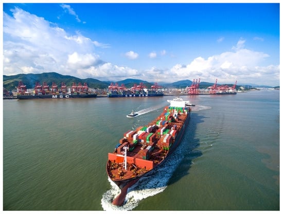
Figure 1.
Zhoushan Port during operation.
The paper is organized as follows: Section 2 introduces the study area and instruments, data and methods, and the division method for each stage of the sea fog process. Section 3 introduces the evolution of macroscopic and microscopic characteristics over time and the correlation between microphysical properties. Section 4 presents the conclusion and discussion.
2. Data and Methods
2.1. Study Area
The core port area of Ningbo Zhoushan Port is located between the Beilun District of Ningbo City and the Dinghai District of Zhoushan City, and it is a long and narrow area from east to west. In 2021, the Key Laboratory of Atmospheric Sounding of the China Meteorological Administration (KLAS, Chengdu, China) and the Ningbo Meteorological Network and Equipment Support Center (NBMSC, Ningbo, China) jointly carried out a sea fog monitoring experiment in Meishan Port District, Beilun District. A distribution map of the sea fog observation equipment, namely, the visibility meter (29.78°N, 121.88°E), the fog monitor (29.74°N, 121.9°E), and the automatic weather station (29.76°N, 121.9°E), is shown in Figure 2.
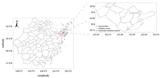
Figure 2.
Distribution map of instruments and the automatic weather station. The map on the left is Zhejiang Province, China. The pink part is the Beilun District.
2.2. Data and Methods
The data used in this paper comprise the observation data of the visibility meter, the automatic weather station, and the fog monitor (Table 1). Among them, the CJY-1G forward visibility scatterometer produced by Luoyang Kaimai Company (Luoyang, China) is a new generation of intelligent atmospheric visibility monitoring equipment with a simple structure, low power consumption, and strong reliability, and it can obtain visibility (V) data. As a ground meteorological automatic observation system, the DZZ4 automatic weather station produced by Aerospace New Weather Technology Co., Ltd. (Wuxi, China) can collect data on temperature (T), relative humidity (RH), wind speed (WS), and other elements. The FM-120 fog monitor is an optical instrument manufactured by DMT to measure the particle size distribution of clouds and fog using laser forward scattering technology (Figure 3). It can be installed on the ground or on tower buildings to study fog conditions. The instrument uses a solid-state laser diode as the core component, and its surface is integrated with electronic technology. The fog monitor can be applied to harsh environments and operates in a stable and reliable manner. It can realize the continuous observation of the microphysical data of cloud and fog processes. The diameter of the observed particles (cloud (fog) droplets) ranges from (D) 2 to 50 μm, the sampling area is 0.24 mm2, the frequency is 1 s−1, and the speed of the exhaust port is about 15 m s−1. The observed physical quantities mainly include the droplet number concentration (Nc), particle number content of different diameters (n(D)), liquid water content (LWC), equivalent diameter (ED), and median volume diameter (MVD).

Table 1.
Observation equipment and related technical parameters.
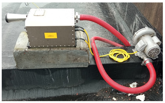
Figure 3.
The actual installation of the FM-120 fog monitor.
Using the observation data of the fog monitor, we established a quantitative calculation index for the microphysical characteristics of sea fog (Table 2). Among them, r is the droplet radius; D is the droplet diameter; and N0, μ, and λ are the three parameters in the curve.
Table 2.
Calculation formulas of physical quantities used in the subsequent analysis.
In order to analyze the characteristics of the different stages of the entire sea fog process, we divided the generation and elimination stages in this study according to the change laws of V, NC, LWC, and as follows [23]: (1) Gestation stage: during this stage, visibility changes significantly, and NC and LWC increase from about 0; (2) Formation stage: during this stage, visibility drops below 1 km, and the growth rates of the other three characteristic parameters, such as, NC are low; (3) Development stage: during this stage, visibility continues to decrease, and the other characteristic parameters significantly increase; (4) Maturation stage: during this stage, visibility is maintained at a low value, and each characteristic parameter reaches its maximum value; (5) Intermittent stage: during this period, visibility increases to more than 1 km, and each characteristic parameter remains at a low value; and (6) Dissipation stage: during this stage, visibility increases, and each characteristic parameter decreases.
3. Results and Analysis
3.1. Overview of the Sea Fog
In Figure 4, we can see the evolution characteristics of visibility (V), temperature (T), wind speed (WS), and relative humidity (RH) over time during the sea fog process. Due to differences in time resolution, the visibility data were averaged every 5 min. It can be seen that the entire sea fog process lasted for about 9 h, and the lowest visibility was less than 200 m. The sea fog began to form at 23:00 (LT) on 14 June and dissipated at 7:20 (LT) on 15 June. Figure 5 shows a real-time photograph of the sea fog at the port at 6:03 (LT) on 15 June 2021. The temperature varied in the range of 23 to 26 °C. It decreased slightly at 0:30 (LT) on the 15th, and the visibility gradually increased as the temperature increased after 5:40 (LT). The relative humidity was always higher than 98%, and the near-saturated state promoted the formation of fog droplets. Visibility, temperature, and wind speed all show a trend of first oscillating down and then oscillating up; that is, they roughly have the same trend. In the whole sea fog process, the wind speed did not exceed 2 m/s, and the fluctuation in the ground wind speed was not obvious, indicating that advection had little effect on the change in the microphysical structure during the fog process and that the change in the microphysical structure was mainly related to the microphysical process that occurs in the fog [24]. Therefore, the microphysical characteristics of this process were analyzed below.
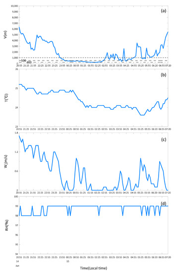
Figure 4.
Example of the evolution of meteorological elements. The example time is 20:55 on 14 June to 7:20 on 15 June. (a) V, (b) T, (c) WS, (d) RH. The dotted lines represent 1000 m, 500 m, and 200 m (Figure 4a).
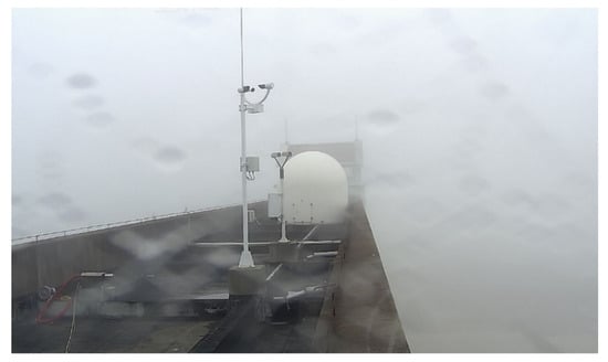
Figure 5.
A real-time photograph of sea fog at 6:03 (LT) on 15 June 2021 at the port where the droplet spectrometer is located. The lower left corner of the photograph is the fog monitor (FM-120).
3.2. Microphysical Features
3.2.1. Features of Each Stage
From the change in visibility (Figure 6), we can see that the entire sea fog presents two types of change trends. For the convenience of analysis, we divide these into two processes: case1 and case2. According to the method proposed in Section 2.2, case1 occurs from 14 June 23:31 to 15 June 2:59, and case2 occurs from 15 June 3:46 to 15 June 7:20 (Table 3). Figure 6 shows the evolution characteristics of V, NC, LWC, , and CV over time during this sea fog process. Due to differences in time resolution, NC, LWC, and are averaged every minute. It can be seen that the microphysical structure changes significantly during the whole process, and V and microphysical quantities, such as NC, show roughly opposite trends.
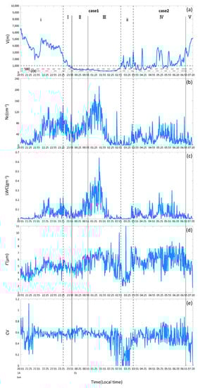
Figure 6.
Example of the evolution of microphysical quantities. The example time is 20:55 on 14 June to 7:20 on 15 June. (a) V, (b) NC, (c) LWC, (d) , (e) CV. The lines in the figure represent the divisions of the stages.
Table 3.
Subdivide the stage of sea fog from 20:55 on 14 June to 7:20 on 15 June.
According to the change characteristics of the physical quantities at different development stages in the entire sea fog process, we can preliminarily determine the following:
In the formation stage of the case1 process, NC, LWC, , and CV show a small oscillating change, indicating that collision and coalescence at this stage are very weak. In the development stage of the case1 process, NC, LWC, and all show a relatively consistent increase trend, and CV shows an oscillating change characteristic, indicating that a large number of condensation nuclei form new droplets through nucleation and condensation growth in this stage. With an increase in the number concentration, the continuous collision growth process starts, large droplets collide with small droplets, and the average radius increases. The finding of NC increasing at this stage rather than decreasing is different from the phenomenon summarized by Liu et al., who stated that collision–coagulation leads to an increase in large droplets and a decrease in tiny droplets [25]. In the maturation and dissipation stages of the case1 process, V decreases to less than 200 m. NC, LWC, and continue to increase during the initial stage and then decrease, and NC and LWC reach their maximum values for the whole process. CV fluctuates during the initial stage and decreases at a later stage. The above shows that continuous collision and growth processes still occur in the early stages and that the processes then weaken. During the formation and development stages of the case2 process, V greatly fluctuates, during which three brief dense fog processes occur. A larger indicates that an inevitable collision process occurs [26].
Temperature is closely related to nucleation, condensation growth, and other processes. A temperature drop (increase) is the main reason for nucleation enhancement (weakening) and condensation growth (droplet evaporation), which leads to an increase (or decrease) in microphysical quantities, such as number concentration and liquid water content.
In Figure 6, we can see that the visibility of the case1 process remains at a low value for a long time. To more intuitively understand the specific conditions of the microphysical feature quantities at the different stages of the process, we count NC, LWC, and of the case1 process, gestation stage, and intermittent stage (Table 4). It can be seen that there are significant differences in the microphysical parameters at the different stages of the sea fog.
Table 4.
Average, maximum, and minimum values of key characteristic parameters of case1 process, gestation stage, and intermittent stage.
In addition, regarding the change over time in the number concentration of particles with different diameters (Figure 7), when the visibility significantly decreased, the number of particles in each interval dramatically increased, and the droplet spectrum dramatically expanded, but the increased range was different. The number of particles with diameters of 3.5~6.5 μm and 14~26 μm significantly increased the most, and the maximum number was more than 58 cm−3. A further analysis of Figure 7 shows that the number of particles larger than 11 μm continued to increase, even more so than small particles (from 1:01 to 1:45). This is because the water vapor is sufficient at this stage, condensation nucleation and condensation growth vigorously develop, and collision and coalescence continue to occur. In summary, the high concentration of small droplets indicates that many condensation nuclei are nucleated and that the water vapor condenses on the smaller condensation nuclei and rapidly grows [27]. The high concentration of large particles indicates that the collision effect is strong and that the small particles aggregate into large particles. The co-increase of large particles and small particles leads to an increase in the particle number concentration.
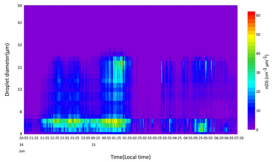
Figure 7.
Change in particle number concentration (color-filled) with different diameters over time from 20:55 on 14 June to 7:20 on 15 June 2021.
3.2.2. Features of the Droplet Spectrum
The spectral distribution of fog droplets is another critical parameter that reflects the microphysical characteristics of fog. To study the differences in the microphysical characteristics of case1 and case2 of the sea fog process in Beilun District, Figure 8 shows the droplet spectrum distribution at each stage of the sea fog process in Beilun District from 14 to 15 June 2021. The logarithmic coordinate is used as the ordinate to better reflect the difference in the spectral width of droplets and the density of large droplets at each stage [28]. The high value of the number concentration at each stage is concentrated in the small droplets (diameter between 4 and 6 μm), the droplet spectrum is relatively broad, and the maximum diameter is close to 50 μm, but the number concentration is minimal. Among them, the maximum number concentration of droplets with a diameter of 8–12 μm is observed in the formation stage of case1 (I), the maximum number concentration of droplets with a diameter of 15–27 μm is observed in the maturation stage of case1 (III), and the maximum number of droplets with a diameter of 36–47 μm is observed in the developmental stage of case1 (II).
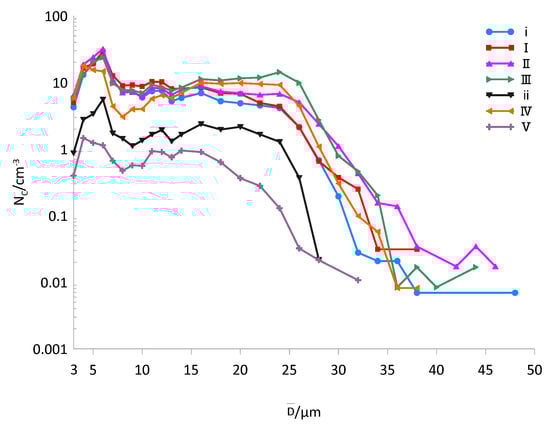
Figure 8.
Droplet spectrum distribution at each stage of sea fog process in Beilun district from 20:55 on 14 June to 7:20 on 15 June 2021.
In the study of the microphysical laws of cloud, fog, and precipitation, almost all the problems involve particle scale, which is the most fundamental parameter. The particle swarm is of practical significance, and it is a combination of particle size and number concentration. The droplet spectral distribution function needs to be represented, and the Gamma function can be used to describe it [29,30,31]. In practical applications and theoretical research, using the Gamma function to replace the exponential spectrum in order to approximate the actual spectrum is mainly carried out by employing the direct observation method, which is rarely verified in mathematics. Liu introduced two statistical parameters, skewness (Sk) and kurtosis (Ku), to analyze the actual distribution characteristics of droplet spectra and applied them to a fitting analysis of the droplet spectrum type. When Sk = Ku = 0, the spectrum has a normal distribution; when Sk > 0, it has a positive skewed distribution; when Sk < 0, it has a negative skewed distribution; when Ku > 0, the spectra is leptokurtic; when Ku < 0, the spectra is platykurtic. We introduce CS (skewness deviation coefficient) and Ck (kurtosis deviation coefficient), which give an indication of the deviation of skewness and kurtosis from their values for the M-P distributions [32,33]. Assuming that the particle spectral distribution satisfies the Gamma function, CS = Ck, and we can verify whether the spectral distribution satisfies the Gamma distribution by calculating the CS = Ck of the actual spectrum. Now, we use the data from this sea fog process to calculate CS = Ck and to draw a scatter plot (Figure 9). It can be seen in the figure that most of the scatter points are near the straight line y = x, indicating that the droplet spectrum distribution roughly conforms to the Gamma distribution. Comparing the droplet spectrum distributions of the sea fog between different regions, it is obvious that they are different from the monotonically decreasing types in Zhanjiang, Maoming, and Qingdao. Among them, the droplet spectra in Zhanjiang and Maoming conform to the Junge distribution [34,35], and the droplet spectra in the coastal areas of Zhoushan and southern Fujian conform to the Deirmenjian distribution [36,37]. However, the spectral droplet distribution of the sea fog process in Zhanjiang from 20 to 21 March 2011 satisfies the Gamma distribution [38].
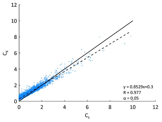
Figure 9.
Kurtosis deviation coefficient (Ck) is a function of the skewness deviation coefficient (CS). The solid line is Y = X, and the dotted line represents the regression line of the whole fog event.
Figure 10 shows the average droplet spectrum of this sea fog process. As can be seen in Figure 8 and Figure 10, the spectral distribution of the fog process presents a “multi-peak” structure, with peak diameters of 6 μm, 12 μm, 16 μm, 24 μm, and 44 μm. The proportion of droplets with a diameter of less than 16 μm is 75%. It can be seen in Figure 7 that the number concentration of particles with diameters of 6μm and 22–24 μm is the largest. Therefore, we fit the average spectrum into two sections according to the measured data and the Gamma distribution.
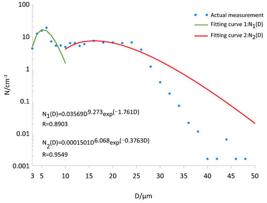
Figure 10.
The average spectral distribution of sea fog process in Beilun district from 20:55 on 14 June to 7:20 on 15 June 2021.
3.2.3. Features of Correlation and Difference
The relationships with crucial microphysical factors are discussed to further understand the main microphysical processes affecting sea fog. A scatter diagram of the three microphysical parameters is drawn for the correlation analysis (Figure 11). Figure 11a shows the relationship between NC and mean diameter () during the entire sea fog process, and R is the correlation coefficient. The positive correlation between NC and of the whole process is weak (R = 0.3092). NC and LWC in Figure 11b have an excellent positive correlation (R = 0.8922). in Figure 11c also has an excellent positive correlation with LWC. Many previous cloud theories state that the growth of clouds is achieved by the activation of small particles, the further enlargement of droplets, and the collection effect after condensation [39]. The collision process causes droplets to collide and combine, and the diameter increases while the number concentration reduces, breaking the positive correlation trend between the number concentration and the average diameter. The three microphysical parameters in the figure are all positively correlated, but the positive correlation between NC and is weak. We can conclude that this sea fog process is dominated by condensation nucleation and the condensation growth of droplets [40] and that the collision process occurs, but it is not the dominant process, which is consistent with the previous analysis.
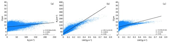
Figure 11.
The correlation analysis of the two parameters in the Beilun district from 20:55 on 14 June to 7:20 on 15 June 2021. (a) (μm) and NC (cm−3), (b) NC (cm−3) and LWC (g m−3), (c) (μm) and LWC (g m−3).
There are differences in the microphysical characteristics at different stages of the sea fog process. We analyzed the correlation between NC and in the case1 process, gestation stage, and intermittent stage (Figure 12). From the gestation stage to the development stage, the correlation decreases, indicating that collision and coalescence gradually strengthen. At the maturation and dissipation stages, the correlation becomes larger, but this does not mean that the collision effect at this stage is weakening. It can be seen in Figure 6c that water vapor is particularly sufficient in the early stage of this process, so the condensation nuclei are continuously activated, while the droplets condense and grow. The continuous regeneration of small droplets consolidates the increase in the number concentration; thus, the correlation becomes larger. The correlation coefficient of the intermittent period continues to increase, and the collision process weakens at this stage.
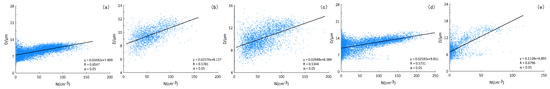
Figure 12.
Correlation analysis between (μm) and NC (cm−3) in the case1 process, gestation stage, and intermittent stage. (a) Gestation stage, (b) formation stage, (c) development stage, (d) maturation and dissipation stage, (e) intermittent stage.
The generation and disappearance of fog are complex processes, and not only are they related to the weather situation, but they are also related to the local climate background, geographical environment, and aerosol distribution characteristics. Therefore, fog processes across different regions, or even in the same region, often have different microphysical quantities. At the same time, microphysical parameters can quantitatively describe the microphysical characteristics of sea fog [41]. Table 5 compares the average values and variation ranges of microphysical quantities between sea fog cases in the Beilun District, China, and other coastal areas to understand the characteristics of sea fog in the study area. It is found that the average values of LWC in each area have little difference, but the maximum value in the Beilun area is larger than that in the other areas, indicating that water vapor in the Beilun area is more abundant. The of fog in Zhoushan is relatively large, followed by that in the Beilun area. Different observation instruments may have caused this particular result. The particle size measurement range of the three-purpose droplet spectrometer is 3.2–70 μm, while the range of the laser backscattering droplet spectrometer is 2–50 μm. NC in the Beilun area is low, which is related to the large average radius of fog droplets. The microphysical characteristics of Beilun District are analyzed in depth below.
Table 5.
Comparison of individual cases of sea fog microphysical characteristics between the Beilun District of Ningbo City and other coastal areas in China.
4. Discussion
This study fills the gap in sea fog microphysics research in the Meishan Port area of the Beilun District. This shows that, as expected, the condensation nucleation and the condensation growth of droplets are the main processes in this sea fog process and that the collision process occurs but is not the dominant process. The high concentration of small droplets indicates that many condensation nuclei are nucleated, and the water vapor condenses on the smaller condensation nuclei and grows rapidly. The collision process causes the droplets to collide and combine, and the diameter increases while the number concentration reduces, breaking the positive correlation trend between the number concentration and the average diameter.
5. Conclusions
This paper uses the observation data of a fog monitor, a visibility meter, and an automatic weather station to analyze the sea fog process in Beilun District, China, from 14 to 15 June 2021. We discuss the evolution of the macroscopic and microscopic characteristics of the sea fog process and the correlation between microphysical properties and their effects on visibility. The main conclusions are as follows:
- During the whole sea fog process, visibility has roughly the same change trend as temperature and wind speed, and it shows roughly an opposite change trend to microphysical quantities, such as number concentration and liquid water content.
- The change in the microphysical structure is mainly related to the microphysical process of fog, and the advection has little effect on the change in the microphysical structure. Temperature is closely related to nucleation, condensation growth, and other processes. The decrease (increase) in temperature is the main reason for the enhancement (weakening) of nucleation and the growth of condensation (evaporation of droplets), which leads to an increase (or decrease) in microphysical quantities, such as the droplet number concentration and liquid water content.
- The average droplet spectral distribution roughly conforms to the Gamma distribution, and the spectral distribution of the fog process presents a “multi-peak” structure, with peak diameters of 6 μm, 12 μm, 16 μm, 24 μm, and 44 μm. A large proportion of droplets have a diameter of less than 16 μm, accounting for 75%. Comparing the droplet spectrum distributions of sea fog between different regions, the droplet spectra in Zhanjiang and Maoming conform to the Junge distribution, and in the droplet spectra in the coastal areas of Zhoushan and southern Fujian conform to the Deirmenjian distribution. However, the spectral droplet distribution of the sea fog process in Zhanjiang from 20 to 21 March 2011 satisfies the Gamma distribution.
- During this sea fog process, three microphysical parameters, namely, number concentration, liquid water content, and average diameter, are all positively correlated in pairs, but the positive correlation between number concentration and average diameter is weak. This sea fog process is dominated by condensation nucleation and the condensation growth of droplets. The collision process mainly occurs in the development and maturation stage of the case1 process and the formation and development stages of the case2 process, and it is weak in other stages. The number concentration in the development and maturation stage of case1 increases rather than decreases, which may be due to the sufficient water vapor at this stage; the development of condensation nucleation and condensation growth is robust; collision and coalescence continue to occur; small particles aggregate into large particles; and the number of large particles increases. At the same time, condensation and nucleation ensure the stability of the number concentration of small particles.
This study provides a more in-depth analysis of sea fog’s generation and dissipation mechanisms, primarily providing more reference information for sea fog research and equipment comparisons between different regions. However, due to limited observation data, more observations are needed to verify the above conclusions in the future. In addition, during this sea fog process, aerosols may affect microphysical parameters, such as number concentration and liquid water content, but we do not discuss them here. To further study the above issues, we will continue to conduct observations on offshore observation platforms, increase monitoring means, and strengthen monitoring capabilities [44,45]. In addition, we will carry out more research on numerical simulations of sea fog, conduct a more in-depth analysis of the evolution and causes of sea fog microphysical processes, and verify the observation results to provide a microphysical basis for the short-term forecast of sea fog, the optimization of the microphysical parameters of related models, and more reference information for sea fog research and equipment comparisons between different regions.
Author Contributions
Conceptualization, J.H., X.R., H.W. and Z.S.; methodology, J.H., X.R. and F.Z.; software, J.H., X.R. and Q.Z.; formal analysis, J.H., X.R. and X.J.; writing—original draft preparation, X.R.; writing—review and editing, J.H., X.R. and H.W.; visualization, J.H., X.R. and L.H. All authors have read and agreed to the published version of the manuscript.
Funding
This work was supported by the National Key R&D Program of China (2021YFC3090203), a Project of the Sichuan Department of Science and Technology (2022YFS0541), the Key R&D Program of Yunnan Provincial Department of Science and Technology (202203AC100006), and the Key Laboratory of Atmospheric Sounding Program of China Meteorological Administration (2021KLAS02Z).
Data Availability Statement
Not applicable.
Acknowledgments
The authors would like to express their sincere thanks to Ningbo Meteorological Network and Equipment Support Center for supplying the data used in this manuscript and the reviewers for their constructive comments and editorial suggestions that considerably helped improve the quality of the manuscript.
Conflicts of Interest
The authors declare no conflict of interest.
References
- Gultepe, I.; Milbrandt, J.A. Microphysical observations and mesoscale model simulation of a warm fog case during FRAM project. In Fog and Boundary Layer Clouds: Fog Visibility and Forecasting; Birkhäuser: Basel, Switzerland, 2007; pp. 1161–1178. [Google Scholar]
- Zhang, S.; Ren, Z.; Liu, J.; Yang, Y.; Wang, X. Variations in the lower level of the PBL associated with the Yellow Sea fog-new observations by L-band radar. J. Ocean Univ. China 2008, 7, 353–361. [Google Scholar] [CrossRef]
- Lee, H.Y.; Chang, E.C. Impact of land-sea thermal contrast on the inland penetration of sea fog over the coastal area around the Korean Peninsula. J. Geophys. Res. Atmos. 2018, 123, 6487–6504. [Google Scholar] [CrossRef]
- The British Maritime Coast Guard Agency. Navigation in Restricted Visibility. Pilot NoticeMGN 369. 2008. Available online: https://assets.publishing.service.gov.uk/government/uploads/system/uploads/attachment_data/file/855852/MGN_369.pdf (accessed on 4 September 2022).
- Auckland Regional Council. Harbourmaster Periods of Restricted Visibility; Auckland Regional Council: Auckland, New Zealand, 2011. [Google Scholar]
- Bundes Ministerium for Verkehr Baus Office. Operation of Vessels during and Statent Wicklung. German Traffic Regulations for Navigable Maritime Waterways; Bundes Ministerium for Verkehr Baus Office: Berlin, Germany, 2012. [Google Scholar]
- Leigh, R.J. Economic benefits of terminal aerodrome forecasts (TAFs) for Sydney airport, Australia. Meteorol. Appl. 1995, 2, 239–247. [Google Scholar] [CrossRef]
- Pilié, R.J.; Mack, E.J.; Rogers, C.W.; Katz, U.; Kocmond, W.C. The formation of marine fog and the development of fog-stratus systems along the California coast. J. Appl. Meteorol. Climatol. 1979, 18, 1275–1286. [Google Scholar] [CrossRef]
- Findlater, J.; Roach, W.T.; McHugh, B.C. The haar of north-east Scotland. QJR Meteorol. Soc. 1989, 115, 581–608. [Google Scholar] [CrossRef]
- Gultepe, I.; Pearson, G.; Milbrandt, J.A.; Hansen, B.; Platnick, S.; Taylor, P.; Gordon, M.; Oakley, J.P.; Cober, S.G. The fog remote sensing and modeling field project. Bull. Am. Meteorol. Soc. 2009, 90, 341–360. [Google Scholar] [CrossRef]
- Isaac, G.A.; Bullock, T.; Beale, J.; Beale, S. Characterizing and predicting marine fog offshore Newfoundland and Labrador. Weather Forecast 2020, 35, 347–365. [Google Scholar] [CrossRef]
- Fernando, H.J.; Gultepe, I.; Dorman, C.; Pardyjak, E.; Wang, Q.; Hoch, S.W.; Richter, D.; Creegan, E.; Gaberšek, S.; Bullock, T.; et al. C-FOG: Life of coastal fog. Bull. Am. Meteorol. Soc. 2021, 102, 244–272. [Google Scholar] [CrossRef]
- Niu, S.; Lu, C.; Yu, H.; Zhao, L.; Lü, J. Fog research in China: An overview. Adv. Atmos. Sci. 2010, 27, 639–662. [Google Scholar] [CrossRef]
- Eldridge, R.G. The relationship between visibility and liquid water content in fog. J. Atmos. Sci. 1971, 28, 1183–1186. [Google Scholar] [CrossRef]
- Meyer, M.B.; Jiusto, J.E.; Lala, G.G. Measurements of visual range and radiation-fog (haze) microphysics. J. Atmos. Sci. 1980, 37, 622–629. [Google Scholar] [CrossRef]
- Kunkel, B.A. Parameterization of droplet terminal velocity and extinction coefficient in fog models. J. Appl. Meteorol. Climatol. 1984, 23, 34–41. [Google Scholar] [CrossRef]
- Goodman, J. The microstructure of California coastal fog and stratus. J. Appl. Meteorol. Climatol. 1977, 16, 1056–1067. [Google Scholar] [CrossRef]
- Bott, A.; Sievers, U.; Zdunkowski, W. A radiation fog model with a detailed treatment of the interaction between radiative transfer and fog microphysics. J. Atmos. Sci. 1990, 47, 2153–2166. [Google Scholar] [CrossRef]
- Zhao, L.; Niu, S.; Zhang, Y.; Xu, F. Microphysical characteristics of sea fog over the east coast of Leizhou Peninsula, China. Adv. Atmos. Sci. 2013, 30, 1154–1172. [Google Scholar] [CrossRef]
- Gultepe, I.; Tardif, R.; Michaelides, S.C.; Cermak, J.; Bott, A.; Bendix, J.; Müller, M.D.; Pagowski, M.; Hansen, B.; Ellrod, G.; et al. Fog research: A review of past achievements and future perspectives. Pure Appl. Geophys. 2007, 164, 1121–1159. [Google Scholar] [CrossRef]
- Liu, D.; Li, Z.; Yan, W.; Li, Y. Advances in fog microphysics research in China. Asia Pac. J. Atmos. Sci. 2017, 53, 131–148. [Google Scholar] [CrossRef]
- Gultepe, I.; Milbrandt, J.A.; Zhou, B. Marine fog: A review on microphysics and visibility prediction. In Marine Fog: Challenges and Advancements in Observations, Modeling, and Forecasting; Koracin, D., Dorman, C., Eds.; Springer: Berlin/Heidelberg, Germany, 2017; pp. 345–394. [Google Scholar]
- Zhang, Y.; Fan, S.X.; Zhang, S.T.; Wei, J.C. Microstructures and temporal variation characteristics during a sea fog event along the west coast of the Taiwan Strait. J. Trop. Meteorol. 2017, 23, 155–165. [Google Scholar]
- Li, Z.; Liu, D.; Yan, W.; Wang, H.; Zhu, C.; Zhu, Y.; Zu, F. Dense fog burst reinforcement over Eastern China: A review. Atmos. Res. 2019, 230, 104639. [Google Scholar] [CrossRef]
- Liu, D.; Yang, J.; Niu, S.; Li, Z. On the evolution and structure of a radiation fog event in Nanjing. Adv. Atmos. Sci. 2011, 28, 223–237. [Google Scholar] [CrossRef]
- Liu, Q.; Wu, B.; Wang, Z.; Hao, T. Fog droplet size distribution and the interaction between fog droplets and fine particles during dense fog in Tianjin, China. Atmosphere 2020, 11, 258. [Google Scholar] [CrossRef]
- Wang, S.; Yi, L.; Zhang, S.; Shi, X.; Chen, X. The microphysical properties of a sea-fog event along the west coast of the yellow sea in spring. Atmosphere 2020, 11, 413. [Google Scholar] [CrossRef]
- Liu, D.; Pu, M.; Yang, J.; Zhang, G.; Yan, W.; Li, Z. Microphysical structure and evolution of a four-day persistent fog event in Nanjing in December 2006. Acta Meteorol. Sin. 2010, 24, 104–115. [Google Scholar]
- Hsieh, W.C.; Jonsson, H.; Wang, L.P.; Buzorius, G.; Flagan, R.C.; Seinfeld, J.H.; Nenes, A. On the representation of droplet coalescence and autoconversion: Evaluation using ambient cloud droplet size distributions. J. Geophys. Res. Atmos. 2009, 114, D7. [Google Scholar] [CrossRef]
- Costa, A.A.; de Oliveira, C.J.; de Oliveira, J.C.P.; da Costa Sampaio, A.J. Microphysical observations of warm cumulus clouds in Ceara, Brazil. Atmos. Res. 2000, 54, 167–199. [Google Scholar] [CrossRef]
- Schmitt, C.G.; Stuefer, M.; Heymsfield, A.J.; Kim, C.K. The microphysical properties of ice fog measured in urban environments of Interior Alaska. J. Geophys. Res. Atmos. 2013, 118, 11–136. [Google Scholar] [CrossRef]
- Liu, Y. Skewness and kurtosis of measured raindrop size distributions. Atmos. Environ. 1992, 26, 2713–2716. [Google Scholar]
- Liu, Y. Statistical theory of the Marshall-Palmer distribution of raindrops. Atmos. Environ. 1993, 27, 15–19. [Google Scholar]
- Huang, H.; Huang, J.; Liu, C.; Yuan, J.; Lü, W.; Yang, Y.; Liao, F. Microphysical structural characteristics of sea fog in Maoming. Haiyang Xuebao 2009, 2, 17–23. (In Chinese) [Google Scholar]
- Zhang, S.; Niu, S.; Zhao, L. A case analysis of the microphysical structure of sea fog in the South China Sea. Chin. J. Atmos. Sci. 2013, 27, 552–562. (In Chinese) [Google Scholar]
- Yang, Z.; Xu, S.; Geng, P. Formation and microphysical structure of spring sea fog in Zhoushan area. Haiyang Xuebao 1989, 11, 431–438. (In Chinese) [Google Scholar]
- Zhang, W.; Chen, D.; Hu, Y.; Xun, A.; Jiang, Y.; Sun, X. Microphysical characteristics analysis of a spring sea fog process along the coast of southern Fujian. Meteor Mon. 2021, 47, 157–169. (In Chinese) [Google Scholar]
- Yue, Y.; Niu, S.; Zhao, L.; Zhang, Y.; Xu, F. Analysis of weather conditions and macro and micro characteristics of coastal fog in Zhanjiang area. Chin. J. Atmos. Sci. 2013, 27, 609–622. (In Chinese) [Google Scholar]
- Podzimek, J. Droplet concentration and size distribution in haze and fog. Studia Geophys. Geod. 1997, 41, 277–296. [Google Scholar] [CrossRef]
- Niu, S.; Lu, C.; Liu, Y.; Zhao, L.; Lü, J.; Yang, J. Analysis of the microphysical structure of heavy fog using a droplet spectrometer: A case study. Adv. Atmos. Sci. 2010, 27, 1259–1275. [Google Scholar] [CrossRef]
- Zhang, J.; Xue, H.; Deng, Z.; Ma, N.; Zhao, C.; Zhang, Q. A comparison of the parameterization schemes of fog visibility using the in-situ measurements in the North China Plain. Atmos. Environ. 2014, 92, 44–50. [Google Scholar] [CrossRef]
- Huang, H.; Huang, J.; Mao, W.; Liao, F.; Li, X.; Lü, W.; Yang, Y. Evolution characteristics of water content in sea fog and its relationship with atmospheric horizontal visibility in Maoming area. Haiyang Xuebao 2010, 32, 40–53. (In Chinese) [Google Scholar]
- Xu, F.; Han, L.; Lü, J.; Wang, J.; Tu, S.; Ji, Q.; Zhang, Y. Microphysical and chemical characteristics of a sea fog in the northwestern South China Sea. Chin. J. Trop. Meteorol. 2019, 35, 596–603. (In Chinese) [Google Scholar]
- Hu, L.; Yang, H.; Wang, H.; Ren, X. Joint Monitoring and Analysis of Sea Fog Using Dual Visibility Lidar in Ningbo, China. In Journal of Physics: Conference Series; IOP Publishing: Bristol, UK, 2021; Volume 2112, p. 012014. [Google Scholar]
- Hu, L.; Yang, H. Monitoring and analysis of sea fog in an offshore waterway using lidar. Opt. Eng. 2021, 60, 064103. [Google Scholar] [CrossRef]


Publisher’s Note: MDPI stays neutral with regard to jurisdictional claims in published maps and institutional affiliations. |
© 2022 by the authors. Licensee MDPI, Basel, Switzerland. This article is an open access article distributed under the terms and conditions of the Creative Commons Attribution (CC BY) license (https://creativecommons.org/licenses/by/4.0/).