Abstract
We present new advances in monitoring particulate matter (PM) in urban areas within a participatory vehicle sensor network (VSN) that exploits the use of multiple mobile low-cost IoT devices. These devices send geolocated PM measurements to an IT infrastructure and enabled us to reconstruct, in real time, the spatial and temporal distribution of pollutants in the study area in a web-based environment. The newly acquired data were integrated with independent reference measurements available from governmental environmental agencies. We deployed the infrastructure in the city of Trieste (Italy), since the beginning of 2021, with the help of several volunteers and the local transportation authority (Trieste Trasporti). By analysing the data, we delineate areas with lower air quality and identify the possible causes of these anomalies. We were able to define a belt outside the urban center where an enhanced concentration of pollutants occurs due to a higher flux of vehicular traffic that tends to jam there. Overall, our results demonstrate that this approach can be helpful in supporting urban planning and can also stimulate the community to reflect on how they can improve air quality in the area they live by reducing the use of private cars in favour of more widespread public transportation usage.
1. Introduction
Air pollution is the contamination of the environment by chemical, physical, or biological agents that modify the natural characteristics of the atmosphere.
Respiratory diseases, including asthma and chronic obstructive pulmonary disease, are responsible for approximately 10% of non-communicable diseases deaths [1]. Exposure to air pollution may increase the risk of pulmonary infection [2]. This is particularly evident for long-term exposure to particulate matter (PM) and nitrogen dioxide (NO2) [3,4], while concerns have been highlighted by several authors regarding the possible correlation between COVID-19 occurrence and air quality [5].
Air pollutants are commonly differentiated as outdoor or indoor. Outdoor pollutants are caused by fossil fuel or biomass combustion, automobile exhaust fumes, wind-blown dust, and industry and construction emissions. Indoor pollutants are released while cooking or heating, from cigarette smoke, or household cleaning. Sources of air pollution are not homogeneously distributed geographically. Some authors report on differences between low-income and high-income countries and between urban and rural areas [6].
Natural factors, such as topography, meteorological conditions, and land cover type exert great influence over the processes of diffusion and elimination of air pollutants [7]. Megaritis et al. [8], for example, highlight the influence of temperature on the secondary products of particulate matter, while Alvarez et al. [9] correlate particulate matter concentrations with topography. The concentration of air pollutants can therefore be highly dependent on the specific setting of the designated area, so that, where natural factors show significant gradients, high resolution studies are needed to better understand and model phenomena [10].
PM is a mixture of organic and inorganic solid particles and liquid droplets suspended in air that is classified based upon the size of its particles. Larger particles with a size less than 10 µm are classified as PM10, smaller particles with a size up to 2.5 µm are classified as PM2.5, while the ultrafine fraction contains particles smaller than 0.1 µm.
The classification of PM based upon its diameter is based on its aerodynamic properties. This is because aerodynamic properties control the transport and removal of particles from the air and, importantly, they also control the deposition of PM within the human respiratory system [11]. Significant studies exist on the effects of PM on health, such as [12], which asserts that the risk of cardiopulmonary mortality is already elevated at PM2.5 levels of 10 µg/m3. Larger PM particles contain dust from roads and industries, while the fine particles are primarily produced during biomass and fossil fuel combustion [11,12].
Air quality is generally assessed by governmental environmental agencies through ground-based monitoring stations that use high accuracy and precision devices that are deployed in a network of fixed positions. These stations are generally sparse because the costs of instrumentation and logistics are very high. Uncovered areas and regional scenarios are estimated using statistical interpolation methods [13] and/or modelling [14].
In highly dynamic environments this can be problematic. At the end of 1990, Irwin [15] introduced, in scientific research, a new approach based on the possibility of enrolling volunteers with no specific scientific competence. Following [16], this new approach is particularly suitable for data acquisition activities. With slight differences, this new paradigm can be declined as citizen science or crowdsensing [17]. Citizen science refers to the case where laypeople are involved in research activities while being enabled to build their knowledge on a specific scientific topic. Crowdsensing, instead, focusses on the opportunistic use of volunteers as acquisition platforms. Volunteers can be private citizens, but also larger communities, and in this sense crowdsensing can also be based on the help of private or public companies interested in contributing to scientific research.
Opening science to the contribution of the society at large is extremely important since this allows one to contrast ‘fake news’ that very easily and quickly circulates in social media [18,19]. Citizen science and crowdsensing have been progressively used in more and more scientific fields, such as archeology [20], epidemiology [21], and the environmental sciences [22]. The crowdsensing approach has also been adopted by our team in previous projects devoted to monitoring the environment [19,23,24,25].
This paper focuses on the application of the crowdsensing paradigm to real-time monitoring of PM concentrations using mobile acquisition platforms in order to identify areas with lower air quality and figure out possible causes of these anomalies.
Related Work
The recent introduction of low-cost sensors (LCS) has expanded the possibilities for air quality monitoring. LCSs allow one to gather high-resolution spatial and temporal data from numerous individual nodes, which allows for better interpolation of sparse data and the generation of denser maps of air quality. These denser geographic distributions can become very good estimates of real-life pollution–dispersion scenarios [26]. LCSs are based on optical particles counters (OPCs) [27] and solid-state sensors [28]. LCS technologies for air quality monitoring advanced quickly, producing an already significant literature [29,30,31,32]. At the same time, the availability of LCSs has enabled a large number of participatory monitoring initiatives such as Sensor.Community [33] and Airflux [34]. These initiatives will increasingly involve citizens in the activity of collecting data on air pollution while allowing them to develop a correct view on the environmental phenomena that surround them. The environmental awareness resulting from citizens’ participative research will allow them to take an active part into tackling issues such as urban traffic or house heating emissions.
Following [35], participatory air quality monitoring initiatives can be divided into three main categories, namely: the (i) static sensor network (SSN); the (ii) community sensor network (CSN); and the (iii) vehicle sensor network (VSN). SSN is the case where wireless sensors are deployed at fixed positions. Examples of this type of deployment are [36] or [37]. CSN is the case where sensors are carried by users and are connected to their mobile phones, such as in the system described by [38]. VSN is the case where sensors are mounted on voluntary mobile platforms such as bicycles, cars, or buses. Most of the existing literature reports on SSN and CSN systems [35], while only a few VSN systems have been developed. Examples of this deployment type can be found in [39,40,41].
When comparing the three approaches, VSN has the advantage of considerably improving redundancy, resolution, and both geographic and temporal coverage, while using less resources.
2. Materials and Methods
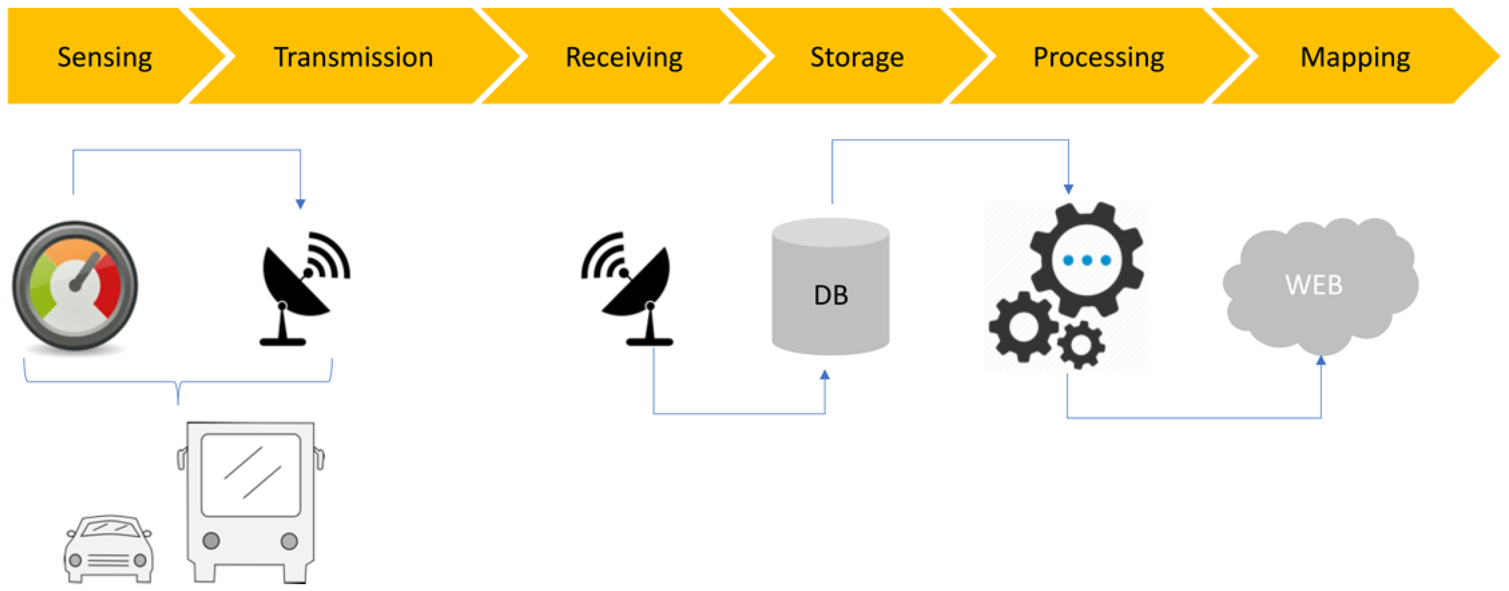
Within this work, we have developed a real-time and low-cost air quality VSN system that covers the whole path from data acquisition to data access and web-mapping. The system is named “COCAL”, after the dialectal term used for seagulls in the city of Trieste (Italy), where it has been first deployed and used [25]. COCAL consists of a set of crowdsensing low-cost internet of things (IoT) devices installed on voluntary mobile platforms (COCAL boxes). These boxes send geolocated PM measurements to an information technology (IT) infrastructure that can reconstruct, in real time, a web based interactive geographic map of the distribution of pollutants in the designated area (Figure 1).

Figure 1.
Scheme of the COCAL system and infrastructure. COCAL boxes are installed on buses and cars that contain air quality sensors and transmission devices. Data is transmitted through the mobile phone network and sent to an OGS storage and processing facility. Data products are visualized on the project’s web portal (https://cocal.ogs.it accessed on 1 November 2022).
2.1. Sensors
Traditional PM monitoring techniques, such as filters and gravimetric mass detection, are very expensive and need trained personnel and controlled procedures to correctly operate them. Providing such sensors to volunteers with no specific skills can be demotivating. In addition, installing fragile apparels in rough environments can increase costs unpredictably. LCSs are therefore needed. Unfortunately, LCSs suffer from intrinsic limitations in precision and accuracy.
Several products are available on the market and have been used and analyzed in a considerable amount of studies [22,23,42,43]. These authors demonstrated that, among LCSs, the nominal precision and accuracy of the specific brand and model of sensors can be as relevant as other external factors. The intrinsic limitations of the technology employed, the issues related to the deployment in the designated environment, and the environmental conditions can collectively introduce large errors that are very difficult to identify and prevent. It is important to note, for example, that this class of sensors is not equipped with sample conditioning devices. This has the effect that environmental conditions and relative humidity (RH), in particular, can affect hygroscopic growth of particles and bias measurements [30].
In this work, we use the SDS011 PM sensor from Nova Fitness Co.Ltd., which allows us to measure, at the same time, both PM2.5 and PM10 values. In order to monitor the environmental conditions in which the acquisition takes place, we use temperature, pressure, and RH sensors both outside and inside the COCAL box.
A detailed comparison between the performances of the SDS011 sensor and other similar sensors in controlled laboratory conditions can be found in [42]. These authors conclude that this model of sensor is suitable for air monitoring projects based on the crowdsensing approach. The same authors also carefully consider the limitations of these devices, maintaining that the precision is good while the accuracy is insufficient. In detail, this sensor tends to underestimate PM concentrations but correctly follows trends and highlights local anomalies.
To improve the accuracy of LCSs, several methods have been proposed. After an extensive survey of the existing literature on this topic, [44] maintains that only very seldomly such corrections are applied. The same author indicates that these methods are based on the use of parameters that are difficult to estimate in real life and maintains that it is also difficult to accumulate knowledge from different cases and use values obtained from one area in another area.
2.2. Data Processing and Access
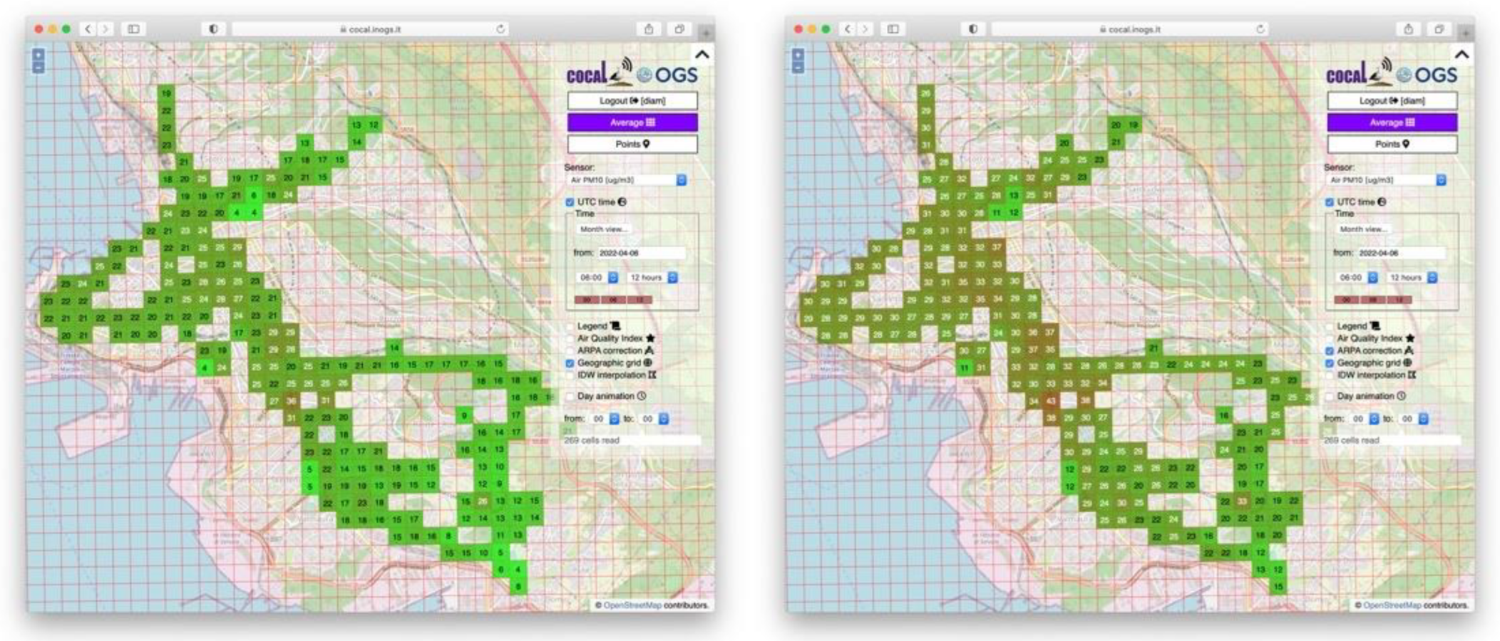
To improve the performances of our system, we devised a pragmatic two step strategy. The first step consists of automatically flagging measurements acquired in the case of problematic environmental conditions, such as when RH exceeds 70%. Thresholds are set considering the nominal technical specifications provided by the manufacturer. The second step consists in calculating the daily deviation between an official reference station and a co-located COCAL box. Since LCSs behave consistently among them, the correction can be propagated from the co-located COCAL box to the other COCAL boxes following the procedures described in [45]. The effects of the application of the corrections can be seen in Figure 2. On the left is the PM10 distribution without correction, and on the right is the PM10 distribution after the corrections.
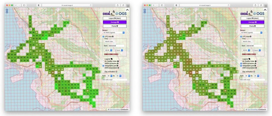
Figure 2.
Averaged PM10 distribution (left) and reference corrected distribution (right).
Once measurements have been corrected to improve LCS performances, a geographical grid of 200 × 200 m cells is superimposed on t sampling points’ distribution. Considering the measurements timeline, this is segmented into 1-h intervals, so that every set of data spanning a spatial cell and a time interval becomes a datacube. Each datacube contains measurements from different devices but refers to the same kind of sensor (e.g., PM10 or temperature). The median value of the data in each datacube is then calculated and assigned to the grid cell. This reduces the outliers, smooths values, and better represents the physical phenomena under study. A discussion on the advantages of averaging and gridding can be found in [45]. The output grid then becomes the geographic distribution of the specific parameters in the designated area in the chosen time range (Figure 2). Datacubes over longer time intervals, such as 2, 3, 4, or 8 h, are processed once a day and made available the following day.
It is important to mention that COCAL is a fully operative system that was deployed in February 2021 and has remained functional ever since. This demonstrates the feasibility, affordability, robustness, and solidity of the approach adopted. All data and data products are accessible through the interactive web portal https://cocal.ogs.it accessed on 30 October 2022. The system is fully compliant with FAIR principles and follows ISO and OGC standards.
2.3. Deployment and Coverage
Currently the COCAL network is based on five platforms installed on cars and five platforms installed on buses of the local transportation authority Trieste Trasporti. In both cases, we developed a tailored waterproof box that can be easily installed on any of the vehicles. COCAL acquisition platforms travel in the designated area with no predetermined planning. This does not mean, unfortunately, that the points of measurement follow a random geographic distribution. As a matter of fact, biases can be introduced depending on several factors such as timing, the road network, and the needs of the vehicle owners.
Regarding timing, buses have great advantages over cars. Buses cover a wide operating time, every day of the year, from five a.m. to midnight. The number of buses travelling at the same time can vary depending on the possible need for maintenance, while only seldomly does the number of active buses drop below 3 units.
Cars, to the contrary, are largely dependent on owners’ availability, which in our experience was not easy to organize. Eventually cars were not used daily, but rather, in specific time-limited periods (marathons). These marathons were planned in order to increase resolution in areas where sampling from the bus network was too coarse, or to study specific phenomena.
Regarding the spatial distribution of measurements, buses and cars behave differently. Buses follow predefined routes (bus lines) that are set up according to the socio-economic features of the urban area. If the bus network is limited geographically, or if it favors certain areas at the expense of others, then the coverage will be uneven. During the same day, each coach can be reassigned to different routes so that it can cover multiple areas of the city and the hinterland while still being limited by the bus line network.
Cars theoretically do not follow predefined routes, while this is often not the case if the data acquisition is opportunistic. In fact, when this approach is used, car owners will tend to follow their everyday schedule so that, similarly to the case of buses, a pattern will inevitably emerge. This trend can be mitigated during marathons when volunteers are asked to follow indications provided by the organizing team. Of course, this limits the freedom of participants with the risk of demotivating them [46,47,48].
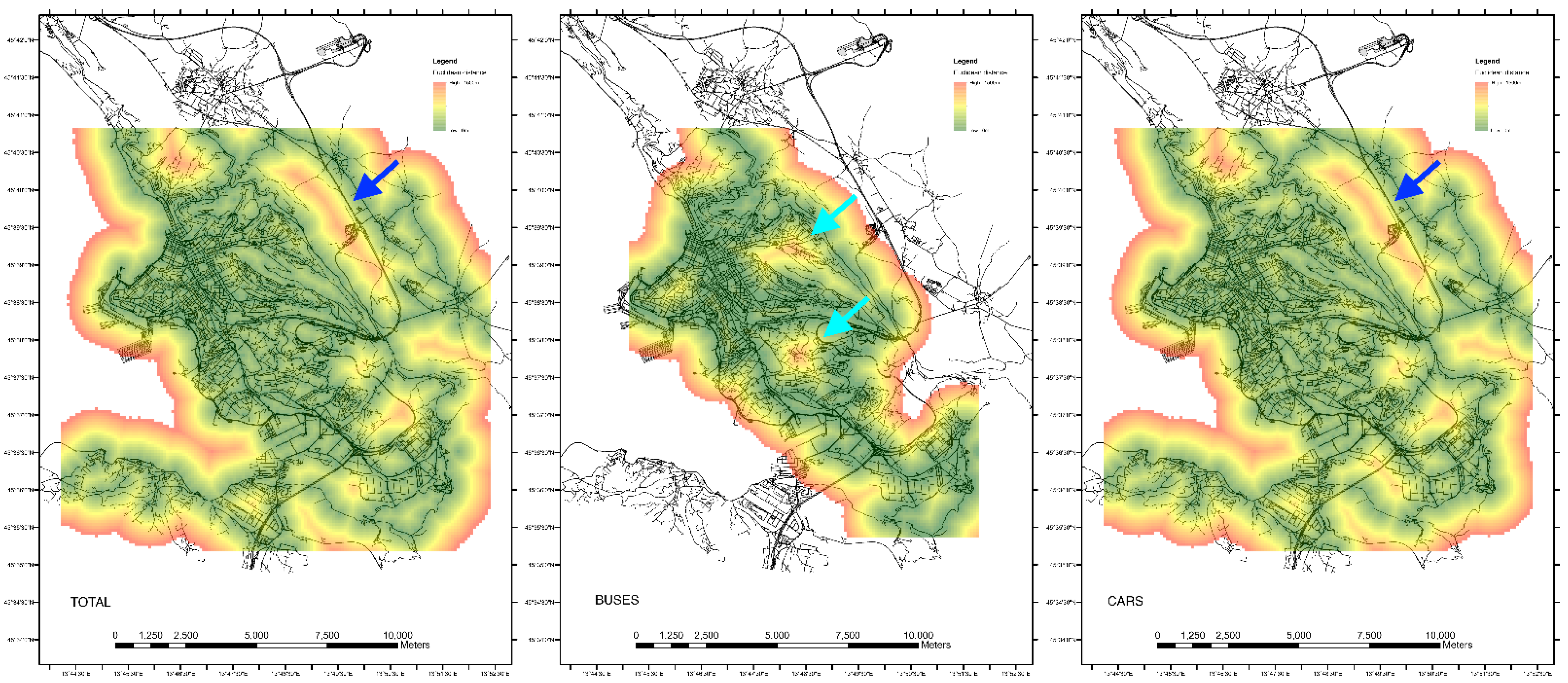
To understand how the sampling points are spatially distributed over the designated area, we will analyze measurements acquired during one single day (26 January 2022), comparing the full dataset with the separate contributions of cars and buses. After having projected the geographic position of point measurements using the EPSG:3857 spatial reference system, a first analysis of the spatial distribution of measurements can be performed by calculating the Euclidean distance (d). If, as sources we mean the location of the sampling points, the d output raster contains the measured distance from every cell to the nearest source. This map provides indications on the coverage of the designated area [49]. Where the value of d is high, sources are far from the cell position. In other words, there are gaps in the coverage. Figure 3 maps d overlaid on the road network of the City of Trieste for three cases. Figure 3 maps d for the total dataset, Figure 3 maps d only for cars, and Figure 3 maps d for buses only. Areas in green correspond to values of d that are less than 500 m and can be interpreted as areas that have a high coverage, whereas areas in yellow correspond to d ranges between 500 and 1000 m. There, coverage starts to be problematic. Cells where d is between 1000 and 1500 m are essentially gaps in the coverage and are drawn in red. In Figure 3, the map of the overall survey shows that the city center is generally well covered.

Figure 3.
Maps of Euclidean distance in the designated area calculated using the (TOTAL) full dataset, (BUSES) buses-only dataset, and (CARS) cars-only dataset. Light blue arrows mark gaps in the geographic coverage of the dataset collected by buses only. These gaps can be in-filled using the dataset collected by cars. The blue arrows mark a steep slope zone where no road can be used to collect data and therefore remain uncovered.
Focusing on the dataset collected by buses only (Figure 3), it is possible to see that the extension of the covered area is smaller than that sampled by cars. This is due to the current limited number of buses equipped with COCAL boxes. Increasing the number of installations can considerably improve the extension of the covered area. Figure 3 shows a couple of uncovered areas marked with light blue arrows. These spots are not present in Figure 3 because, differently from buses, cars were able to survey these areas. By gathering all the data available from both buses and cars, the full dataset map of d shows that gaps in buses coverage have been filled. It may be useful to analyze another type of gap such as that highlighted with a blue arrow in Figure 3. That area corresponds to a very steep slope where no road is present. No measurements can, therefore, be taken in that area using a VSN approach.
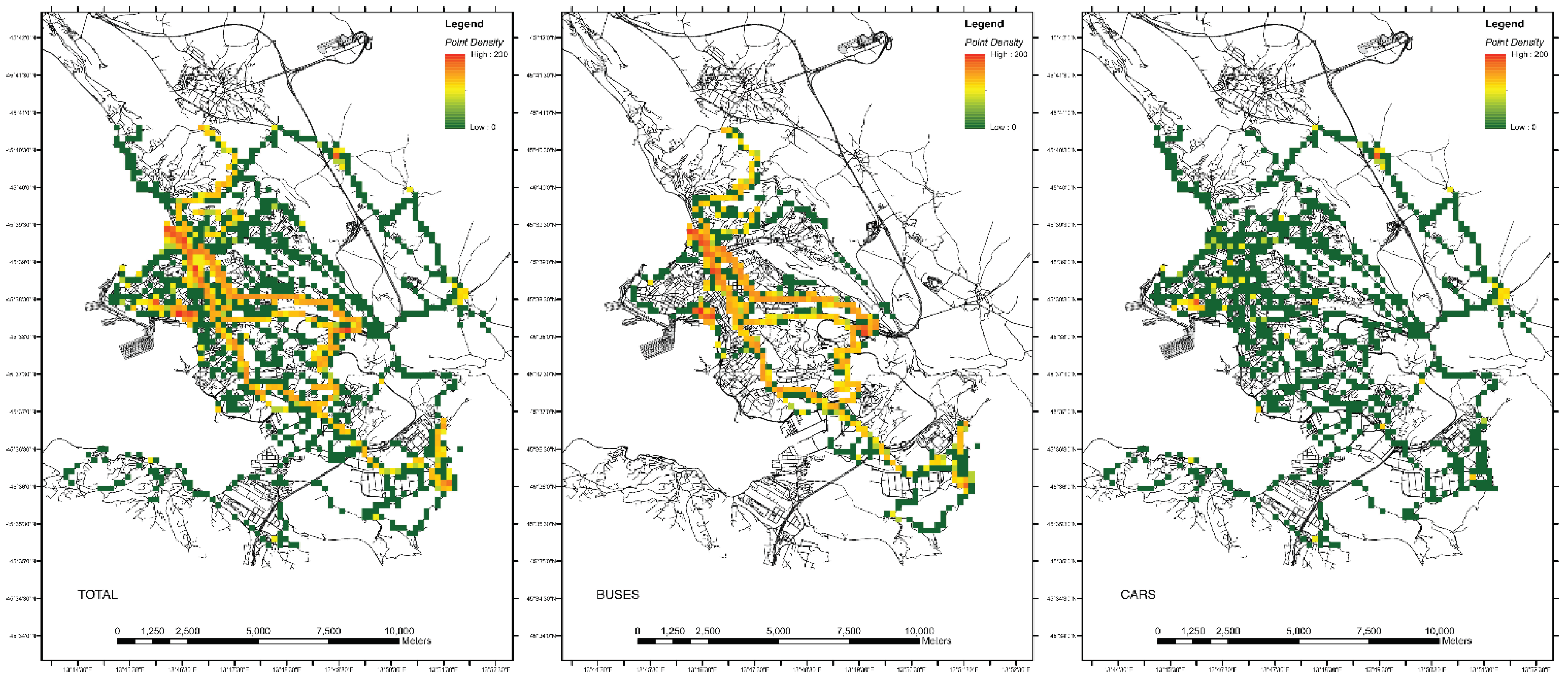
In order to understand how measurements are distributed, it is necessary to study the point density in the area. The point density is calculated by setting a neighborhood around each raster cell center, totaling the number of points that fall within the neighborhood, and dividing this value by the area of the neighborhood. The point density allows one to highlight cells where a higher number of measurements have been taken. Figure 4 shows the point density of measurements taken during the same single day of Figure 3 overlaid on the road network of the city of Trieste. Higher values of density are drawn in yellow and red.

Figure 4.
Maps of point density in the designated area calculated using the (TOTAL) full dataset, the (BUSES) buses-only dataset, and the (CARS) cars-only dataset.
There may be multiple explanations for high concentrations of points in specific areas. Data can be gathered simultaneously from multiple acquisition platforms surveying the same area (this is the case for popular traffic routes). Another possible explanation could be that platforms stop in one area for longer periods of time (this is, for example, the case for a bus line terminus, bus stops, traffic lights, or traffic jams). Figure 4 shows the density of the full dataset, Figure 4 the density of measurements taken with buses only, and Figure 4 shows measurements taken with cars only. The density of buses is very high (Figure 4—yellow and red areas), which guarantees that statistics are good. At the same time, the map shows that the geographic extension of the distribution of measurements is rather limited. This is coherent with the results of the analysis of Euclidean distances. Contrary to the case of buses, the extension of the distribution of measurements conducted with cars is wide, while the point density is much lower (Figure 4—green areas). It is easy to see that, even if the distributions of the points of measurements are different, both maps of buses and cars closely follow the road network.
It is possible to say that, while the overall coverage is good (Figure 4), large gaps exist where specific areas are not covered by roads.
So far, we have studied the Euclidean distance, which provides information on the coverage of the designated zone and the point density, which allows us to understand whether a sufficient number of measurements have been taken in an area. It is possible to make a further step and study how these measurements are distributed in terms of dispersion or clustering of measurement points. Dispersion corresponds to the case where an area is surveyed using a randomly distributed set of measurement points. Clustering corresponds to the case where sampling points are unevenly distributed. A first estimate of the type of distribution in a dataset can be derived by calculating p-values and z-scores. The p-value is the probability that the observed spatial pattern was created by some random process. A small p-value means that the observed spatial pattern is not the result of random processes. The z-score is the standard deviation of the real values from the mean value.
Very high or very low (negative) z-scores, associated with very small p-values, are found in the tails of the normal distribution. This indicates that it is unlikely that the observed spatial pattern reflects a theoretical pattern representing a complete spatial randomness point process (CSR).
We calculated p-values and z-score for the same three datasets used for the Euclidean distance and density analysis. We obtained that the full dataset shows p-value = 0.0 and z-score. = −171.7, the buses dataset shows p-value = 0.0 and z-score = −173.7, and the cars dataset shows p-value = 0.0 and z-score = −51.7. Although all three cases can be interpreted as clustered, there are differences among them. In particular, the dataset acquired with cars is less clustered than the dataset acquired with buses. This is rather simple to explain in light of the fact that buses follow predefined bus lines, while cars have more degrees of freedom. The high z-score calculated for the car traffic witnesses, at the same time, that cars cannot randomly sample an area since they are bound to a road network that will cluster the distribution of measurement points.
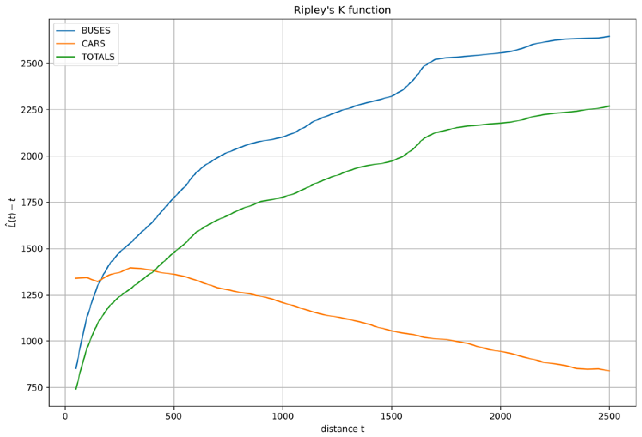
In order to understand how this bias affects the distribution of points in terms of dispersion and clustering, we studied the Ripley’s K function of the three datasets previously analyzed. The Ripley’s K function is used to compare a point pattern with a CSR point distribution over a range of distances. In Figure 5, Ripley’s K functions are plotted in light blue for buses, in orange for cars, and in green for the full dataset.
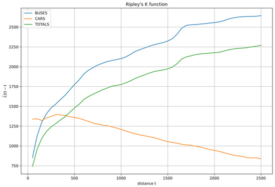
Figure 5.
Ripley’s K functions calculated for buses (light blue), cars (orange), and the full dataset (green).
The high L(t)-t values of all three cases show that all the geographic distributions of measurement points are highly clustered, while, if we also go into details in this analysis, similarly and consistently with p-values and z-scores analysis mentioned above, different behaviors can be identified for cars and buses. The dataset acquired by cars is generally less clustered than that acquired by buses. Buses show increasing values as a function of distance, while cars’ values are initially higher but soon decrease with distance. The specific behavior of cars and buses for smaller distances probably has to deal with the different frequency of stop-and-go in the city center. Bus stops, traffic lights, and other causes can push measurements into clusters.
A detailed analysis of these phenomena is beyond the scope of this paper and, in addition, it must be highlighted that these studies have some limitations. Ripley’s K analysis is, in fact, possible under the null hypothesis and the hypothesis of process stationarity [50]. It is easy to understand that both conditions are hardly satisfied in a VSN case.
The stationarity condition is particularly difficult to be met since dynamic weather conditions or the changes in position and dimension of a pollution plume can deeply challenge the assumptions made.
COCAL superimposes on the point distribution of measurements a regular square grid of 200 × 200 m cells. Cell dimensions were chosen using the maximum speed in urban areas (50 km/h) and the rate of measurement of COCAL boxes, which is 10 s. The theoretical distance between measurements was then calculated in approximately 15 m. A statistical analysis of the data acquired showed that the observed mean distance between measurements is 14.58 m, which is very close to the theoretical one. This distance guarantees that the number of measurements in each cell is approximately 10 to 12, which guarantees that averaging data within each cell is statistically feasible. Lower vehicle velocities allow one to collect more data, thus increasing redundancy, while higher vehicle velocities can be problematic. COCAL automatically detects these anomalies and flags the corresponding measurements.
The current deployment of COCAL consists of a dozen platforms. As we have shown, this imposes limitations on the covered area and the density of measurements. Increasing the number of platforms deployed can improve the situation. In this perspective, COCAL has been devised in order to be easily scaled to larger areas and to a larger number of acquisition platforms. Limitations in this sense can be related to three types of problems, namely: (i) the number of active COCAL boxes; (ii) the limitations related to the IT infrastructure; and (iii) the extension of the designated area. Increasing the number of active COCAL boxes is not only a technological issue because volunteers have to be enrolled and motivated while a congruent number of devices have to be assembled. This is not easily managed by a research institution, so possible collaborations with governmental or private organizations would definitely be helpful in this sense.
From an IT point of view, COCAL is fully integrated with real-time crowdsensing infrastructure run by Istituto Nazionale di Oceanografia e di Geofisica Sperimentale—OGS. This infrastructure manages several other types of environmental parameters, such as sea water quality [19,23] and urban and underwater anthropic noise [24]. Regular monitoring of the infrastructure has been implemented since the beginning of the project. From our experience, the stress that the COCAL initiative imposed on the infrastructure was minimal. We calculated that scaling the number of acquisition platforms by two orders of magnitude will not excessively impact the system. Scaling the initiative in order to extend the surveyed area is a more complicated topic since this implies that choices in the actual target of the study have to be made. Studying other cities to reconstruct the local pattern of traffic pollution there, for example, will be different from planning a regional survey. Different acquisition and IT strategies can be explored, in this sense, that are beyond the scope of this work.
3. Results
The technology behind COCAL was developed during 2020. During an initial phase, the trials took place using multiple simultaneous acquisition and transmission platforms mounted on vehicles operated by our institution. This allowed us to extensively test the system, its scalability, precision, and accuracy during specific targeted surveys. Once the system was finalized, we were able to deploy a fully operative system on vehicles of the local transportation authority (Trieste Trasporti) and on some voluntary cars. COCAL entered into service in February 2021 and has been fully operative ever since. Its data are fully public and can be accessed using standardized procedures from the COCAL web portal.
The main results of the work are, on one hand, the COCAL system itself and, on the other, the availability of a very large quantity of environmental measurements. COCAL was demonstrated to be efficient, robust, and easy to install and maintain, thus allowing a very high throughput of environmental data. COCAL strongly confirms that low-cost participative systems are suitable for monitoring air quality, although some precautions must be considered.
The availability of a very large quantity of environmental measurements allowed us to significantly increase the spatial and time coverage of the distribution of air pollutants in the designated area. This has made it possible to identify numerous interesting trends and local anomalies. In the following, we report on some applications that were foreseen and applied to the designated area, which have given encouraging results.
3.1. The Designated Area
The COCAL air quality system has been deployed in the urban and hinterland area of the city of Trieste (Italy), located at the northmost tip of the Adriatic Sea. The city hosts approximately 200,000 inhabitants, several industries, and one of the most active ports in the northern Adriatic Sea. From a topographic point of view, the area can be divided in two parts, namely: (i) the Karst plateau and (ii) the urban centre and outskirts. The Karst is the northwesternmost part of the External Dinarides that forms an NW–SE oriented anticlinorium [51] located at about 350 m above the sea level. The city and its industrial area, instead, lie mostly at the sea level. The area is formed mainly by limestones with a lack of surface waters. The slope between the plateau and the city in some areas can be very steep. Differences in the distribution of vegetation exist between the plateau and the urban area. This is known to have an effect on the distribution of PM and health stressors [52,53].
Relationship between Particulate Matter Distribution and Weather Condition
The designated area is generally characterised by a mild Mediterranean climate with frequent events of strong and cold northern to north-eastern katabatic wind called “Bora” [28]. The Bora can reach speeds of up to 170 km/h and can blow for several days. When these events take place, the city is swept from the hills to the sea with the effect that the polluted air masses are removed from the city area. As a consequence, the air quality in the urban area improves dramatically. On the contrary, when south-west to north-east winds are prevalent, the polluted air masses remain trapped because they find an obstacle in the hills’ slope. As a consequence, pollutants produced in the urban area and nearby industrial zones tend to accumulate. Rainfall can also improve air quality through the below-cloud aerosol scavenging process by precipitation [27,54].
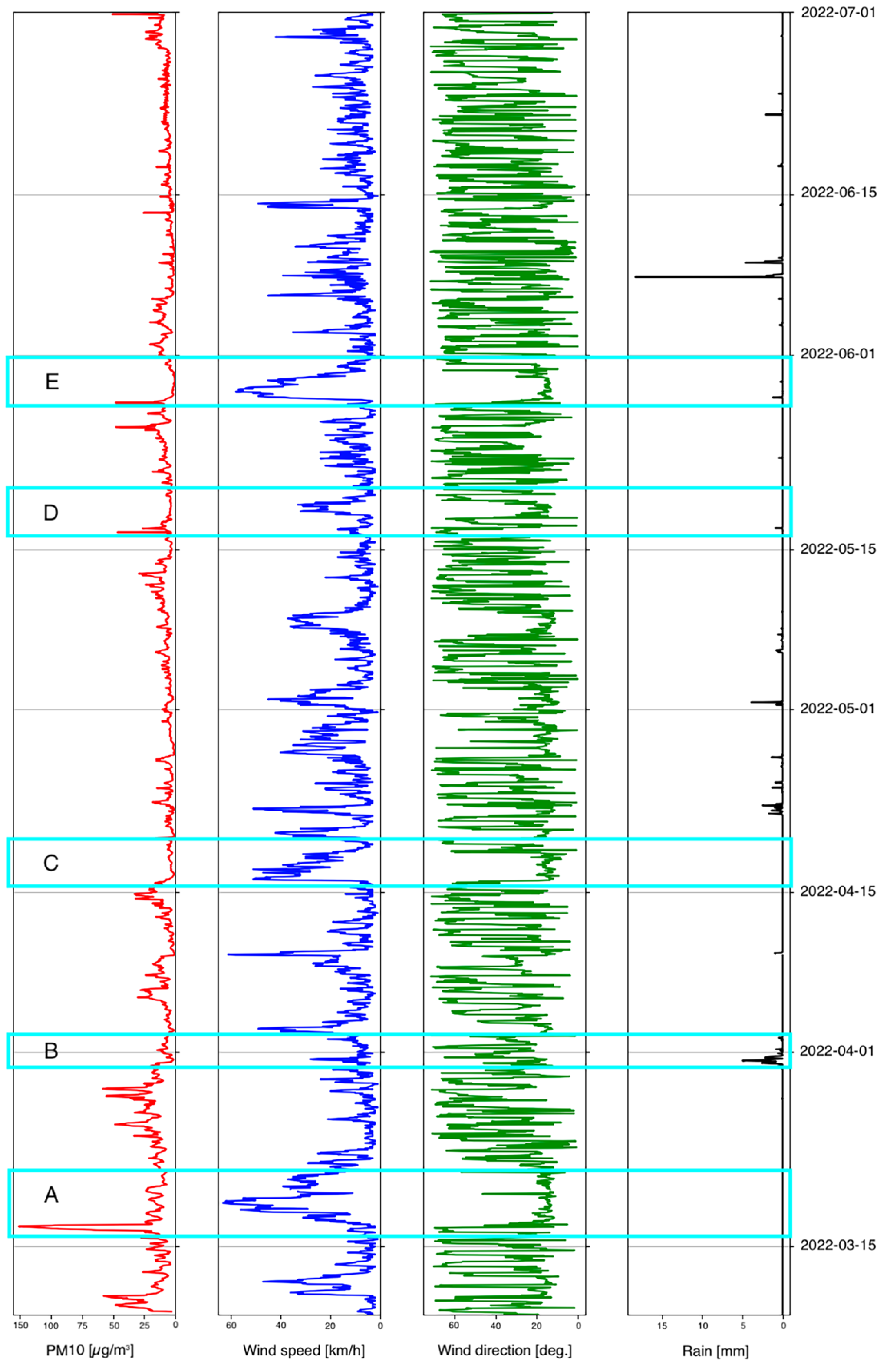
In order to highlight the importance of the weather conditions on the distribution of PM, we correlated the time series from a local meteo station (CNR-ISMAR, Molo Fratelli Bandiera (M.F.B.)) with PM time series measured at the COCAL station collocated with the governamental reference station. In Figure 6, PM10 values are drawn in red, wind speed in blue, wind direction in green, and rainfalls in black. It must be noted that, in the period of the experiment, rainfalls were very rare. This allowed us to isolate the interactions among the speed and direction of the wind with the concentration of PM. The Bora regime (NE) is identified by direction values ranging from 60 to 100 degrees and by a generally higher wind speed. It can be seen (highlighted by the light blue boxes in Figure 6) that, when the Bora speed increases, the level of PM dramatically drops. In different weather conditions, PM levels tend to increase progressively.

Figure 6.
Relationship between particulate matter distribution and weather condition. PM concentrations (red) decrease (events A, C, D, E) when the wind speed (blue) increases blowing from nort-east (Bora—green in the range between 60° and 100°). Although rainfalls (black) have been low in the considered period, effects can be seen in the event B.
3.2. Near Real-Time Local Events Monitoring
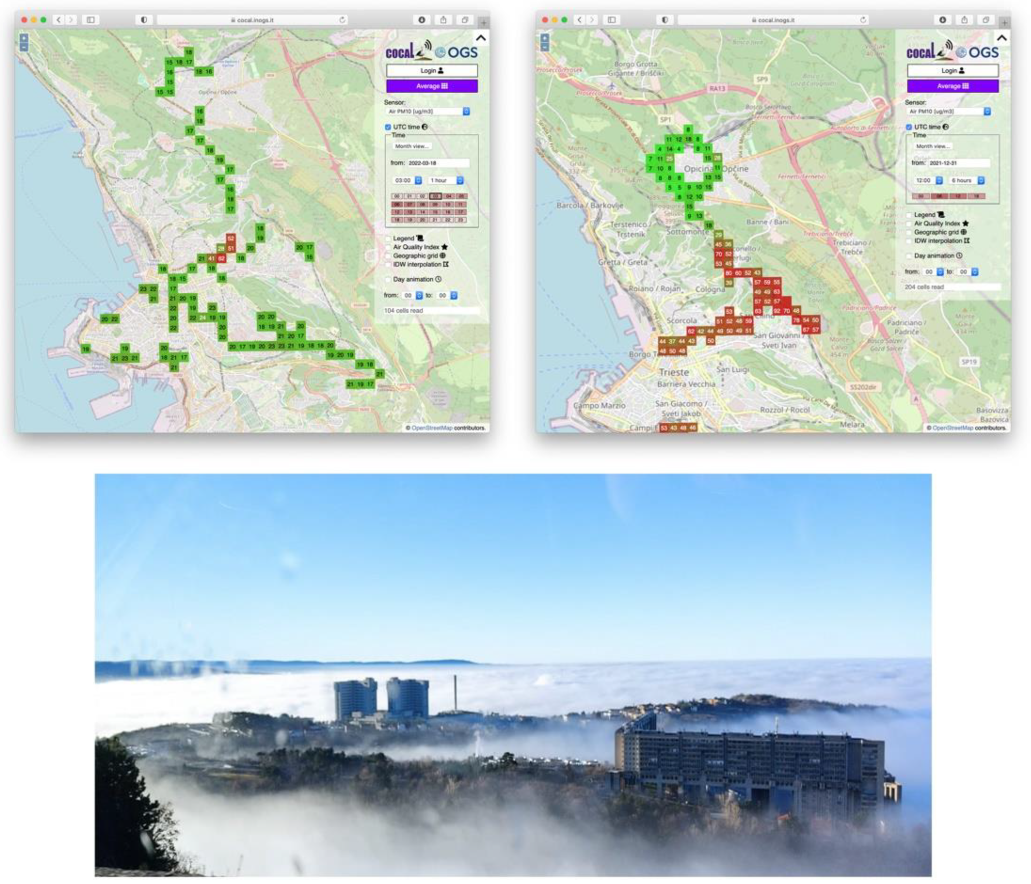
COCAL is a near-real time system that allows one to highlight anomalous events almost immediately so that dangerous situations can be handled as soon as possible. In the example of Figure 7, urgent roadworks had to be conducted on a heavily trafficked street. Closing it during the day would have resulted in long queues to access the city center. In order to avoid this situation, roadworks were moved to the evening. COCAL correctly, and with great precision, detected the anomaly. The dust resulting from roadworks can be easily identified in Figure 7 (upper left, area in red). After having spotted the situation, dust control measures in the following hours allowed the mitigation of the effects of roadworks in the surrounding areas.

Figure 7.
Examples of the application of near-real time web-based monitoring: road constructions (upper left); temperature inversion (upper right); photo of the atmospheric phenomenon from uphill (lower).
Another interesting case we detected was a temperature inversion that took place in Trieste at the end of December 2021 that triggered higher temperatures in the Karstic Plateau, relative to the urban area. This trapped the colder, humid, and polluted air masses in the urban area. The temperature inversion created a very suggestive view for those living uphill, but also a rather unhealthy situation for those living in the city centre (Figure 7). COCAL was able to detect and map this phenomenon (Figure 7) with great precision, distinguishing the clean air environment in the surroundings of the Karstic village of Opicina (Figure 7 green area) from the polluted area of the city centre (Figure 7 red area). It is very interesting to notice the sudden change in the characteristics of the distribution of air quality following the road connecting the two areas. This sudden change very closely resembles the situation shown in the photo taken from uphills (Figure 7).
3.3. Monitoring Air Quality in Relation to COVID-19 Lockdown
As the COCAL system was launched in February 2021, the system was not able to monitor the changes in air quality related to the COVID-19 lockdowns that were decided by the Italian government during 2020 and that were more generalised than those happening during 2021. Nevertheless, COCAL was able to cover the partial lockdown that occurred between 15 March 2021 and 11 April 2021 [55]. COCAL continued to be operational in that period since public transportation and environmental monitoring activities were exempted from lockdown limitations.
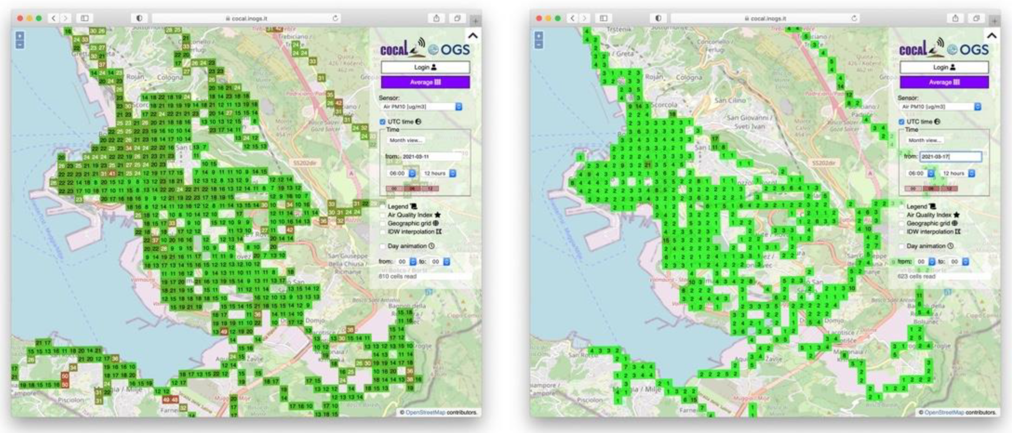
Figure 8 (left) shows the air quality distribution in the designated area on 11 March 2021 (pre-lockdown situation). This map resembles the usual distribution of air quality in the urban area during winter. Figure 8 (right) shows the situation on 17 March 2021, during the COVID lockdown, and demonstrates that PM levels were drastically reduced.

Figure 8.
Comparison between the air quality before 11 March 2021 and during 17 March 2021 (the COVID-19 lockdown was issued on 15 March 2021).
3.4. Comparison of Different Zones of the Designated Area
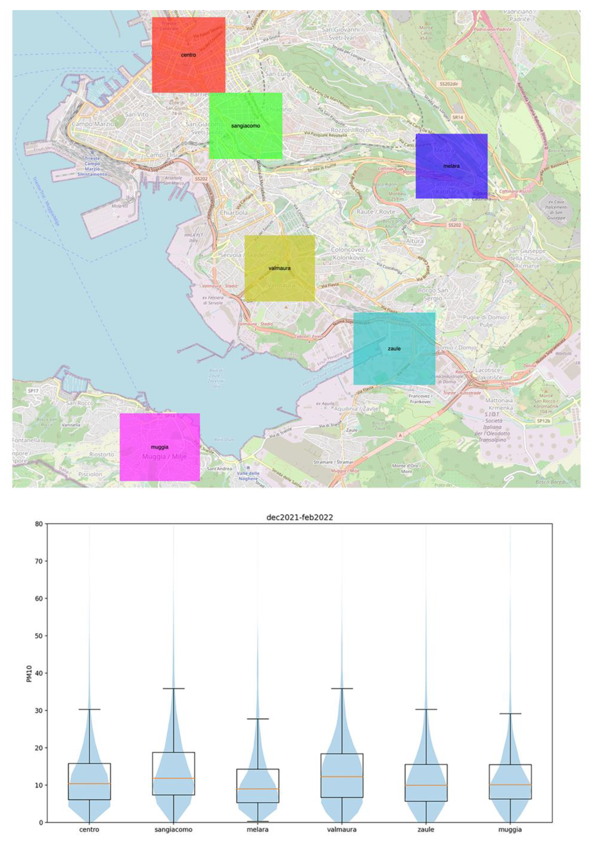
A qualitative analysis of the large amount of data we were able to collect since March 2021 highlighted that the designated area does not behave homogeneously in terms of air quality. Different parts of the city tend to accumulate air pollution in different ways. In order to understand how this actually occurs, we selected six equidimensional zones in the city and its hinterland and compared the measurements available in each of them. Figure 9 (upper) shows the positions of the considered zones. Although the density of measurements is not the same in all zones, the large amount of data collected in each zone guarantees that the results are statistically significant. The analysis focussed on the third quartile of the distribution of PM measurements in each area. Higher third quartiles can be interpreted as a tendency to perform worse in terms of air quality. This is due to the fact that frequent high levels of PM will upwardly shift the distribution of PM values. As can be easily seen in the violin plots (Figure 9, lower), the areas that show higher third quartiles are those immediately outside the urban center (San Giacomo, Valmaura), while the city center experiences lower PM concentrations.

Figure 9.
The six areas selected for the air quality comparison (upper); violin plots of PM concentrations in the different areas (lower).
4. Discussion
The large amount of data collected by COCAL highlights interesting trends and hotspots in the distribution of PM in the designated area. Unfortunately, a severe limitation of the LCSs used is the fact that they cannot perform any type of chemical analysis. Consequently, it is not possible to identify, with sufficient reliability, the sources of pollution. As a result, it is very difficult to unequivocally associate an anomaly with a cause such as urban traffic, domestic heating, or emissions from industries. However, results such as those obtained during the COVID lockdown can provide significant clues on the topic (Section 3.3).
Following [56], a daily estimate of approximately 420,000 trips in the urban area of Trieste have been calculated. Under normal conditions, 47% of them are conducted by car, 20% are conducted by public transportation, 13% are conducted by motorbike, and 20% are conducted on foot or by other means of transportation. Almost 60% of the overall trips in the urban area of Trieste can, therefore, be associated with private vehicular traffic. COVID-19 prevention rules discouraged people from driving, so it seems rather reasonable to associate the large improvement in air quality in the urban area during lockdown with the reduction of private vehicular traffic. Similar results have been obtained in other areas by several authors, such as [57,58,59], to mention just a few.
In order to further support this hypothesis and exclude a possible dependance from weather conditions, we conducted a specific review of the data available from the M.F.B. station in that period. This survey showed that the weather has always been stable, with the exception of a limited episode of 4 h on 14 March 2021. During that event, moderate winds from the north-east, with a maximum speed of 40 km/h and a maximum 5 mm of rainfall, were recorded.
During the COVID-19 lockdown, the improvement in air quality resulted in a quasi-homogeneous low level PM concentration distribution (Figure 8), whereas the distribution of PM in non-lockdown conditions shows, instead, high values that are not geographically homogeneous.
In Section 3.4, six different areas of the city that show different behavior were considered. In terms of air quality, the city center generally performs better than the urban belt immediately outside it (San Giacomo, Valmaura). A possible explanation for this behavior could be related to the fact that traffic limitations have effectively been implemented in the city center [56]. As a consequence, car traffic tends to jam in peripheral areas while awaiting to enter the city center itself. This is a reasonable explanation if we consider that the industrial area of the city is located further south (Zaule, Muggia) of the urban belt and that, in those peripheric areas, the distribution of PM measurements seems less problematic. As mentioned above, it is not possible to perform chemical analysis using LCSs. The hypothesis drawn so far cannot, therefore, be confirmed using LCS measurements alone, and further detailed chemical studied are recommended.
5. Conclusions
We developed a mobile air quality monitoring system based on a participative crowdsourcing paradigm only. The system allows to acquire, transmit, process and map, both geographically and over time, the distribution of air pollutants such as particulate matter. The system was deployed on a dozen platforms, including buses from the local transportation authority and voluntary cars. The system has been fully operational since February 2021 and has been demonstrated to be extremely robust without almost any need for maintenance.
Participatory systems must be based on low-cost sensors otherwise the expenditure of such initiatives would quickly exceed any reasonable budget. We have carefully considered all the drawbacks that this might introduce, understanding that since the accuracy of the sensors is rather low, they cannot be used to produce reference measurements. However, we verified that their precision is sufficient to identify both trends and hotspots.
In order to correct the limitations in accuracy, we developed an automatic method that takes into account the difference between the measurements taken with low-cost sensors and the official reference values taken by official environmental agencies.
The large quantity of data gathered so far constitutes an extremely important asset for understanding the dynamics of the pollution in the designated area, allowing one not only to identify sudden anomalies due to specific events, but also to identify different trends in different areas of the city. We showed that, during the COVID-19 lockdowns, a significant improvement in air quality can be correlated to the block of private car traffic, thereby also demonstrating its detrimental role on air quality.
We analyzed the large amount of data gathered since the launch of COCAL and were able to identify an urban belt where the air quality is worse than elsewhere in the city. This anomaly can also be correlated to the private car traffic, although further chemical studies are recommended to confirm this.
Our results demonstrate the impact of traffic on air quality in the designated area and that the approach we used in COCAL can be very helpful in planning mobility and transportation in collaboration with local municipalities.
Participative data collection and the availability of real-time pollution maps should make the whole city community reflect on how they can effectively help to improve the air quality in the area that they live in. It would be easier, then, to advise on, or even reinforce, the reduction of private car traffic, thereby increasing the more widespread use of public transportation.
Author Contributions
Conceptualization, P.D.; Data curation, M.I., N.P., A.V., M.B., and A.B.; Formal analysis, P.D. and M.I.; Funding acquisition, P.D.; Investigation, P.D., M.I., and R.J.C.; Methodology, P.D., M.I., and R.J.C.; Project administration, P.D.; Resources, R.J.C., N.P., A.V., and A.B.; Software, M.I. and R.J.C.; Supervision, P.D.; Validation, P.D., M.I., R.J.C., and N.P.; Visualization, M.I.; Writing—original draft, P.D., M.I., and R.J.C.; Writing—review & editing, P.D.. All authors have read and agreed to the published version of the manuscript.
Funding
This research received no external funding.
Data Availability Statement
All the data used in this work are freely and openly available from the web site https://cocal.ogs.it accessed on 30 October 2022.
Acknowledgments
The authors would like to thank Trieste Trasporti TPL, the local transportation authority of Trieste, for its support, without which this work would have not been possible. And, in particular, they would also like to thank, for their great help, Giuseppe Zottis, Fabrizio Godinich, and Fabio Vidotto. They would like, also, to very much thank the editor and anonymous reviewers for their suggestions, as well as Fausto Ferraccioli for his help in revising the text.
Conflicts of Interest
The authors declare no conflict of interest.
References
- World Health Organization. Global Status Report on Noncommunicable Diseases 2014; World Health Organization: Geneva, Switzerland, 2014; Available online: https://apps.who.int/iris/handle/10665/148114 (accessed on 11 May 2022).
- Pirozzi, C.S.; Jones, B.E.; Vanderslice, J.A.; Zhang, Y.; Paine, R., III; Dean, N.C. Short-Term Air Pollution and Incident Pneumonia. A Case–Crossover Study. Ann. Am. Thorac. Soc. 2018, 15, 449–459. [Google Scholar] [CrossRef] [PubMed]
- Neupane, B.; Jerrett, M.; Burnett, R.T.; Marrie, T.; Arain, A.; Loeb, M. Long-term exposure to ambient air pollution and risk of hospitalization with community-acquired pneumonia in older adults. Am. J. Respir. Crit. Care Med. 2010, 181, 47–53. [Google Scholar] [CrossRef] [PubMed]
- Zanobetti, A.; Schwartz, J.; Dockery, D. Airborne particles are a risk factor for hospital admissions for heart and lung disease. Environ. Health Perspect. 2000, 108, 1071–1077. [Google Scholar] [CrossRef] [PubMed]
- Brunekree, B.; Downward, G.; Forastiere, F.; Gehring, U.; Heederik, G.; Hoek, G. Air Pollution and COVID-19′. European Parliament. 2021. Available online: https://www.europarl.europa.eu/RegData/etudes/STUD/2021/658216/IPOL_STU(2021)658216_EN.pdf (accessed on 13 May 2022).
- Lim, S.; Bassey, E.; Bos, B.; Makacha, L.; Varaden, D.; Arku, R.E.; Baumgartner, J.; Brauer, M.; Ezzati, M.; Kelly, F.J.; et al. Comparing human exposure to fine particulate matter in low and high-income countries: A systematic review of studies measuring personal PM2.5 exposure. Sci. Total Environ. 2022, 833, 155207. [Google Scholar] [CrossRef] [PubMed]
- Du, Y.; Wan, Q.; Liu, H.; Liu, H.; Kapsar, K.; Peng, J. How does urbanization influence PM2.5 concentrations? Perspective of spillover effect of multi-dimensional urbanization impact. J. Clean. Prod. 2019, 220, 974–983. [Google Scholar] [CrossRef]
- Megaritis, A.; Fountoukis, C.; Charalampidis, P.; Denier Van Der Gon, H.; Pilinis, C.; Pandis, S. Linking climate and air quality over Europe: Effects of meteorology on PM2.5 concentrations. Atmos. Chem. Phys. 2014, 14, 10283–10298. [Google Scholar] [CrossRef]
- Alvarez, H.B.; Echeverría, R.S.; Alvarez, P.S.; Krupa, S. Air Quality Standards for Particulate Matter (PM) at high altitude cities. Environ. Pollut. 2013, 173, 255–256. [Google Scholar] [CrossRef]
- Miao, C.; Yu, S.; Zhang, Y.; Hu, Y.; He, X.; Chen, W. Assessing outdoor air quality vertically in an urban street canyon and its response to microclimatic factors. J. Environ. Sci. 2023, 124, 923–932. [Google Scholar] [CrossRef]
- Ito, K.; Christensen, W.F.; Eatough, D.J.; Henry, R.C.; Kim, E.; Laden, F.; Lall, R.; Larson, T.V.; Neas, L.; Hopke, P.K.; et al. PM source apportionment and health effects: 2. An investigation of intermethod variability in associations between source-apportioned fine particle mass and daily mortality in Washington, DC. J. Expo. Sci. Environ. Epidemiol. 2006, 16, 300–310. [Google Scholar] [CrossRef]
- Pope, A.; Coleman, N. Fine Particulate Air Pollution and Human Mortality_ 25+ Years of Cohort Studies|Elsevier Enhanced Reader. Available online: https://reader.elsevier.com/reader/sd/pii/S0013935119307212?token=1704793D005F9A2684CEA1B5456F9BFE5C1EC5559C6019C9EC1DDAA7CE74FAD29370C6AE975981856F1EEF7D8744FEBC&originRegion=eu-west-1&originCreation=20220513150124 (accessed on 13 May 2022).
- Singh, D.; Dahiya, M.; Kumar, R.; Nanda, C. Sensors and systems for air quality assessment monitoring and management: A review. J. Environ. Manag. 2021, 289, 112510. [Google Scholar] [CrossRef]
- Bonafè, G.; Montanari, F.; Stel, F. Air quality in Trieste, Italy—A hybrid Eulerian-Lagrangian-statistical approach to evaluate air quality in a mixed residential-industrial environment. Int. J. Environ. Pollut. 2018, 64, 246–264. [Google Scholar] [CrossRef]
- Irwin, A. Citizen Science: A Study of People, Expertise and Sustainable Development; Routledge: London, UK, 2022. [Google Scholar]
- Bonney, R.; Phillips, T.B.; Ballard, H.L.; Enck, J.W. Can citizen science enhance public understanding of science? Public Underst. Sci. 2016, 25, 2–16. [Google Scholar] [CrossRef]
- Ganti, R.K.; Ye, F.; Lei, H. Mobile crowdsensing: Current state and future challenges. IEEE Commun. Mag. 2011, 49, 32–39. [Google Scholar] [CrossRef]
- Silvertown, J. A new dawn for citizen science. Trends Ecol. Evol. 2009, 24, 467–471. [Google Scholar] [CrossRef]
- Diviacco, P.; Nadali, A.; Nolich, M.; Molinaro, A.; Iurcev, M.; Carbajales, R.; Busato, A.; Pavan, A.; Grio, L.; Malfatti, F. Citizen science and crowdsourcing in the field of marine scientific research—The MaDCrow project. J. Sci. Commun. 2021, 20, A09. [Google Scholar] [CrossRef]
- Stewart, C.; Labrèche, G.; González, D. A Pilot Study on Remote Sensing and Citizen Science for Archaeological Prospection. Remote Sens. 2020, 12, 2795. [Google Scholar] [CrossRef]
- Froeling, F.; Gignac, F.; Hoek, G.; Vermeulen, R.; Nieuwenhuijsen, M.; Ficorilli, A.; De Marchi, B.; Biggeri, A.; Kocman, D.; Robinson, J.A.; et al. Narrative review of citizen science in environmental epidemiology: Setting the stage for co-created research projects in environmental epidemiology. Environ. Int. 2021, 152, 106470. [Google Scholar] [CrossRef]
- Fraisl, D.; Hager, G.; Bedessem, B.; Gold, M.; Hsing, P.-Y.; Danielsen, F.; Hitchcock, C.B.; Hulbert, J.M.; Piera, J.; Spiers, H.; et al. Citizen science in environmental and ecological sciences. Nat. Rev. Methods Primer 2022, 2, 264. [Google Scholar] [CrossRef]
- Diviacco, P.; Nadali, A.; Iurcev, M.; Carbajales, R.; Busato, A.; Pavan, A.; Burca, M.; Grio, L.; Nolich, M.; Molinaro, A.; et al. MaDCrow, a Citizen Science Infrastructure to Monitor Water Quality in the Gulf of Trieste (North Adriatic Sea). Front. Mar. Sci. 2021, 8, 619898. [Google Scholar] [CrossRef]
- Diviacco, P.; Nadali, A.; Iurcev, M.; Burca, M.; Carbajales, R.; Gangale, M.; Busato, A.; Brunetti, F.; Grio, L.; Viola, A.; et al. Underwater Noise Monitoring with Real-Time and Low-Cost Systems, (The CORMA Experience). J. Mar. Sci. Eng. 2021, 9, 390. [Google Scholar] [CrossRef]
- Diviacco, P.; Iurcev, M.; Carbajales, R.J.; Potleca, N. First results of the application of a citizen science based mobile monitoring system to the study of household heating emissions. Atmosphere 2022, 13, 1689. [Google Scholar] [CrossRef]
- PKanaroglou, P.S.; Jerrett, M.; Morrison, J.; Beckerman, B.; Arain, M.A.; Gilbert, N.L.; Brook, J.R. Establishing an air pollution monitoring network for intra-urban population exposure assessment: A location-allocation approach. Atmos. Environ. 2005, 39, 2399–2409. [Google Scholar] [CrossRef]
- Gao, B.; Ouyang, W.; Cheng, H.; Xu, Y.; Lin, C.; Chen, J. Interactions between rainfall and fine particulate matter investigated by simultaneous chemical composition measurements in downtown Beijing. Atmos. Environ. 2019, 218, 117000. [Google Scholar] [CrossRef]
- Carminati, M.; Pedalà, L.; Bianchi, E.; Nason, F.; Dubini, G.; Cortelezzi, L.; Ferrari, G.; Sampietro, M. Capacitive detection of micrometric airborne particulate matter for solid-state personal air quality monitors. Sens. Actuators Phys. 2014, 219, 80–87. [Google Scholar] [CrossRef]
- Liu, X.; Jayaratne, R.; Thai, P.; Kuhn, T.; Zing, I.; Christensen, B.; Lamont, R.; Dunbabin, M.; Zhu, S.; Gao, J.; et al. Low-cost sensors as an alternative for long-term air quality monitoring. Environ. Res. 2020, 185, 109438. [Google Scholar] [CrossRef] [PubMed]
- Mead, M.; Popoola, O.; Stewart, G.; Landshoff, P.; Calleja, M.; Hayes, M.; Baldovi, J.; McLeod, M.; Hodgson, T.; Dicks, J.; et al. The use of electrochemical sensors for monitoring urban air quality in low-cost, high-density networks. Atmos. Environ. 2012, 70, 186–203. [Google Scholar] [CrossRef]
- Miskell, G.; Salmond, J.; Williams, D.E. Low-cost sensors and crowd-sourced data: Observations of siting impacts on a network of air-quality instruments. Sci. Total Environ. 2017, 575, 1119–1129. [Google Scholar] [CrossRef]
- Schneider, P.; Castell, N.; Vogt, M.; Dauge, F.R.; Lahoz, W.A.; Bartonova, A. Mapping urban air quality in near real-time using observations from low-cost sensors and model information. Environ. Int. 2017, 106, 234–247. [Google Scholar] [CrossRef]
- Sensor.Community. Build Your Own Sensor and Join the Worldwide Civic Tech Network. Available online: https://sensor.community/en/ (accessed on 13 October 2022).
- Sistemas de Monitoreo Ambiental Inteligente|AirFlux. AirFlux—Sistemas de Monitoreo Ambiental Inteligente. Available online: https://www.airflux.cl/ (accessed on 13 October 2022).
- Yi, W.Y.; Lo, K.M.; Mak, T.; Leung, K.S.; Leung, Y.; Meng, M.L. A Survey of Wireless Sensor Network Based Air Pollution Monitoring Systems. Sensors 2015, 15, 31392–31427. [Google Scholar] [CrossRef]
- González, E.; Casanova-Chafer, J.; Romero, A.; Vilanova, X.; Mitrovics, J.; Llobet, E. LoRa Sensor Network Development for Air Quality Monitoring or Detecting Gas Leakage Events. Sensors 2020, 20, 6225. [Google Scholar] [CrossRef]
- Murty, R.N.; Mainland, G.; Rose, I.; Chowdhury, A.R.; Gosain, A.; Bers, J.; Welsh, M. CitySense: An Urban-Scale Wireless Sensor Network and Testbed. In Proceedings of the 2008 IEEE Conference on Technologies for Homeland Security, Waltham, MA, USA, 12–13 May 2008; pp. 583–588. [Google Scholar] [CrossRef]
- Jiang, Y.; Shang, L.; Li, K.; Tian, L.; Piedrahita, R.; Yun, X.; Mansata, O.; Lv, Q.; Dick, R.P.; Hannigan, M. MAQS: A personalized mobile sensing system for indoor air quality monitoring. In Proceedings of the 13th International Conference on Ubiquitous Computing, New York, NY, USA, 17–21 September 2011; pp. 271–280. [Google Scholar] [CrossRef]
- Liu, R.; Pan, J. AirQ: A Privacy-Preserving Truth Discovery Framework for Vehicular Air Quality Monitoring. In Proceedings of the 2020 16th International Conference on Mobility, Sensing and Networking (MSN), Tokyo, Japan, 17–19 December 2020; pp. 65–72. [Google Scholar] [CrossRef]
- Cruz, P.; Couto, R.S.; Costa, L.H.M.K.; Fladenmuller, A.; De Amorim, M.D. Per-Vehicle Coverage in a Bus-Based General-Purpose Sensor Network. IEEE Wirel. Commun. Lett. 2020, 9, 1019–1022. [Google Scholar] [CrossRef]
- Balen, J.; Ljepic, S.; Lenac, K.; Mandzuka, S. Air Quality Monitoring Device for Vehicular Ad Hoc Networks: EnvioDev. Int. J. Adv. Comput. Sci. Appl. 2020, 11, 580–590. [Google Scholar] [CrossRef]
- Bulot, F.M.J.; Russell, H.S.; Rezaei, M.; Johnson, M.S.; Ossont, S.J.J.; Morris, A.K.R.; Basford, P.J.; Easton, N.H.C.; Foster, G.L.; Loxham, M.; et al. Laboratory Comparison of Low-Cost Particulate Matter Sensors to Measure Transient Events of Pollution. Sensors 2020, 20, 2219. [Google Scholar] [CrossRef] [PubMed]
- Zimmerman, N. Tutorial: Guidelines for implementing low-cost sensor networks for aerosol monitoring. J. Aerosol Sci. 2022, 159, 105872. [Google Scholar] [CrossRef]
- Liang, L. Calibrating low-cost sensors for ambient air monitoring: Techniques, trends, and challenges. Environ. Res. 2021, 197, 111163. [Google Scholar] [CrossRef] [PubMed]
- Iurcev, M.; Pettenati, F.; Diviacco, P. Improved automated methods for near real-time mapping—Application in the environmental domain. Bull. Geophys. Oceanogr. 2021, 62, 427–454. [Google Scholar] [CrossRef]
- Lee, L.; Darch, P. One of a kind: The tail of citizen science volunteers. Proc. Assoc. Inf. Sci. Technol. 2019, 56, 445–449. [Google Scholar] [CrossRef]
- Latifi, G.R.; Monfared, M.P.; Khojasteh, H.A. Gamification and citizen motivation and vitality in smart cities: A qualitative meta-analysis study. GeoJournal 2022, 87, 1217–1230. [Google Scholar] [CrossRef]
- KMintz, K.K.; Arazy, O.; Malkinson, D. Multiple forms of engagement and motivation in ecological citizen science. Environ. Educ. Res. 2022, 1–18. [Google Scholar] [CrossRef]
- Pang, T.T.P.; Lee, S.S. Measuring the geographic coverage of methadone maintenance programme in Hong Kong by using geographic information system (GIS). Int. J. Health Geogr. 2008, 7, 5. [Google Scholar] [CrossRef][Green Version]
- Ripley, B.D. The Second-Order Analysis of Stationary Point Processes. J. Appl. Probab. 1976, 13, 255–266. [Google Scholar] [CrossRef]
- Jurkovšek, B.; Biolchi, S.; Furlani, S.; Kolar-Jurkovšek, T.; Zini, L.; Jež, J.; Tunis, G.; Bavec, M.; Cucchi, F. Geology of the Classical Karst Region (SW Slovenia–NE Italy). J. Maps 2016, 12 (Suppl. 1), 352–362. [Google Scholar] [CrossRef]
- Terre-Torras, I.; Recalde, M.; Díaz, Y.; de Bont, J.; Bennett, M.; Aragón, M.; Cirach, M.; O’Callaghan-Gordo, C.; Nieuwenhuijsen, M.J.; Duarte-Salles, T. Air pollution and green spaces in relation to breast cancer risk among pre and postmenopausal women: A mega cohort from Catalonia. Environ. Res. 2022, 214, 113838. [Google Scholar] [CrossRef] [PubMed]
- Markevych, I.; Schoierer, J.; Hartig, T.; Chudnovsky, A.; Hystad, P.; Dzhambov, A.M.; de Vries, S.; Triguero-Mas, M.; Brauer, M.; Nieuwenhuijsen, M.J.; et al. Exploring pathways linking greenspace to health: Theoretical and methodological guidance. Environ. Res. 2017, 158, 301–317. [Google Scholar] [CrossRef]
- Luan, T.; Guo, X.; Zhang, T.; Guo, L. Below-Cloud Aerosol Scavenging by Different-Intensity Rains in Beijing City. J. Meteorol. Res. 2019, 33, 126–137. [Google Scholar] [CrossRef]
- ‘Gazzetta Ufficiale’. Available online: https://www.gazzettaufficiale.it/eli/id/2021/03/02/21A01331/sg (accessed on 3 August 2022).
- Bernetti, G.; Randazzo, L.; Borgogna, S. Piano Generale del Traffico Urbano. Regione Autonoma Friuli Venezia Giulia, Comune di Trieste. Available online: https://www.comune.trieste.it/media/files/032006/attachment/All_01_RT_rev1.pdf (accessed on 18 October 2022).
- Rys, A.; Samek, L.; Stegowski, Z.; Styszko, K. Comparison of concentrations of chemical species and emission sources PM2.5 before pandemic and during pandemic in Krakow, Poland. Sci. Rep. 2022, 12, 16481. [Google Scholar] [CrossRef] [PubMed]
- Schatke, M.; Meier, F.; Schröder, B.; Weber, S. Impact of the 2020 COVID-19 lockdown on NO2 and PM10 concentrations in Berlin, Germany. Atmos. Environ. 2022, 290, 119372. [Google Scholar] [CrossRef] [PubMed]
- Li, K.; Ni, R.; Jiang, T.; Tian, Y.; Zhang, X.; Li, C.; Xie, C. The regional impact of the COVID-19 lockdown on the air quality in Ji’nan, China. Sci. Rep. 2022, 12, 12099. [Google Scholar] [CrossRef]
Publisher’s Note: MDPI stays neutral with regard to jurisdictional claims in published maps and institutional affiliations. |
© 2022 by the authors. Licensee MDPI, Basel, Switzerland. This article is an open access article distributed under the terms and conditions of the Creative Commons Attribution (CC BY) license (https://creativecommons.org/licenses/by/4.0/).

