Abstract
Wave-dissipating blocks are the armor elements of breakwaters that protect beaches, ports, and harbors from erosion by waves. Monitoring the poses of individual wave-dissipating blocks benefits the accuracy of the block supplemental work plan, recording of the construction status, and monitoring of long-term pose change in blocks. This study proposes a deep-learning-based approach to detect individual blocks from large-scale three-dimensional point clouds measured with a pile of wave-dissipating blocks placed overseas and underseas using UAV photogrammetry and a multibeam echo-sounder. The approach comprises three main steps. First, the instance segmentation using our originally designed deep convolutional neural network partitions an original point cloud into small subsets of points, each corresponding to an individual block. Then, the block-wise 6D pose is estimated using a three-dimensional feature descriptor, point cloud registration, and CAD models of blocks. Finally, the type of each segmented block is identified using model registration results. The results of the instance segmentation on real-world and synthetic point cloud data achieved 70–90% precision and 50–76% recall with an intersection of union threshold of 0.5. The pose estimation results on synthetic data achieved 83–95% precision and 77–95% recall under strict pose criteria. The average block-wise displacement error was 30 mm, and the rotation error was less than . The pose estimation results on real-world data showed that the fitting error between the reconstructed scene and the scene point cloud ranged between 30 and 50 mm, which is below 2% of the detected block size. The accuracy in the block-type classification on real-world point clouds reached about 95%. These block detection performances demonstrate the effectiveness of our approach.
1. Introduction
Breakwaters protect beaches, ports, and harbors from erosion caused by waves. Wave-dissipating blocks made of large concrete slabs are essential components of the armor layer of breakwaters that protect their core from direct wave attacks. However, long-term wave motion and erosion damage the blocks irreversibly, causing them to sink and even break off [1]. Therefore, periodical supplemental work must be conducted on wave-dissipating blocks to maintain breakwaters. Therein, new wave-dissipating blocks are stacked onto the existing ones until their top surfaces exceed the target height, as shown in Figure 1a. Thus, precisely estimating the current block-stacking status is imperative for monitoring long-term block movements in the maintenance and planning of lean supplemental work.

Figure 1.
Supplemental work on wave-dissipating blocks. Periodical repair work aims at stacking new supplemental blocks on top of existing ones until the target height. (a) Block supplemental work; (b) Three-dimensional (3D) measurement of existing block surface; (c) Individual block pose detection.
With the recent increased availability of various 3D sensors, such as airborne LiDAR and UAV photogrammetry, dense three-dimensional (3D) point clouds of existing offshore object surfaces can be easily measured at a low cost [2]. Conversely, the multibeam echo-sounder (MBES) enables capturing a large-scale 3D point cloud of the bottom of water and realizes a detailed exploration of undersea objects [3,4]. Moreover, drone-mounted RGB and multispectral imagery [5] and drone-mounted lightweight dual-wavelength LiDAR systems [6] enable shallow bathymetric mapping capabilities and undersea object detection. The data integration effectiveness of bathymetric mapping using a single-beam echo-sounder with ground surface mapping using terrestrial LiDAR and UAV photogrammetry has also been demonstrated [7].
From the viewpoint of practicality and ease of use among the above 3D sensing methods, as shown in Figure 1b, the emergent areas of wave-dissipating blocks can be measured easily by UAV photogrammetry, while MBES can measure the submerged portion. Suppose that individual block poses can be detected from the measured point clouds of existing block surfaces, as shown in Figure 1c. This allows the evaluation of more precise overseas and undersea block-wise stacking status required for long-term maintenance and a lean supplemental plan.
Accurate monitoring of the poses of individual wave-dissipating blocks offers the following benefits for the administrators:
- The 6D poses of individual blocks faithfully reproduce the as-built status of each block to improve the accuracy of estimates of new blocks’ quantities and their stacking plan in the supplemental work;
- The as-built status can be grasped block by block after the construction and supplemental works. Thus, the construction results can be recorded and visualized comprehensively compared to recording only the measured point clouds of existing block surfaces;
- By providing the pose and attribute information to each block model, it is possible to check the long-term change in the blocks, such as missing, sinking, and damaged blocks, and implement a more precise and sustainable maintenance activity.
To date, several studies compared the dense 3D point clouds acquired at different times [2,8,9,10,11,12] to evaluate possible changes in stacked block surfaces within a certain period. However, these studies do not provide sufficient information for individual block movements or block breakage over a long time interval or after severe events [11] that could significantly affect the structural integrity of breakwaters. Due to the technical difficulty, very few studies attempted to detect individual wave-dissipating block poses from 3D dense point clouds. For example, Bueno et al. [1] presented an algorithm for reconstructing cube-shaped wave-dissipating blocks from incomplete point clouds captured by airborne LiDAR. Shen et al. [13] estimated individual brick poses from laser-scanned point clouds that measured a cluttered pile of cuboid bricks. Although the above methods can recognize blocks with simple shapes, it is difficult for them to identify those with complex shapes, such as tetrapods or clinger blocks.
To address this issue, a novel deep-learning-based 3D pose detection method of wave-dissipating blocks from as-built point clouds measured by UAV-photogrammetry and MBES with reasonable detection performances is designed and proposed. The method can detect as many blocks as possible all at once from a given scene. The proposed pose detection method enables 6D pose estimation of blocks and block-type classification.
To realize our detection method, a category-agnostic instance segmentation network called Fast Point Cloud Clustering v2 (FPCCv2) was designed initially to segment a point cloud corresponding to a block instance from point clouds measured from large areas by UAV and MBES. FPCCv2 is an instance segmentation network for point clouds extended from our previous segmentation network Fast Point Cloud Clustering (FPCC) [14] with a novel feature extractor. This feature extractor increases each point’s receptive field to obtain more discriminative features for the instance segmentation. FPCCv2 is trained on synthetic block-stacking scenes constructed from block CAD models and applied to the instance segmentation of the blocks of real scenes. The 6D pose of the segmented block is estimated using a 3D feature descriptor Point Pair Feature (PPF) [15] and refined by best-fit point cloud alignment, which is called Iterative Closest Points (ICP) [16]. Finally, a fitness score is used to distinguish each block type in a scene including different types of blocks.
The proposed block detection method is validated on three sites of ports, consisting of different block types. The instance-labeled training dataset used to supervise the network is automatically generated by a physics engine [17] and block CAD models, which avoids laborious manual labeling work on the real scene and secures rich training datasets for our network. Different synthetic point clouds are generated according to the measurement properties of UAV or MBES to bridge the gap between synthetic and real scenes. The combination of PPF and ICP enables the precise estimation of 6D poses of individual blocks in a scene. Moreover, the each block type can be identified from a point cloud scene.
In summary, the original contributions of the proposed method are described as follows:
- The originally proposed convolutional neural network called FPCCv2 enables the rapid segmentation of individual wave-dissipating block instances from a large-scale 3D measured point cloud captured from a scene of stacked blocks. This enables us to estimate 6D poses of multiple blocks at once and improve computational efficiency of the block pose estimation.
- A physics engine enables the synthetic and automatic generation of instance-labeled training datasets for the instance segmentation of blocks. It thus avoids laborious manual labeling work and secures rich training datasets for our convolutional neural network.
- Synthetic point cloud generation considering the difference in characteristics of measurement using UAV and MBES enhances the performance of instance segmentation.
- The combination of the 3D feature descriptor by PPF and point-to-point registration by ICP enables the precise estimation of 6D poses of individual blocks in a scene. Moreover, the difference in the type and size of individual blocks can be identified in a scene. This is useful for the as-built inspection and instance-level monitoring of wave-dissipating blocks.
- The performances of 6D pose estimation of individual wave-dissipating blocks are evaluated both in synthetic scenes and various real construction sites including undersea blocks.
The remainder of this paper is organized as follows. Section 2 reviews related work and clarifies the issues encountered. Section 3 introduces an overview of the proposed pose detection method. Section 4 describes our convolutional neural network used for the instance segmentation of measured point clouds. Section 5 presents the details of block pose estimation and block-type classification. Section 6 provides experimental results about detection performances using real and synthesized scenes. Finally, Section 7 presents the conclusion and future directions for research.
2. Related Work
From a geometric processing viewpoint, this study employs three techniques: (1) 3D monitoring of wave-dissipating blocks in breakwaters, mainly used in civil engineering, (2) instance segmentation on point clouds, and (3) 3D object detection and 6D pose estimation on point clouds, mainly used in computer vision. In this section, the related work on these techniques is introduced, and challenges faced by these techniques when applied to detect the 3D poses of wave-dissipating blocks from large-scale point clouds are elucidated.
2.1. Three-Dimensional (3D) Monitoring of Wave-Dissipating Blocks in Breakwaters
As stated in the introduction, wave-dissipating blocks of breakwaters require periodic monitoring and supplemental work to ensure that they remain in good condition [2,8,18,19,20]. To this end, in recent years, several studies have been reported on the use of photogrammetry and UAVs to monitor the 3D condition of blocks of breakwaters.
Sousa et al. [8] developed a data acquisition system to capture 3D point clouds of breakwaters using UAV-based photogrammetry. Lemos et al. [21] used a terrestrial laser scanner, photogrammetry, and a consumer-grade RGBD sensor to determine the rocking and displaced wave-dissipating blocks in the breakwater structure. These studies monitor block surfaces’ overall condition by comparing changes in data from different periods. However, they could not assess the state nor estimate the pose of an individual block.
In contrast, methods have gradually been proposed to investigate the condition of individual blocks in breakwaters and estimate their posture from 3D point clouds obtained by laser scanners or photogrammetry. González-Jorge et al. [2] evaluated the measurement accuracy of 3D point clouds obtained by photogrammetry and clarified the detection limit of small translations and rotations on a flat surface of one cube armor, which were manually segmented from a point cloud. Shen et al. [13] proposed an algorithm to extract individual rectangular bricks from a dense point cloud sampled from an unorganized pile of bricks using a terrestrial laser scanner. Bueno et al. [22] developed a method for the automatic modeling of breakwaters with cube-shaped block armors from a 3D point cloud captured by a terrestrial laser scanner. Unfortunately, the detection methods proposed in [2,13,22] are only applicable to a simple block, whose shape is bounded by planes. This cannot be easily extended to the recognition of blocks such as tetrapods or accropodes, whose shape is composed of complex surfaces. Moreover, low recall and high computational overhead reduce the practicality of these methods.
Recently, Musumeci et al. [12] used a consumer-grade RBGD sensor to measure the damage in a laboratory-scale model of stacked accropode blocks around a rubble mound breakwater simultaneously above and below the water level. Although they quantified the distribution of rotational and translational shifts between the point clouds captured at different times, they evaluated them only as a directional and positional shift at the centroid of a local point cloud in a small cube, which is regularly partitioned from the original point cloud. Therefore, their method could not detect individual wave-dissipating block poses from 3D dense point clouds nor quantify the individual block movements or breakage over time.
In summary, the shortcomings of research on conventional block monitoring methods are the followings: (1) They cannot detect individual blocks or their poses from point clouds. (2) Even when they can detect, the detection accuracy is low and requires several hours of computation. (3) The detectable block shapes are limited to simple shapes such as cubes, and there is no versatility in the detection method. These shortcomings make it difficult to deploy in a real-world environment.
Compared to those, the advantages of the proposed method can be summarized as follows: (1) It can identify individual block regions, poses, and their block type. (2) Its higher block detection rate and shorter computation time than conventional methods can deploy in real environments. (3) It can flexibly detect blocks with complex shapes simply by changing the block CAD model used. These advantages contribute practical, precise, and long-term monitoring of wave-dissipating blocks in the real world.
2.2. Instance Segmentation on Point Cloud
Detecting point subsets that correspond to an individual wave-dissipating block from an original point cloud can be regarded as a 3D instance segmentation problem. The 3D instance segmentation algorithm aims at assigning a label to each point in an original point cloud, distinguishing different instances of the same class.
Most deep learning-based 3D instance segmentation frameworks recently focused on indoor data and exhibited remarkable performances. For example, some grouping-based methods [23,24,25,26,27] cluster points in a high-dimensional space based on their similarity of features, while others [28,29] cluster points in Euclidean space after moving points toward their corresponding instance centers based on the predicted offset vector. These methods [23,24,25,26,27,28,29] used publicly available labeled point cloud datasets [30,31,32] as training sets developed for indoor scene segmentation. The object surfaces in these high-quality indoor point cloud scenes [30,31,32] are densely sampled with little occlusions and sometimes attached with additional information, such as RGB attributes.
However, the lower sides of actual wave-dissipating blocks stacked on coast sides cannot be measured, and missing portions of the point cloud remain, as only the upper sides of each block are measured. Therefore, the coverage of the measured points of the wave-dissipating blocks is incomplete and considerably different from the one of indoor objects. Thus, the learning-based 3D instance segmentations developed for indoor scenes [23,24,25,26,27,28,29] do not necessarily work well for the block instance segmentation of point clouds of stacked wave-dissipating blocks in the natural environment.
Recently, Ref. [33] proposed a method based on a deep neural network for the instance segmentation of LiDAR point clouds of street-scale outdoor scenes into point cloud instances of pedestrians, roads, cars, bicycles, etc. The authors used not only the labeled point cloud of real scenes but simulated scenes as well. In [33], they combined the point clouds measured from real backgrounds with the foreground 3D object models to generate their training data. However, their foreground objects are positioned separately, not jumbled, and not overlapped like wave-dissipating blocks. Moreover, they manually cleaned up the background points to remove moving objects, such as cars. Therefore, it is difficult to directly apply their method of training dataset creation and instance segmentation to our instance segmentation problem of complex overlapping blocks.
There are instance segmentation methods specifically designed according to the complexity of outdoor scenes and according to characteristics of the objects of interest. Walicka et al. [34] designed a method for segmenting individual stone grains on a riverbed from a terrestrial laser-scanned point cloud. After the random forest algorithm separates the grain and the background, a density-based spatial clustering algorithm then segments the individual grains. Luo et al. [35] first employed a neural network to segment tree points from the raw urban point cloud and then classified the tree clusters into single and multiple tree clusters according to the number of detected tree centers. Djuricic et al. [36] developed an automated analysis method to detect and count individual oyster shells placed on a fossil oyster reef from a terrestrial laser-scanned point cloud based on the convex surface segmentation from the point cloud and the openness feature. However, these segmentation algorithms are designed to segment the instances of specific objects in outdoor point cloud scenes, and it is questionable whether they can be applied directly to segment the scenes of wave-dissipating blocks.
In summary, to the best of our knowledge, there are no currently available studies on the detection and recognition of complex-shaped wave-dissipating blocks from large-scale 3D point clouds.
2.3. Model-Based 3D Object Detection and 6D Pose Estimation
Given the 3D reference model of a wave-dissipating block to be detected, the problem in our study can be regarded as a model-based 3D object detection and 6D pose estimation problem in point clouds. From a given point cloud scene, a local region on the point cloud, whose geometry is matched to a given reference model shape, must be extracted, and the position and orientation of the model must be identified.
Numerous descriptor-based methods were proposed for 3D object detection and 6D pose estimation in a point cloud scene. So far, they have demonstrated good performances. For example, SHOT [37] is a local feature-based descriptor that establishes a local coordinate system at a feature point and describes the feature point by combining the spatial location information of the neighboring points and the statistical information of geometric features. The Point Feature Histogram (PFH) [38] uses the statistical distribution of the relationship between the pairs of points in the support area and the estimated surface normal to represent the geometric features. The PFH descriptor is calculated as a histogram of relationships between all point pairs in the neighborhood. These studies show that descriptor-based object recognition methods are highly generalizable and simultaneously perform the detection and 6D pose estimation tasks.
However, pre-processing is often required for scenes containing multiple objects to divide the scene into various regions of interest and then separately match the model and regions of interest [39,40,41,42]. The naive segmentation tends to cause over- and under-segmentation, which seriously deteriorates the matching performance.
Nevertheless, some learning-based 6D pose estimation networks have also been proposed in recent years. PoseCNN [43] is an end-to-end convolutional-neural network that learns the 3D translation and rotation of objects from images. DenseFusion [44] merges the features of images and point clouds and estimates the pose from them. PPR-Net [45] and PPR-Net++ [46] regressed the 6D pose of the object instance to which each point belongs from the point cloud. However, in addition to the difficulty of learning 6D poses from images [47,48,49], producing a dataset for training also poses a substantial practical problem for a single institution or company. Images of outdoor rubble mound breakwaters can easily change with differences in light, weather, and season. PPR-Net [45] and PPR-net++ [46] estimate the 6D pose of an individual object from a cluttered point cloud scene; however, it is difficult to retrieve the 6D poses of heavily occluded objects.
Collectively, these learning-based methods cannot provide accurate poses that satisfy the monitoring of small displacements that occurred in wave-dissipating blocks, and it is difficult to retrieve the pose of the object with occlusion.
3. Overview of the Processing Pipeline
Figure 2 illustrates a processing pipeline of 3D pose detection of individual wave-dissipating blocks from an input point cloud in our study.
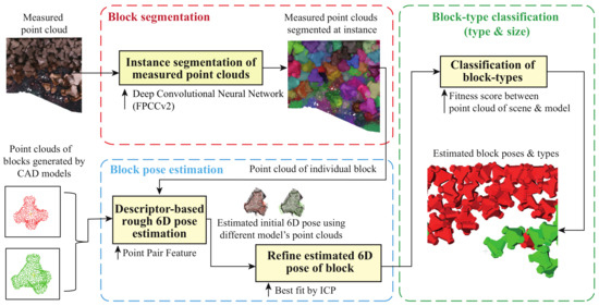
Figure 2.
Pipeline of block detection. The algorithm consists of three steps for detecting the type and 6D pose of all block instances in the scene. The input is the point cloud of a scene measured by the UAV or MBES. The point cloud of an individual block is output by convolutional network FPCCv2 (Block segmentation). Next, 6D poses for multiple models were roughly estimated by PPF and refined by ICP (Block pose estimation). Finally, the block type is determined based on the fitness score (Block-type classification).
- First, the category-agnostic instance segmentation network FPCCv2 segments the input point cloud measured by UAV and MBES into the subsets of points corresponding to individual block instances. FPCCv2 is a kind of deep neural network, which is pre-trained by synthetic point clouds that mimic the point clouds of stacked blocks measured by UAV and MBES, respectively, using the stacked block CAD models and surface point sampling. The detailed algorithms are described in Section 4.
- Second, the 6D pose of an individual block is estimated from each segmented point cloud using a conventional descriptor-based 3D object detection algorithm that makes use of PPF [15] and ICP [16]. The detailed algorithm is described in Section 5.1.
- Finally, if the scene consists of multiple typed blocks, a fitness score corresponding to each type is calculated for each segmented point cloud to identify the type of detected individual block. The detailed algorithm is shown in Section 5.2.
4. Instance Segmentation of Measured Point Cloud Based on Deep Neural Network
The first and crucial step of our wave-dissipating block pose detection is an instance segmentation of an original point cloud using a deep neural network. The category-independent instance segmentation network, called FPCCv2, segments input point clouds measured by UAV and MBES into subsets of points corresponding to individual blocks. FPCCv2 is an extended version of our previous instance segmentation network FPCC [14] with a novel feature extractor. Therefore, this section first revisits FPCC; then, it explains why we must improve our previous FPCC to address the issue of instance segmentation of wave-dissipating blocks and how we improved it to solve the issue.
4.1. FPCC and Its Limitation
FPCC was originally developed by Xu et al. [14] as a category-agnostic 3D instance segmentation network for discriminating each part in an industrial bin-picking scene in robotic automation, where the parts have an identical shape and overlap each other. FPCC extracts features of each point, while inferring the centroid of each instance. Subsequently, the remaining points are clustered to the closest centroids in the feature embedding space. It was shown that even FPCC trained by synthetic data performs at an acceptable level on real-world data [14].
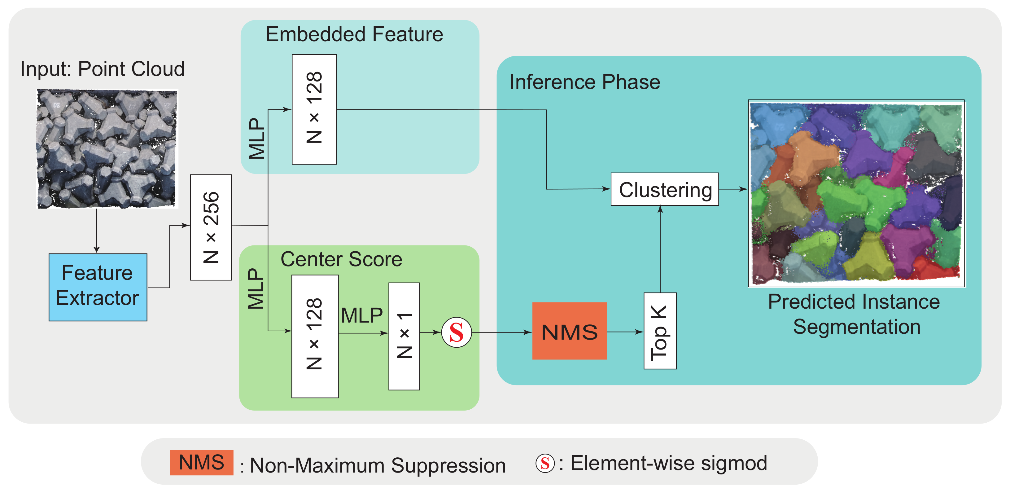
As shown in Figure 3, FPCC is composed of a point-wise feature extractor and two branches: an embedded feature branch and a center score branch. The point-wise feature extractor has the same semantic segmentation structure as DGCNN [50]. The extracted features are sent to the point-wise embedded feature branch and center score branch, respectively. The instance segmentation can be regarded as a kind of point cloud clustering, and the clustering method of FPCC assumes that the points in the same instance have similar features, while points in the different instances have relatively different features. In contrast, the center score branch predicts the probability of each point to be placed at the centroid. In the prediction phase, non-maximum suppression finds the point with the highest score for each target object as a reference point for clustering. Then, the distances between the remaining points and the reference point were calculated. Finally, the remaining points are clustered into the same instance with the center point by feature distance.
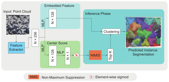
Figure 3.
Network architecture of FPCC [14]. After the Center Score branch predicts the probability that each point is likely to be the centroid of the object, non-maximum suppression is used to select the most likely centroids as reference points for clustering. The reference and remaining points are clustered according to the L2 distance in feature space. Our improvement aimed for FPCCv2 is the feature extractor (Section 4.2), where the features of point clouds can be exploited more effectively than the original FPCC.
Although FPCC exhibits a promising instance segmentation performance in robotic bin-picking [14,27,41,51], a computational and efficiency issue could arise when applying it to the instance segmentation of large-scale point clouds captured from stacked wave-dissipating blocks in real breakwaters.
FPCC made use of DGCNN [50] as the feature extractor. DGCNN employs the k-nearest neighbor (k-NN) algorithm to construct the graph of the point cloud in three-dimensional space and high-dimensional space, such that the topological structure of the graph of DGCNN is not static but dynamically updated after each layer of the network. Dynamically updating the graph can heavily increase training and prediction time and limits the number of points that the network can process per frame under the same memory size. To encode the features of large-scale point clouds faster and better, a novel feature extractor is added to the original FPCC. Details are described in the next section.
4.2. Proposed Feature Extractor for FPCCv2
To solve the issue pointed out in Section 4.1, as shown in Figure 4, the feature extractor of FPCCv2 consists of three parts: (1) dilated graph convolutions (GraphConv), (2) relative local information, and (3) attentive pooling.

Figure 4.
Feature extractor of FPCCv2 is built from a sequence of graph convolutions and MLPs. The high-dimensional (e.g., 512) features of each point are fed into the center score branch and the embedded feature branch of the original FPCC network, respectively.
Dilated Graph Convolution. Our goal was to give each point reasonable and sufficient information within an acceptable computational overhead. Previous studies [52,53,54] showed that the size of the receptive field is essential to the performance of a network. A larger receptive field can offer neural units more comprehensive and higher dimensional features. However, a too-large receptive field makes it more difficult for the network to learn high-frequency or local features [54]. Stacking convolutional layers or increasing the kernel size of convolution are common approaches to increase the receptive field.
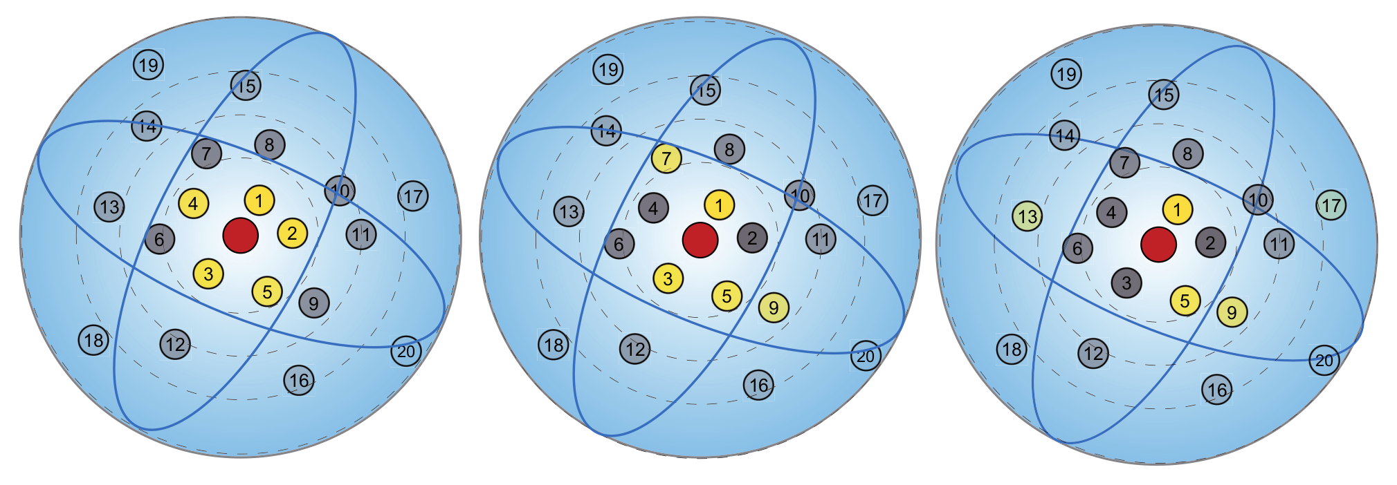
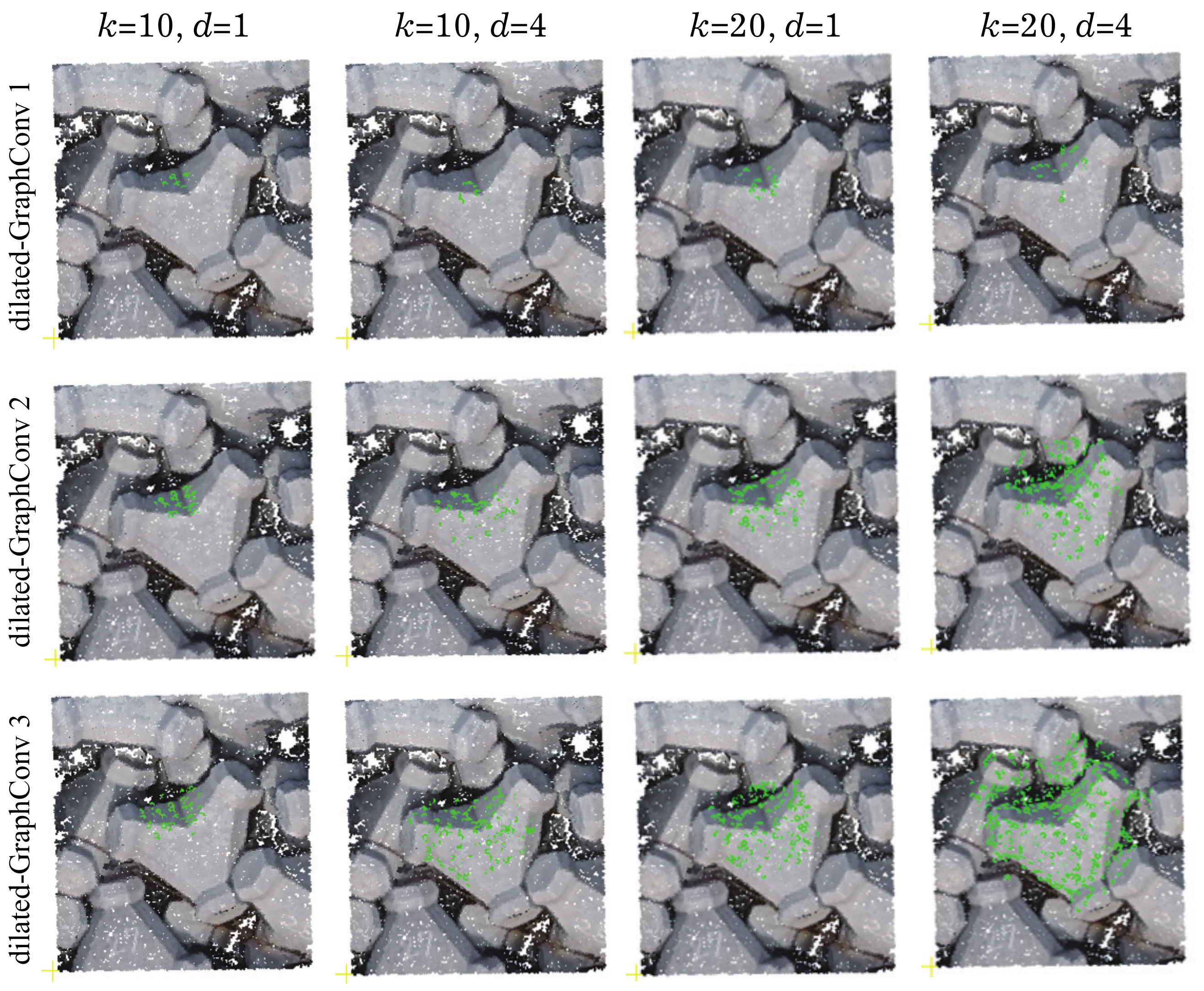
Inspired by previous research [52,54], the dilated local graph is defined by a dilated K-NN in Euclidean space. The d-dilated K-NN first finds nearest neighbors for a point i but only selects every d points from the nearest as the neighbor point set (see Figure 5). Therefore, some computational overheads are increased to expand the receptive field without increasing the number of model parameters. Three dilated graph convolutions were stacked in our feature extractor. The receptive field sizes with different k and d after each dilated graph convolution are shown in Figure 6. Then, the relative feature of a point i to point k in its corresponding d-dilated K-NN neighbor points is defined as:
where and are, respectively, the feature of point i and k for . In the first graph convolution, f is selected as x-y-z coordinates of the point. represents a multilayer perceptron. Figure 7 illustrates the process of the dilated graph convolution.
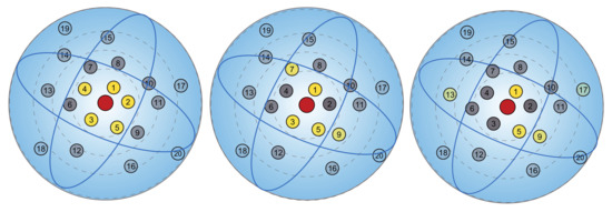
Figure 5.
Nearest neighbor selection of dilated k-NN [52]. The number in the circle represents the distance from center point (red). k-NN, where , with different dilation rates 1, 2 and 4 (left to right) selecting different points (yellow) as relative points.
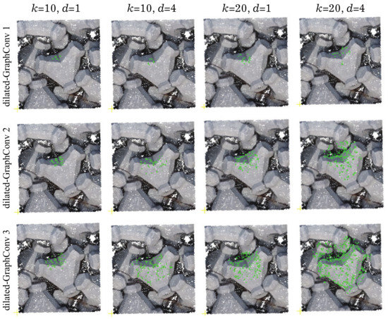
Figure 6.
Visualization of the receptive field. The receptive field (green point) expands with deeper networks (rows). Increasing nearest neighbors k and dilation rate d can enhance the receptive field with less computational overhead. When , the receptive field of the third layer can roughly cover a complete block.

Figure 7.
Dilated Graph Convolution. N points are input and K relative features of each point are output.
Relative Local Information. The relative local information of a point i with its d-dilated K neighbor points is defined as:
where and denote three-dimensional coordinates of point i and k for , ⊕ represents the concatenation operation, and denotes Euclidean distance between the two points. The relative local information of each point is repeatedly introduced into the network to learn local features efficiently.
Attentive Pooling. Given a set of features , where and M denotes the size of pooling. Attentive pooling aims to integrate F into a single feature while achieving permutation invariance of its elements. The existing methods [50,55,56] use simple max/mean pooling to address the permutation invariance, resulting in the loss of crucial information [57]. Influenced by recent studies [57,58], we employed attentive pooling in aggregating relative features, as shown in Figure 8. The attentive pooling operation consisted of the following steps:

Figure 8.
Attentive pooling. K by a-dimensional relative features of N points are integrated in this module with the permutation invariance.
(1) Association with location information. For each point i, the relative features and relative local information of the d-dilated K-NN neighbor points were concatenated to generate a new feature . The new feature set is defined as .
(2) The feature set is fed into a shared to obtain initial attention scores , where has the same dimension as , and it is defined as:
(3) A softmax normalizes the elements of to obtain the attention score . The attention score is defined as:
where
where , are the d-the elements of , . The learned attention score can actively discriminate the degree of importance among features around a point. Finally, the weighted summed feature of a point i is given by:
where ⊗ represents element-wise multiplication.
A sequence of Dilated Graph Convolution and Attentive Pooling modules are stacked in the feature extractor. Theoretically, the more modules that are stacked, the larger the receptive field of each point will be. However, more modules would inevitably sacrifice the overall computational efficiency, and an excessively large receptive field is unnecessary [57]. The features integrated by the three Attentive Poolings were fed into three MLPs and then concatenated. Finally, these features were fed into two MLPs with a skip connection. Following the structure of the original FPCC, the 512-dimensional features of each point were extracted and fed into the two branches of the FPCC.
4.3. Generation of Data for Instance Segmentation
As discussed in Section 2.2, creating a rich and reliable training dataset is essential for instance segmentation of measured point clouds of wave-dissipating blocks based on deep learning. However, creating this training dataset by manually labeling block instances in large-scale real measured point clouds is labor intensive and practically impossible. To address this issue, the FPCCv2 is only trained by synthetic point cloud data that mimics the stacking poses of wave-dissipating blocks and evaluated on real-world and synthetic data.
Several previous studies [59,60,61] used synthetic images to train the network through domain randomization. These methods proved successful through sophisticated image rendering. However, the color of blocks in outdoor environments can change due to uncontrollable factors, such as seawater, light and season, etc. Synthetic data face difficulty covering these influences. Based on this consideration, RGB information of the point cloud was not used in training and prediction. There are at least two advantages to this approach. The first is that the data are easier to synthesize in an acceptable period without manual work. The second is that it makes the network more robust and avoids interference of environmental factors.
The following procedure generates our synthetic point cloud data of the stacked wave-dissipating blocks.
- A triangular mesh model of a wave-dissipating block is created from the surface tessellation of its 3D CAD model.
- Subsequently, a point set is densely sampled on every triangle face of the mesh model .
- A variety of penetration-free stacking poses of piled blocks are generated using a set of triangular mesh model instances for the model . Furthermore, a set of sampled points on blocks in stacking poses is calculated for each block as on the model instances , respectively.
- A subset of the sample points on the block model in the stacking poses is picked up as that are only visible from a given position of the measurement device.
- For every point , Gaussian noise at a certain level is imposed on the coordinates of q, which simulates the possible accidental error induced from the measurement device to create the final synthetic point cloud. The point cloud is used to train our instance segmentation network (FPCCv2).
Figure 9 shows the examples of triangular mesh models of wave-dissipating blocks used for generating the synthetic point cloud data used in this study.

Figure 9.
Triangular mesh models of wave-dissipating blocks are used in this study. We named these blocks Block A1 (a), Block A2 (b), Block A3 (c), Block B1 (d) and Block B2 (e). They are made of concrete to dissipate the force of waves. Notably, A1, A2, and A3 have the same shape but different sizes, and so do B1 and B2.
The stacking of blocks is simulated in the Bullet physics engine [17]. As shown in Figure 10, the penetration-free block-stacking scene under gravitation can be reconstructed in real time. About 50 identical blocks are stacked in a square with a side length about five times the maximum length of the block in a computer.

Figure 10.
Synthetic point cloud of stacking poses of piled blocks. (a) Original set of sampled points on blocks in stacking poses . Point clouds of different block instances are rendered in different colors. (b) Point cloud after removing invisible points and adding artificial Gaussian noise that mimics the measurement error.
Figure 10 illustrates the generation procedures of synthetic point cloud data. The position of the measurement devices is defined corresponding to the UAV-mounted camera and sonar of the MBES, as shown in Figure 10a. Figure 10b illustrates use of the hidden-point removal algorithm [62] to eliminate the invisible sample points on the block model from the original set of sampled points on the blocks to obtain the visible sample points . Considering the noise levels of UAV and MBES that were found in the preliminary experiment, we added Gaussian noise with a standard deviation of 1 mm to the sampled point cloud measured from the UAV-mounted camera, and a standard deviation of 3 mm to that from the MBES sonar.
We generated six groups of the synthetic point cloud data corresponding to the UAV and MEBS measurements of the blocks in three ports, each containing 500 training and 100 test point clouds. The generation for one synthetic point cloud took about three minutes in a standard desktop PC.
5. Block Pose Estimation and Type Classification
After segmenting the input point cloud into a set of points corresponding to individual block instances, the 6D pose of an individual block is estimated from each segmented point cloud using the PPF descriptor [15] and the best-fit point cloud alignment by ICP [16]. Moreover, the block-type is classified based on the pose estimation results. The detailed algorithm is described in this section.
5.1. Block 6D Pose Estimation Using 3D Feature Descriptor
First, a brief introduction to the PPF [15] descriptors for pose estimation is given. Owing to the powerful instance segmentation of FPCCv2 of the original point clouds, the input original measured point cloud Q has already been partitioned into a set of instance point clouds , where denotes the point cloud corresponding to the potential surface of an individual block l. Therefore, the original PPF algorithm is sufficient to estimate the 6D pose of an individual block l from a given point cloud .
PPF-based pose estimation combines a hash table and a voting scheme for matching the point cloud of a 3D object model to the one of 3D scenes to estimate the 6D pose of an object.
The PPF descriptor for a pair of 3D points in a point cloud corresponding to the block l is defined as a four-dimensional vector by
where denotes the normal vector at a point , , where denotes a coordinates of point i, and denotes the angle between a vector and , as shown in Figure 11. descriptors are generated from every pair of points in the point cloud and stored in a hash table, where is used for the hash key. Because the PPF descriptor is defined only by a distance and angles between a pair of points, it is invariant to the rotation and translation.
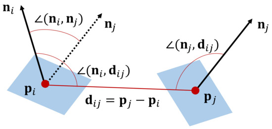
Figure 11.
Illustration of Point Pair Feature (PPF).
A point cloud corresponding to an instance point cloud in a scene is sampled to approximately the same resolution as the sampled point cloud on a mesh model . After sampling, given a scene point pair , the model point pair that shares a similar PPF descriptor value to can be retrieved using the hash table. To match the two point pairs, first, the point pairs and are transformed by the homogeneous transformation matrix and , respectively, such that and move to the origin, and their normals are aligned to the .
Then, the rotation matrix that rotates by an angle around the x-axis is found, such that matches to . These transformations can be defined as Equation (8):
where and denote the 3D coordinates of the point and , respectively.
Finally, in the voting scheme, for a given reference scene point , PPF is evaluated with all other scene points , after which it is matched with those of all point pairs on the model using the hash table. For each potential match, one vote is cast in a 2D accumulator . After all matches are completed, the candidate poses over the threshold vote number are selected for clustering. The score of a cluster is the number of the candidate poses it contains, and the cluster with the highest score yields the estimate of the block pose. Finally, according to Equation (8), the pose of a block l is estimated as
where denotes the rotation matrix, and denotes the translation of a block l.
5.2. Pose Refinement and Block-Type Classification
Some breakwaters are armored with two or more types of blocks, so it is necessary to register the point clouds of different types of block models with segmented scene point clouds. First, the poses roughly estimated by PPF are refined by ICP; subsequently, the fitness score is evaluated. The fitness score represents the relative distance between the segmented scene point cloud of a block l and registered model point cloud , where u indicates the type of the block.
The fitness score B is the average minimum Euclidean distance between the point clouds of and , and it is defined as Equation (10):
where is the i-th point in the point cloud , is the j-th point of the model point cloud . The score B reflects how accurately the two point clouds match, where a lower score is better. Among different block types U, with the smallest fitness score B is determined as the most likely one.
6. Results of Wave-Dissipating Block Detection
6.1. Experimental Sites
Three breakwaters at Sawara port, Todohokke Port, and Era Port in Hokkaido prefecture, Japan, were used for evaluation of the proposed block detection algorithm. For these ports, existing block point clouds above the water surface were measured by UAV and a commercial photogrammetry software, and those below the surface were measured by MBES. Table 1 indicates the details of the data of these sites, and Figure A1 shows the top view of the point clouds.

Table 1.
Detail of point cloud data of three ports.
Only one type of block was used for the Sawara port, and two different types of blocks were used for the Todohokke and Era ports. Because the point cloud of all ports contains more than a million points, the proposed algorithm cannot handle it at once due to the memory limitation. Therefore, the original point cloud of the whole site was partitioned into several regions (10 to 25 meters by 10 to 25 meters) to test the proposed block detection method, as shown in Table 1. Depending on the extent of the construction, the length and width of each region is approximately five times the size of the corresponding block, and the areas range approximately 100 to 600 .
6.2. Block Instance Segmentation
6.2.1. Experimental Setting of CNN
Our block instance segmentation network FPCCv2 was implemented in the TensorFlow framework and trained using the Adam optimizer with an initial learning rate of 0.0001, batch size of 1, and momentum of 0.9. The network was trained for 60 epochs. It took approximately 30 h to train FPCCv2 for each block-stacking scene. All training and testing are performed on an NVIDIA GeForce RTX 2080 Ti GPU and an Intel Core i9-9900k CPU with 64 GB of memory. The training data is an all synthetic point cloud, as described in Section 4.3.
6.2.2. Precision and Recall
The performance of the block instance segmentation by FPCCv2 is evaluated on real UAV data and synthetic MBES data. Blocks of the same type but different sizes were stacked in Todohokke port and Era port. Because FPCCv2 is a category-agnostic clustering algorithm, differences in their size are not classified in this stage but in the block classification stage described in Section 5.2.
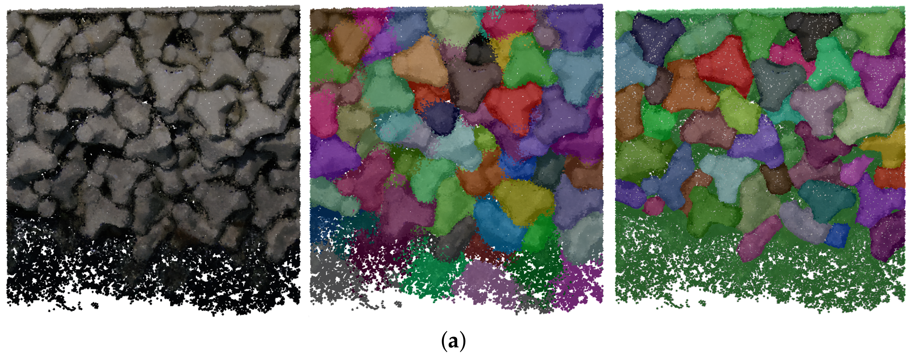
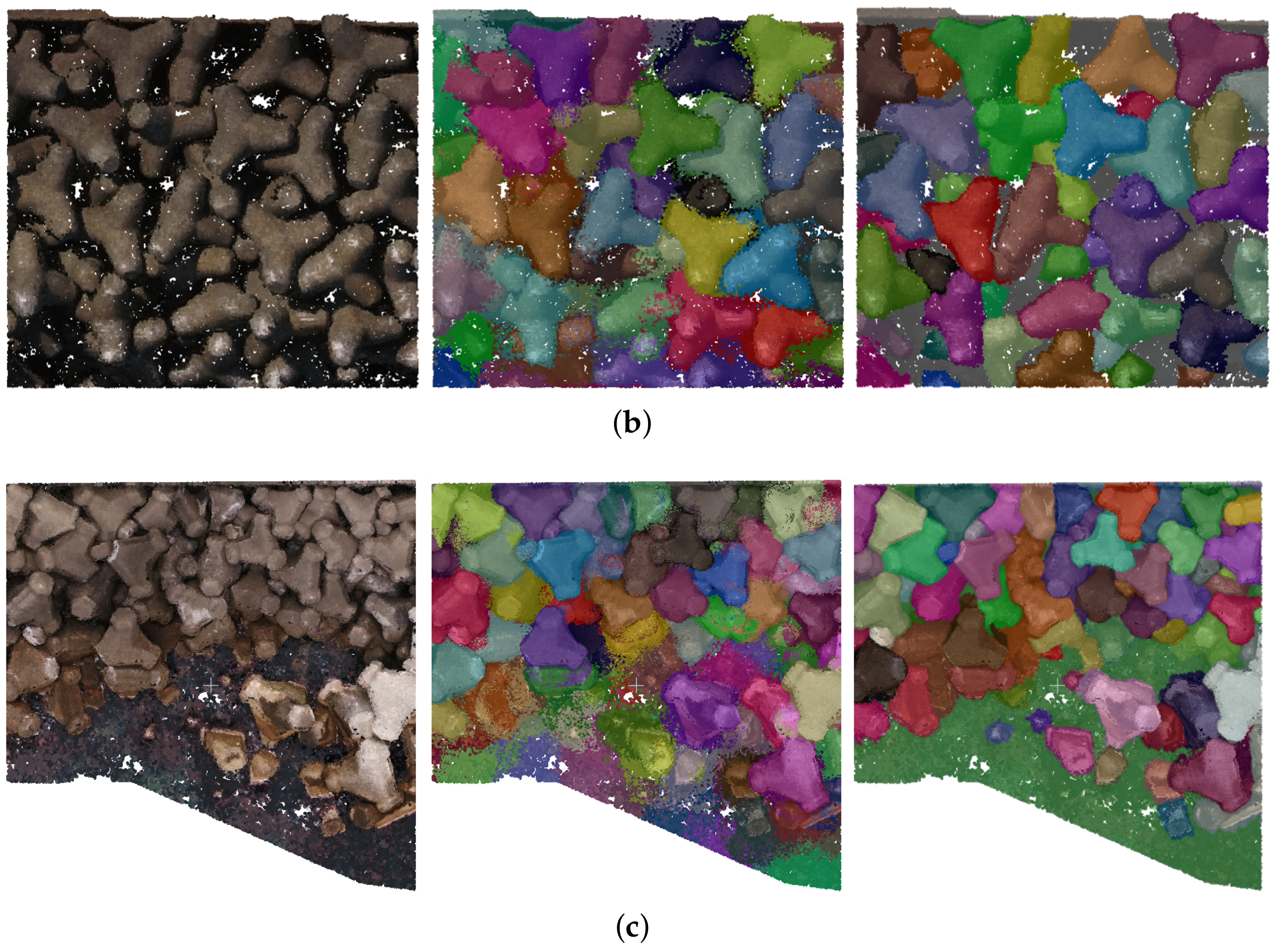
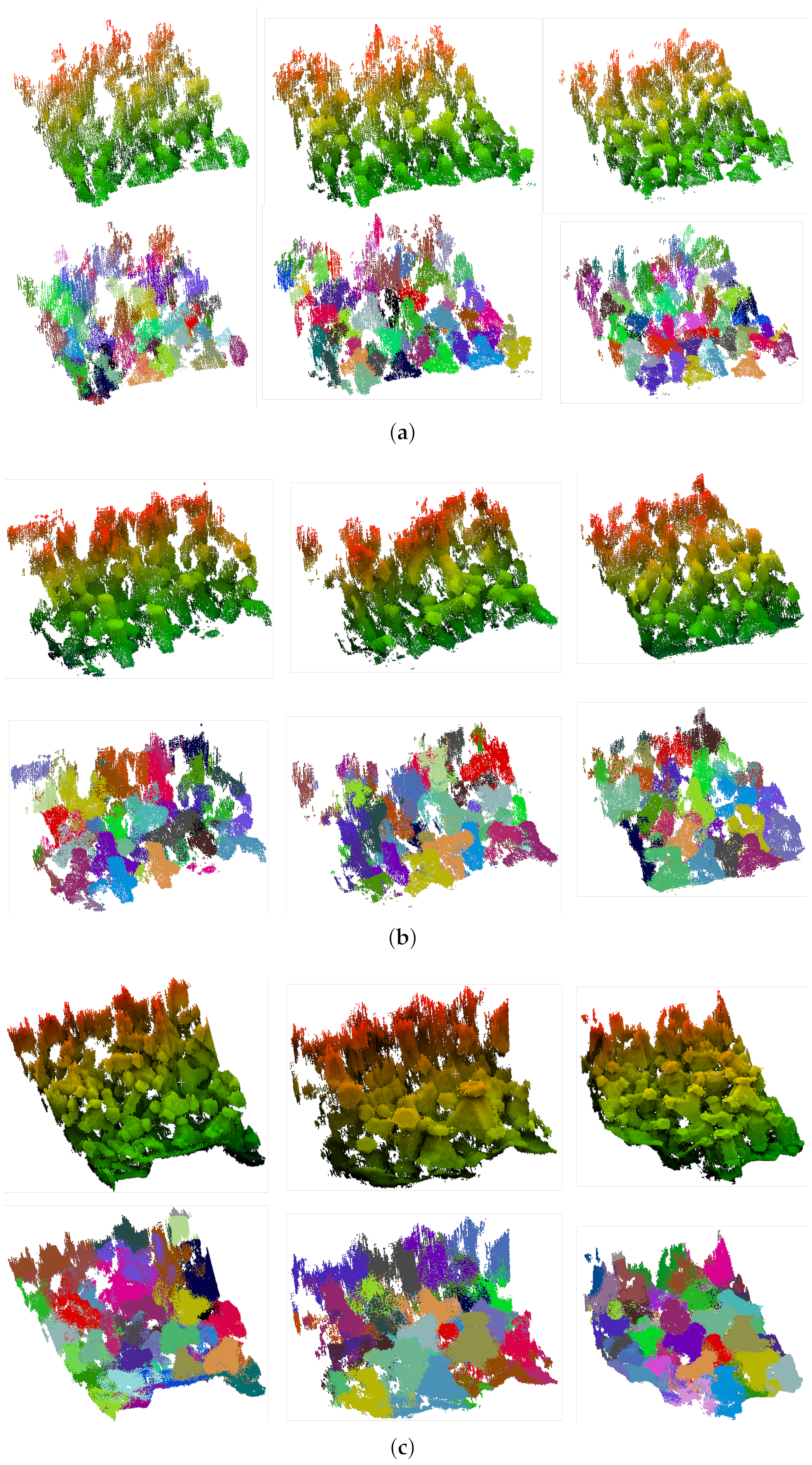
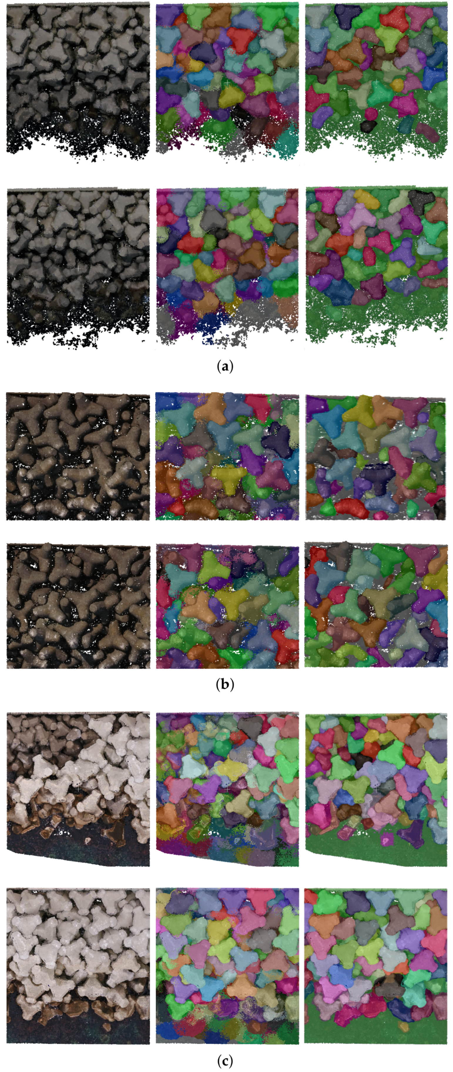
Figure 12 and Figure 13 illustrate the results of the block instance segmentation predicted by FPCCv2, and further results are shown in Figure A2. Different blocks are rendered by different colors. While there are some blurs at the boundary of neighboring blocks, Figure 12 and Figure 13 show that the main body of each block could be clearly segmented.
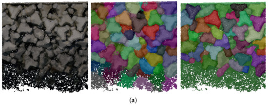
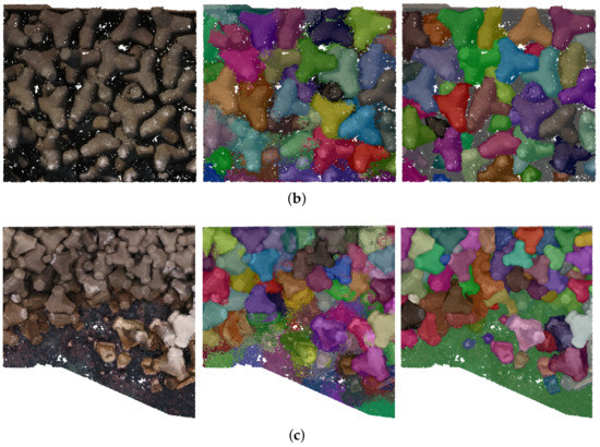
Figure 12.
Instance segmentation results on Sawara port (a), Todohokke port, (b) and Era port (c). The left column is the point cloud scene measured by UAV. The middle column is the predicted result of instance segmentation, and the last column is the ground truth. Different colors represent different blocks.
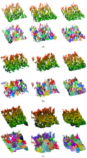
Figure 13.
Visualization of instance segmentation results on MBES data. The first row of Sawara port (a), Todohokke port (b) and Era port (c) is the original point cloud measured by MBES. The second row of each subfigure is the predicted results of instance segmentation. Different colors represent different blocks.
However, the segmentation of the area near sea surface is poor, because the original points measured in this area are noisier due to wave splash.
Table 2 summarizes the block-wise precision and recall of the instance segmentation with an intersection of union (IoU) threshold of 0.5. The ground truth instance label of the UAV test regions is made manually by referring the orthorectified image of these sites. The MBES test data used for quantitative evaluation are synthetic, because MBES data are noisy, and the boundaries of the objects are blurred, making it difficult to label them manually. The precision on UAV data reached over 80%, while the recall rate ranges between 50 and 76%. The recall on the real UAV data is lower than that on the synthetic MBES data. We attribute this to some extremely small visible part of blocks in the real scene, which are difficult to be retrieved and segmented.

Table 2.
Performance of instance segmentation on blocks in three ports. Metrics are precision (%) and recall (%) with an IoU threshold of 0.5. The UAV point cloud was measured from real-world scenes, and ground truth segmentation was performed manually, while the MEBS point cloud was synthesized.
6.3. Block Pose Estimation
6.3.1. Synthetic Data Set Creation
Because manually labeling the 6D poses of all blocks included in a real point cloud scene of wave-dissipating blocks is a time-consuming and ambiguous task, the accuracy of block pose estimation is evaluated on six sets of synthetic datasets mimicking the UAV and MBES point clouds from the three ports. Each set contains 100 scenes with pose annotation. Figure 14a shows examples of the synthetic dataset.
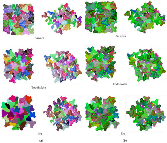
Figure 14.
(a): Synthetic point clouds for three ports. (b): Pose estimation results on synthetic point clouds. Block models are transformed to the scene using estimated poses.
6.3.2. Pose Estimation Accuracy Using Synthetic Data Set
A pose of a rigid 3D object is generally represented by a matrix , where is a rotation matrix and is a 3D translation vector. Because numerous wave-dissipating block shapes exhibit a certain number of geometric symmetries, and these symmetric poses are equivalent in appearance, the accuracy of block pose estimation must be evaluated by considering these equivalent poses.
Taking the symmetry of a block geometry into account, a set of equivalent symmetric poses of the block can be represented by its ground truth 6D pose , where and , as shown in Equation (11).
where is the group of equivalent symmetries that have no effect on the static state of an object [63]. Based on Equation (11), the displacement error and rotation error between an estimated pose and its ground truth pose are evaluated by
and
The largest edge size of the bounding box of a block is set to ; if the displacement error is within and the rotation error is within , the case was counted as a true positive; otherwise, it was considered as a false positive. Herein, performance metrices, precision and recall, evaluated the case where a scene contains numerous blocks, and the average precision and recall of all scenes in each port were finally calculated. Only blocks with a lower than 80% occlusion rate are considered of interest to retrieve. Following the work [64], the occlusion rate is defined as:
Table 3 presents the accuracy of pose estimation for each port, and Table 4 offers the displacement and rotation errors. Our method performs well on synthetic data, not only retrieving roughly 80% of blocks but also with the errors less than 40 mm and in the pose estimation. Figure 14b yields some visualization of the pose estimation results on synthetic data.

Table 3.
Block-wise accuracy of block pose estimation for synthetic scenes. Only blocks with a <80% occlusion rate are considered of interest to retrieve. The metrics are precision (%) and recall (%) with a displacement error and rotation error .

Table 4.
Average of displacement and rotation errors for synthetic scenes. : displacement error (mm); : rotation error ().
6.3.3. Pose Estimation Accuracy Using Real Scene Data
It is practically difficult to prepare the ground truth poses of stacked individual blocks in a real scene. Therefore, in this study, the difference between the block surface with estimated poses and original point cloud indirectly indicates the accuracy of block pose estimation in real scenes.
To this end, we employed two indirect evaluation metrics: the average fitting error and the matching rate. As shown in Figure 15, for every point i in a scene point cloud, the distance from i to the closest face on the block CAD model that fits to the point cloud is examined first. Then, the average fitting error is calculated as:
where is the threshold distance for the accuracy evaluation.

Figure 15.
Average fitting error for block pose estimation.
Another metric, matching rate R, is used to indirectly evaluate the recall of pose estimates, which is defined as:
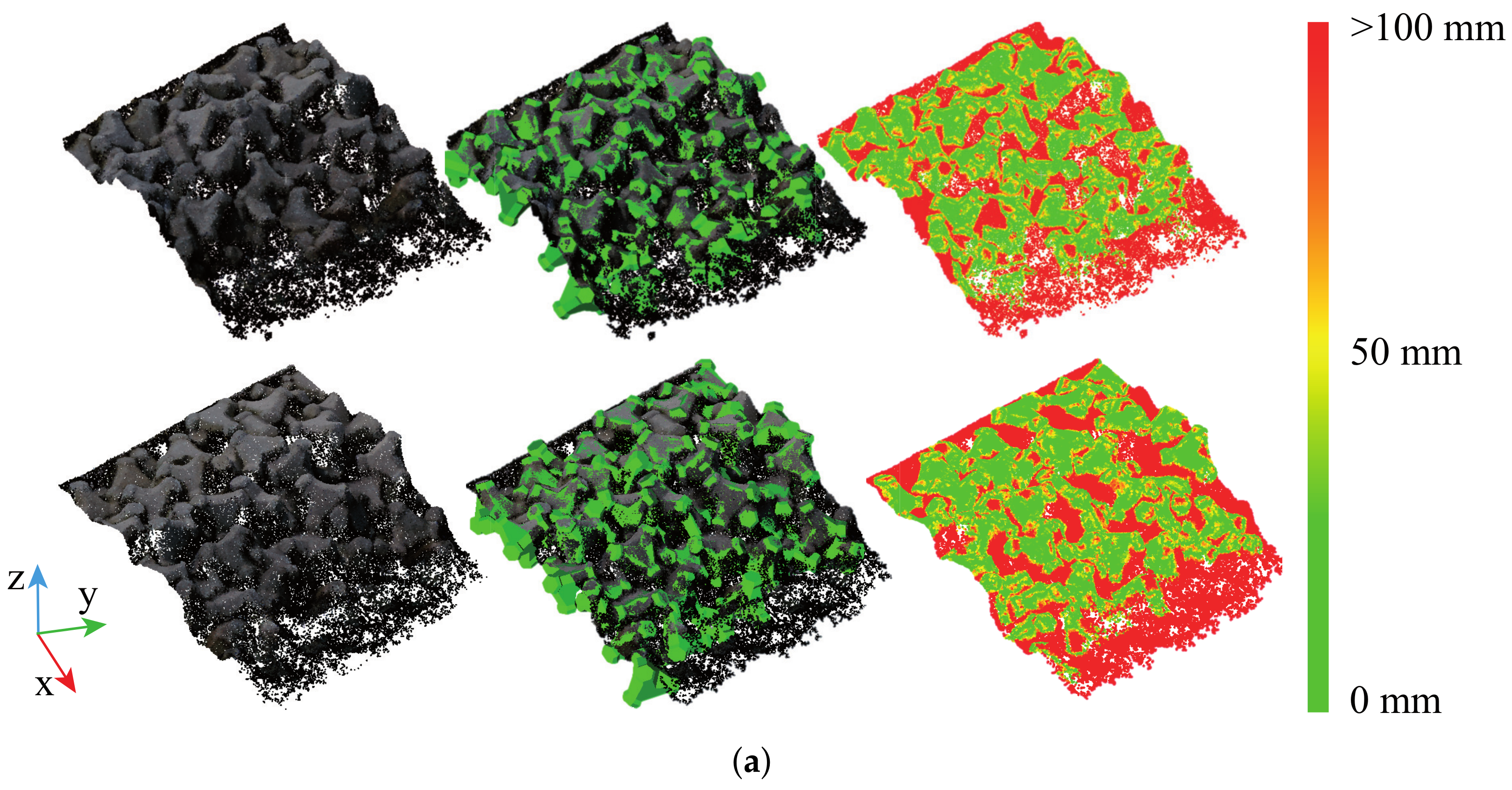
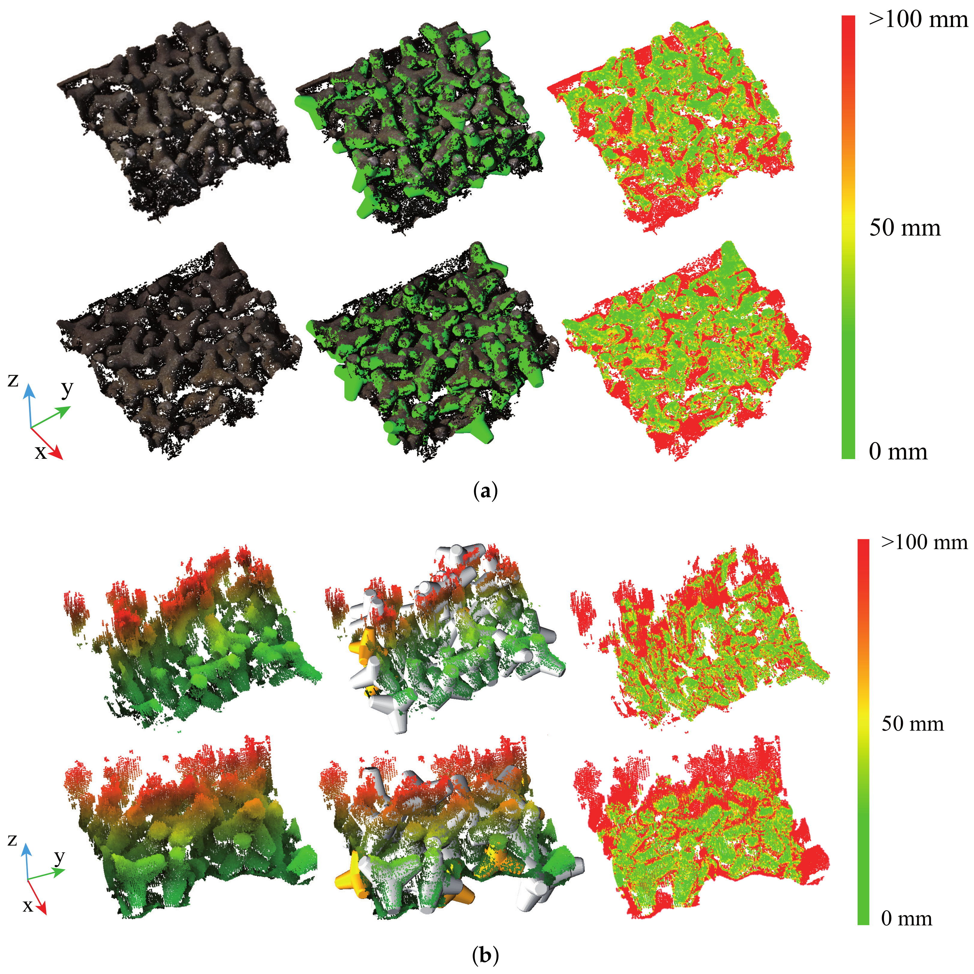
Examples of the average fitting error and matching rate are visualized in Figure 16 and Figure 17. The average fitting error and matching rate of UAV and MBES data for the three ports are summarized in Table 5. The results on real data show that our method can match more than 60% of the points with a small pose estimation error, and almost all visible blocks in a scene can be retrieved. Meanwhile, the measured boundary of the MEBS point cloud decreases the performance of the method due to the excessive noise.

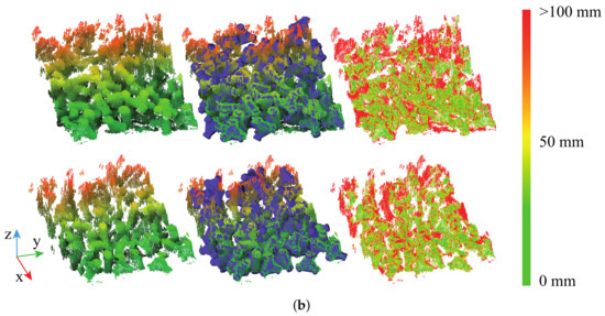
Figure 16.
Visualization of pose estimation on UAV data (a) and MBES data (b) of Sawara port. The first column is the measured point cloud. The block models are transformed to the scene space using pose results and displayed in the middle column. The last column is a visualization of the average fitting error of the pose estimates, where the red points indicate that its distance from the nearest block model is larger than 100 mm.

Figure 17.
Visualization of pose estimation on UAV data (a) and MBES data (b) of Todohokke port. The first column is the measured point cloud. The block models are transformed to the scene space using pose results and displayed in the middle column. The last column is a visualization of the average fitting error of the pose estimates, where red points indicate that its distance from the nearest block model is larger than 100 mm.

Table 5.
Accuracy of pose estimation for various blocks in real scenes. : fitting error (mm); R: matching rate (%). m for Sawara and Todohokke, m for Era.
6.4. Block-Type Classification
Finally, the performance of our multiple block-type classification was evaluated on the UAV point cloud from the Todohokke and Era ports. As described in Section 5.2, after estimating the pose of a block, fitness scores were calculated using different model point clouds of blocks and corresponding scene point clouds. The one with the smallest fitness score was regarded as the correct block type. The ground truth of the block type was determined by taking manual size measurement for the points sampled from the original scene point cloud and comparing the size with the standard block size specification disclosed in advance from its manufacturer.
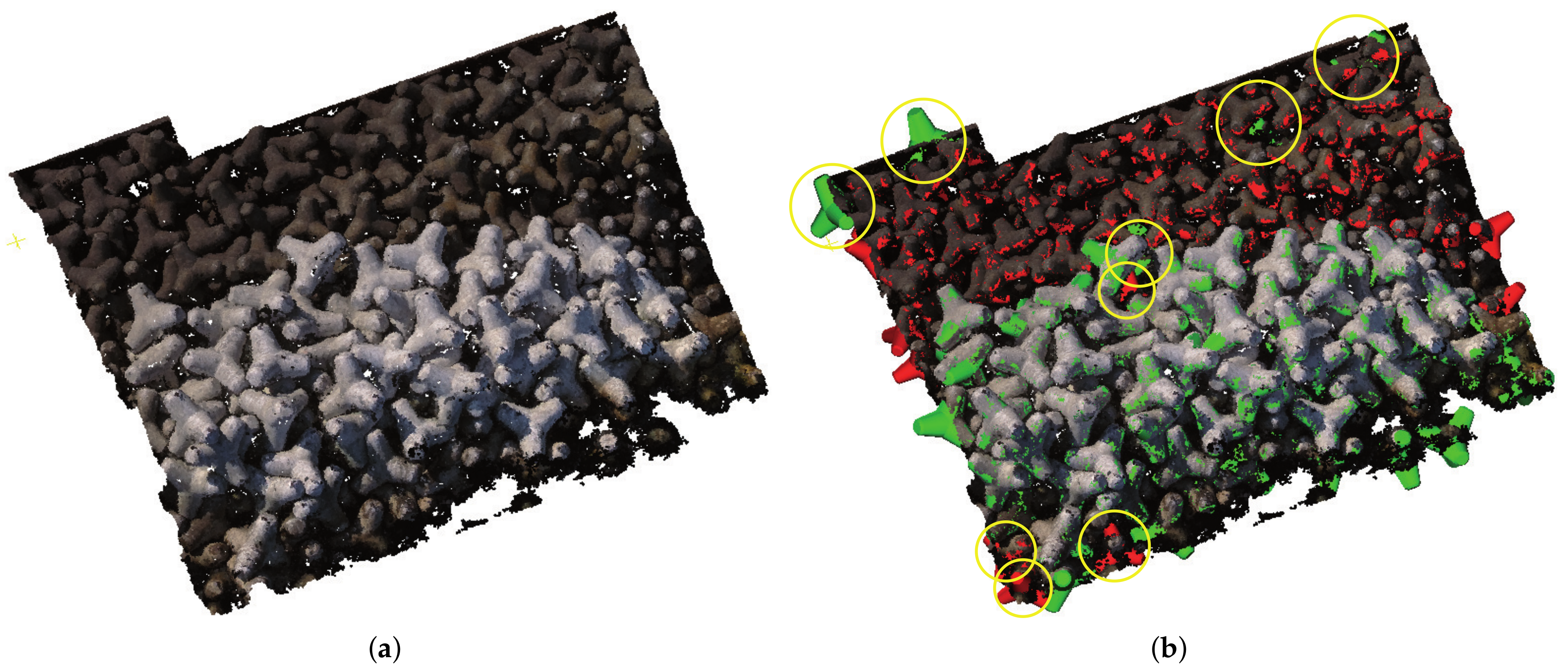
The block-type classification performance is indicated in Table 6. Figure 18 presents the block-type classification result for the Todohokke port, where a total of 135 blocks were recognized, of which nine misclassifications are indicated by yellow circles. The block-wise accuracy reached 94%. Figure 19 shows the result of block-type classification of the Era port, where a total of 181 blocks were recognized, of which six misclassifications are indicated by yellow circles. The accuracy rate reached 96%. As shown in Figure 18, the incorrect results occur mainly at the boundaries of the data, where the points of the blocks are incomplete, and in the part near the sea, where the noise is relatively high.

Table 6.
Accuracy of block-type classification.
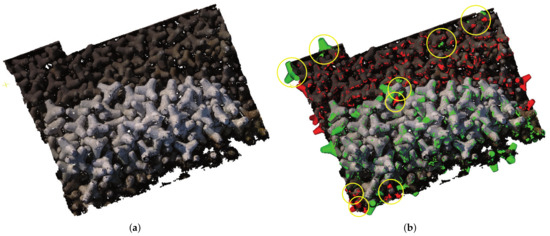
Figure 18.
Visualization of results of block-type classification on Todohokke port. (a) is the real point cloud scene of Todohokke port measured by UAV, and (b) is the result of type classification after instances segmentation and pose estimation. Block B1 and Block B2 are rendered in red and green, respectively. The yellow circles indicate misclassified blocks.
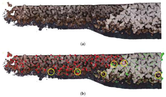
Figure 19.
Visualization of results of block-type classification on Era port. (a) is the real point cloud scene of the Era port measured by UAV, and (b) is the result of type classification after instances segmentation and pose estimation. Block A2 and Block A3 are rendered in red and green, respectively. Yellow circles indicate misclassified blocks.
6.5. Processing Time
This section provides the processing time for each step in our method. Table 7 presents the processing time for synthetic training data creation and the training of our instance segmentation network (FPCCv2). Five hundred artificial point cloud scenes of piled blocks shown in Figure 10 that mimic UAV and MBES measurements were used to train FPCCv2 with an epoch of 60. Approximately 30 h of training were required in each UAV or MEBS data.

Table 7.
Processing time for synthetic training data creation and instance segmentation network training.
Table 8 summarizes the computation time for block detection, except training. Once learned, the FPCCv2 could segment about 100,000 points into block instances in less than 1 s and 700,000 points in about 4 s. Pose estimation time was about 3 min per region. On average, each region of Sawara and Era included 40 blocks and each region of Todohokke contained 30 blocks. Time taken for block classification was about 30 s per region for Sawara and Todohokke and about 2.5 min per region for Era.

Table 8.
Processing time for block detection.
These results show that the proposed block detection method is sufficiently fast for practical use.
7. Conclusions
A novel deep-learning-based approach to detect individual blocks from large-scale three-dimensional point clouds measured from a pile of wave-dissipating blocks placed overseas and underseas using UAV-photogrammetry and MBES was proposed. The approach consisted of three main steps. First, the instance segmentation using our originally designed deep convolutional-neural network (FPCCv2) partitioned an original point cloud into small subsets of points, each corresponding to an individual block. A physics engine enabled generating instance-labeled training datasets synthetically and automatically for the instance segmentation of blocks, avoiding laborious manual labeling work and secure rich training datasets for our convolutional-neural network. Subsequently, the block-wise 6D pose was estimated using a three-dimensional feature descriptor (PPF), point cloud registration (ICP), and CAD models of blocks. Finally, the type of each segmented block was identified using the model registration results.
The results of the instance segmentation on real-world and synthetic point cloud data achieved 70–90% precision and 50–76% recall with an IoU threshold of 0.5. The pose estimation results on synthetic data achieved 83–95% precision and 77–95% recall under strict pose criteria. The average block-wise displacement error was 30 mm, and the rotation error was less than . The pose estimation results on real-world data showed that the fitting error between the reconstructed scene and the scene point cloud ranged between 30 and 50 mm, below 2% of the block size detected. The accuracy in the block-type classification on real-world point clouds reached approximately 95%. These block detection performances proved the effectiveness of our approach.
In future studies, we plan to reconstruct the virtual scene of current wave-dissipating blocks in the physics engine based on our detected block poses and then simulate and generate a more accurate construction process plan of block supplemental work than the conventional one according to practical requirements. This would guide the accuracy, save construction time, and visualize the construction process and results.
Author Contributions
Conceptualization, Y.X. and S.K.; methodology, Y.X. and S.K.; software, Y.X.; validation, Y.X.; formal analysis, Y.X.; investigation, Y.X.; resources, Y.X., S.K., H.D. and T.S.; data curation, Y.X., S.K. and H.D.; writing—original draft preparation, Y.X. and S.K.; writing—review and editing, Y.X. and S.K.; visualization, Y.X.; supervision, S.K. and H.D.; project administration, S.K.; funding acquisition, S.K. and T.S. All authors have read and agreed to the published version of the manuscript.
Funding
This work was supported by JST SPRING, Grant Number JPMJSP2119.
Data Availability Statement
Our code for block instance segmentaion is available at https://github.com/xyjbaal/wave-dissipating-seg.
Conflicts of Interest
The authors declare no conflict of interest.
Appendix A
Some relevant figures are provided in this section.
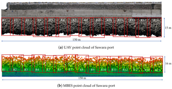
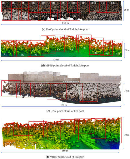
Figure A1.
Point cloud of three ports.
Figure A1.
Point cloud of three ports.
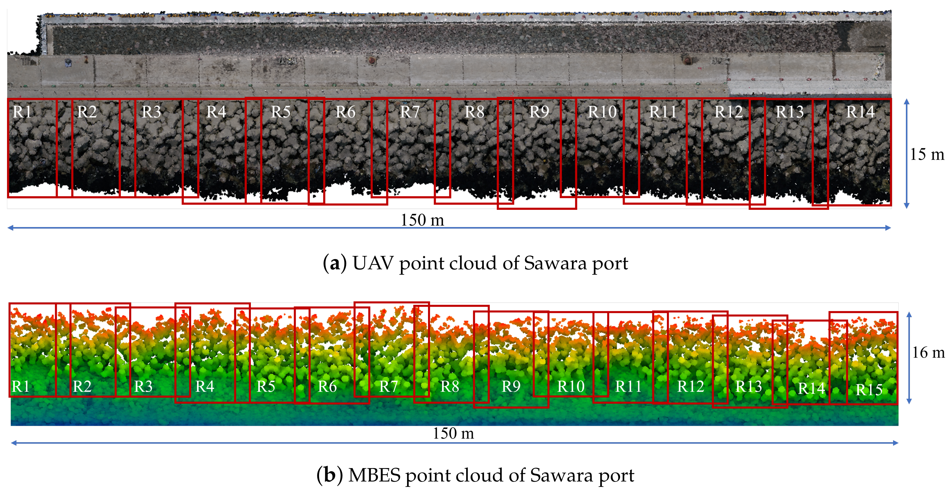
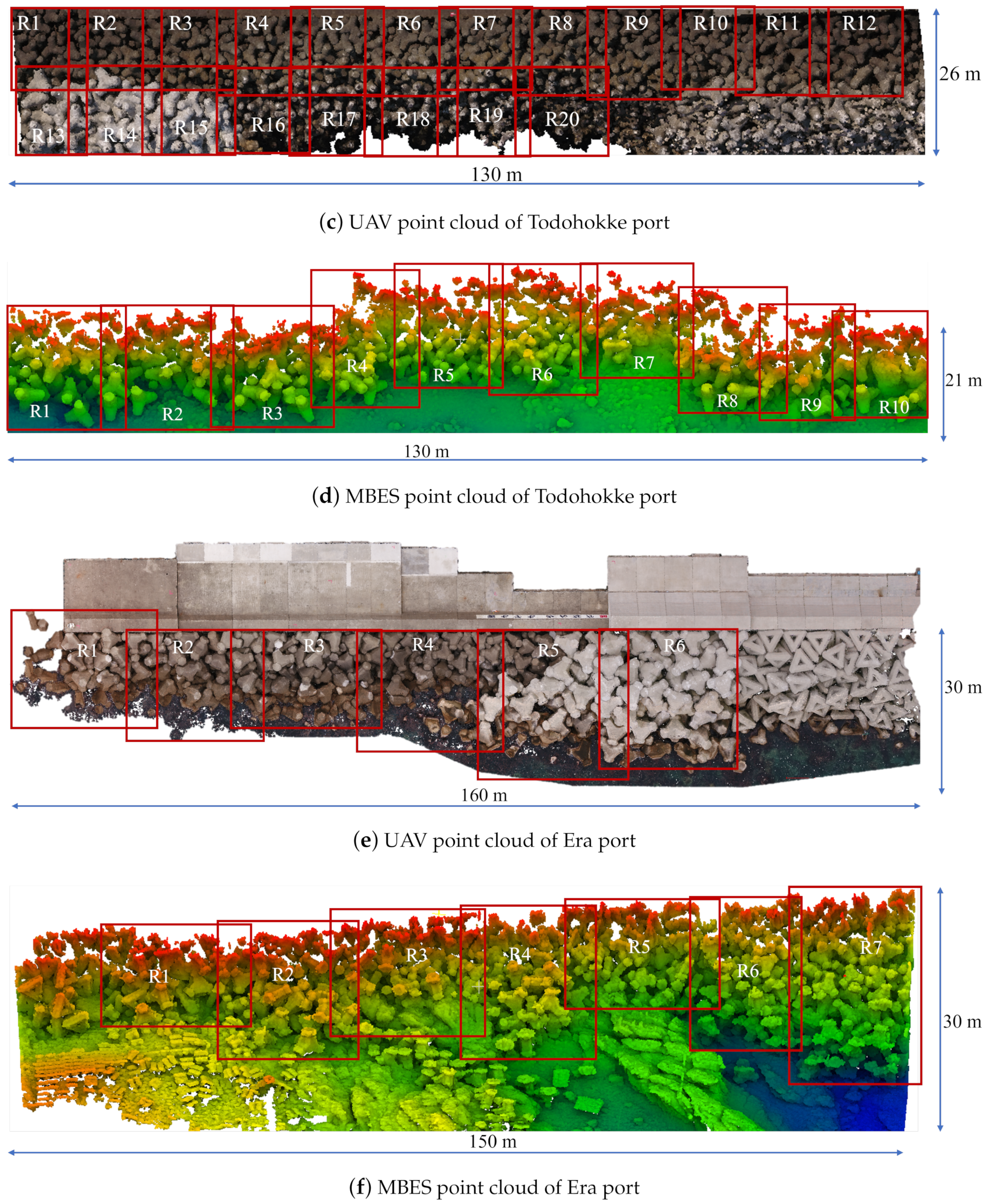
Figure A2.
Additional instance segmentation results on Sawara port (a), Todohokke port (b) and Era port (c). The left column is the point cloud scene measured by UAV. The middle column is the predicted results of instance segmentation, and the last column is the ground truth. Different colors represent different blocks.
References
- Bueno, M.; Díaz-Vilariño, L.; Martínez-Sánchez, J.; González Jorge, H.; Arias, P. 3D reconstruction of cubic armoured rubble mound breakwaters from incomplete lidar data. Int. J. Remote Sens. 2015, 36, 5485–5503. [Google Scholar] [CrossRef]
- González-Jorge, H.; Puente, I.; Roca, D.; Martínez-Sánchez, J.; Conde, B.; Arias, P. UAV Photogrammetry Application to the Monitoring of Rubble Mound Breakwaters. J. Perform. Constr. Facil. 2016, 30, 04014194. [Google Scholar] [CrossRef]
- Stateczny, A.; Błaszczak-Bąk, W.; Sobieraj-Żłobińska, A.; Motyl, W.; Wisniewska, M. Methodology for Processing of 3D Multibeam Sonar Big Data for Comparative Navigation. Remote Sens. 2019, 11, 2245. [Google Scholar] [CrossRef]
- Kulawiak, M.; Lubniewski, Z. Processing of LiDAR and Multibeam Sonar Point Cloud Data for 3D Surface and Object Shape Reconstruction. In Proceedings of the 2016 Baltic Geodetic Congress (BGC Geomatics), Gdansk, Poland, 2 June 2016; pp. 187–190. [Google Scholar] [CrossRef]
- Alevizos, E.; Oikonomou, D.; Argyriou, A.V.; Alexakis, D.D. Fusion of Drone-Based RGB and Multi-Spectral Imagery for Shallow Water Bathymetry Inversion. Remote Sens. 2022, 14, 1127. [Google Scholar] [CrossRef]
- Wang, D.; Xing, S.; He, Y.; Yu, J.; Xu, Q.; Li, P. Evaluation of a New Lightweight UAV-Borne Topo-Bathymetric LiDAR for Shallow Water Bathymetry and Object Detection. Sensors 2022, 22, 1379. [Google Scholar] [CrossRef]
- Dąbrowski, P.S.; Specht, C.; Specht, M.; Burdziakowski, P.; Makar, A.; Lewicka, O. Integration of Multi-Source Geospatial Data from GNSS Receivers, Terrestrial Laser Scanners, and Unmanned Aerial Vehicles. Can. J. Remote Sens. 2021, 47, 621–634. [Google Scholar] [CrossRef]
- Sousa, P.J.; Cachaço, A.; Barros, F.; Tavares, P.J.; Moreira, P.M.; Capitão, R.; Neves, M.G.; Franco, E. Structural monitoring of a breakwater using UAVs and photogrammetry. Procedia Struct. Integr. 2022, 37, 167–172. [Google Scholar] [CrossRef]
- Lemos, R.; Loja, M.A.; Rodrigues, J.; Rodrigues, J.A. Photogrammetric analysis of rubble mound breakwaters scale model tests. AIMS Environ. Sci. 2016, 3, 541–559. [Google Scholar] [CrossRef]
- Puente, I.; Sande, J.; González-Jorge, H.; Peña-González, E.; Maciñeira, E.; Martínez-Sánchez, J.; Arias, P. Novel image analysis approach to the terrestrial LiDAR monitoring of damage in rubble mound breakwaters. Ocean Eng. 2014, 91, 273–280. [Google Scholar] [CrossRef]
- Gonçalves, D.; Gonçalves, G.; Pérez-Alvávez, J.A.; Andriolo, U. On the 3D Reconstruction of Coastal Structures by Unmanned Aerial Systems with Onboard Global Navigation Satellite System and Real-Time Kinematics and Terrestrial Laser Scanning. Remote Sens. 2022, 14, 1485. [Google Scholar] [CrossRef]
- Musumeci, R.E.; Moltisanti, D.; Foti, E.; Battiato, S.; Farinella, G.M. 3-D monitoring of rubble mound breakwater damages. Measurement 2018, 117, 347–364. [Google Scholar] [CrossRef]
- Shen, Y.; Lindenbergh, R.; Wang, J.; Ferreira, V.G. Extracting Individual Bricks from a Laser Scan Point Cloud of an Unorganized Pile of Bricks. Remote Sens. 2018, 10, 1709. [Google Scholar] [CrossRef]
- Xu, Y.; Arai, S.; Liu, D.; Lin, F.; Kosuge, K. FPCC: Fast point cloud clustering-based instance segmentation for industrial bin-picking. Neurocomputing 2022, 494, 255–268. [Google Scholar] [CrossRef]
- Drost, B.; Ulrich, M.; Navab, N.; Ilic, S. Model globally, match locally: Efficient and robust 3D object recognition. In Proceedings of the 2010 IEEE Computer Society Conference on Computer Vision and Pattern Recognition, San Francisco, CA, USA, 13 June 2010; pp. 998–1005. [Google Scholar] [CrossRef]
- Besl, P.J.; McKay, N.D. Method for registration of 3-D shapes. In Sensor Fusion IV: Control Paradigms and Data Structures; Schenker, P.S., Ed.; International Society for Optics and Photonics, SPIE: Boston, MA, USA, 1992; Volume 1611, pp. 586–606. [Google Scholar] [CrossRef]
- Coumans, E.; Bai, Y. PyBullet, a Python Module for Physics Simulation for Games, Robotics and Machine Learning. 2016–2021. Available online: http://pybullet.org (accessed on 9 September 2022).
- Tulsi, K.; Phelp, D. Monitoring and Maintenance of Breakwaters Which Protect Port Entrances. 2009. Available online: http://hdl.handle.net/10204/4139 (accessed on 30 October 2022).
- Campos, Á.; Castillo, C.; Molina-Sanchez, R. Damage in Rubble Mound Breakwaters. Part I: Historical Review of Damage Models. J. Mar. Sci. Eng. 2020, 8, 317. [Google Scholar] [CrossRef]
- Campos, Á.; Molina-Sanchez, R.; Castillo, C. Damage in Rubble Mound Breakwaters. Part II: Review of the Definition, Parameterization, and Measurement of Damage. J. Mar. Sci. Eng. 2020, 8, 306. [Google Scholar] [CrossRef]
- Lemos, R.; Reis, M.T.; Fortes, C.J.; Peña, E.; Sande, J.; Figuero, A.; Alvarellos, A.; Laino, E.; Santos, J.; Kerpen, N.B. Measuring Armour Layer Damage in Rubble-Mound Breakwaters under Oblique Wave Incidence. 2019. Available online: https://henry.baw.de/handle/20.500.11970/106641 (accessed on 30 October 2022).
- Bueno, M.; Díaz-Vilariño, L.; González-Jorge, H.; Martínez-Sánchez, J.; Arias, P. Automatic modelling of rubble mound breakwaters from lidar data. Int. Arch. Photogramm. Remote Sens. Spat. Inf. Sci. 2015, 40, 9. [Google Scholar] [CrossRef]
- Wang, W.; Yu, R.; Huang, Q.; Neumann, U. SGPN: Similarity Group Proposal Network for 3D Point Cloud Instance Segmentation. In Proceedings of the 2018 IEEE/CVF Conference on Computer Vision and Pattern Recognition, Salt Lake, UT, USA, 18 June 2018; pp. 2569–2578. [Google Scholar] [CrossRef]
- Lahoud, J.; Ghanem, B.; Oswald, M.R.; Pollefeys, M. 3D Instance Segmentation via Multi-Task Metric Learning. In Proceedings of the 2019 IEEE/CVF International Conference on Computer Vision (ICCV), Seoul, Korea, 27 October 2019; pp. 9255–9265. [Google Scholar] [CrossRef]
- Pham, Q.; Nguyen, T.; Hua, B.; Roig, G.; Yeung, S. JSIS3D: Joint Semantic-Instance Segmentation of 3D Point Clouds With Multi-Task Pointwise Networks and Multi-Value Conditional Random Fields. In Proceedings of the 2019 IEEE/CVF Conference on Computer Vision and Pattern Recognition (CVPR), Long Beach, CA, USA, 15 June 2019; pp. 8819–8828. [Google Scholar] [CrossRef]
- Wang, X.; Liu, S.; Shen, X.; Shen, C.; Jia, J. Associatively Segmenting Instances and Semantics in Point Clouds. In Proceedings of the 2019 IEEE/CVF Conference on Computer Vision and Pattern Recognition (CVPR), Long Beach, CA, USA, 15 June 2019; pp. 4091–4100. [Google Scholar] [CrossRef]
- Xu, Y.; Arai, S.; Tokuda, F.; Kosuge, K. A Convolutional Neural Network for Point Cloud Instance Segmentation in Cluttered Scene Trained by Synthetic Data Without Color. IEEE Access 2020, 8, 70262–70269. [Google Scholar] [CrossRef]
- Jiang, L.; Zhao, H.; Shi, S.; Liu, S.; Fu, C.W.; Jia, J. PointGroup: Dual-Set Point Grouping for 3D Instance Segmentation. In Proceedings of the 2020 IEEE/CVF Conference on Computer Vision and Pattern Recognition (CVPR), Seattle, WA, USA, 13 June 2020; pp. 4866–4875. [Google Scholar] [CrossRef]
- Chen, S.; Fang, J.; Zhang, Q.; Liu, W.; Wang, X. Hierarchical aggregation for 3d instance segmentation. In Proceedings of the IEEE/CVF International Conference on Computer Vision, Online, 10 March 2021; pp. 15467–15476. [Google Scholar]
- Armeni, I.; Sener, O.; Zamir, A.R.; Jiang, H.; Brilakis, I.; Fischer, M.; Savarese, S. 3D Semantic Parsing of Large-Scale Indoor Spaces. In Proceedings of the 2016 IEEE Conference on Computer Vision and Pattern Recognition (CVPR), Las Vegas, NV, USA, 27 June 2016; pp. 1534–1543. [Google Scholar] [CrossRef]
- Dai, A.; Chang, A.X.; Savva, M.; Halber, M.; Funkhouser, T.; Nießner, M. ScanNet: Richly-Annotated 3D Reconstructions of Indoor Scenes. In Proceedings of the 2017 IEEE Conference on Computer Vision and Pattern Recognition (CVPR), Honolulu, HI, USA, 21 July 2017; pp. 2432–2443. [Google Scholar] [CrossRef]
- Hua, B.; Pham, Q.; Nguyen, D.T.; Tran, M.; Yu, L.; Yeung, S. SceneNN: A Scene Meshes Dataset with aNNotations. In Proceedings of the 2016 Fourth International Conference on 3D Vision (3DV), Stanford, CA, USA, 25 October 2016; pp. 92–101. [Google Scholar] [CrossRef]
- Zhang, F.; Guan, C.; Fang, J.; Bai, S.; Yang, R.; Torr, P.H.; Prisacariu, V. Instance Segmentation of LiDAR Point Clouds. In Proceedings of the 2020 IEEE International Conference on Robotics and Automation (ICRA), Paris, France, 31 May 2020; pp. 9448–9455. [Google Scholar] [CrossRef]
- Walicka, A.; Pfeifer, N. Automatic Segmentation of Individual Grains From a Terrestrial Laser Scanning Point Cloud of a Mountain River Bed. IEEE J. Sel. Top. Appl. Earth Obs. Remote Sens. 2022, 15, 1389–1410. [Google Scholar] [CrossRef]
- Luo, H.; Khoshelham, K.; Chen, C.; He, H. Individual tree extraction from urban mobile laser scanning point clouds using deep pointwise direction embedding. ISPRS J. Photogramm. Remote. Sens. 2021, 175, 326–339. [Google Scholar] [CrossRef]
- Djuricic, A.; Dorninger, P.; Nothegger, C.; Harzhauser, M.; Székely, B.; Rasztovits, S.; Mandic, O.; Molnár, G.; Pfeifer, N. High-resolution 3D surface modeling of a fossil oyster reef. Geosphere 2016, 12, 1457–1477. [Google Scholar] [CrossRef][Green Version]
- Salti, S.; Tombari, F.; Di Stefano, L. SHOT: Unique signatures of histograms for surface and texture description. Comput. Vis. Image Underst. 2014, 125, 251–264. [Google Scholar] [CrossRef]
- Rusu, R.B.; Blodow, N.; Marton, Z.C.; Beetz, M. Aligning point cloud views using persistent feature histograms. In Proceedings of the 2008 IEEE/RSJ International Conference on Intelligent Robots and Systems, Nice, France, 22 September 2008; pp. 3384–3391. [Google Scholar] [CrossRef]
- Abbeloos, W.; Goedemé, T. Point Pair Feature Based Object Detection for Random Bin Picking. In Proceedings of the 2016 13th Conference on Computer and Robot Vision (CRV), Victoria, BC, Canada, 1 June 2016; pp. 432–439. [Google Scholar] [CrossRef]
- Hinterstoisser, S.; Lepetit, V.; Rajkumar, N.; Konolige, K. Going Further with Point Pair Features. In Computer Vision—ECCV 2016; Leibe, B., Matas, J., Sebe, N., Welling, M., Eds.; Springer International Publishing: Cham, Switzerland, 2016; pp. 834–848. [Google Scholar]
- Liu, D.; Arai, S.; Miao, J.; Kinugawa, J.; Wang, Z.; Kosuge, K. Point Pair Feature-Based Pose Estimation with Multiple Edge Appearance Models (PPF-MEAM) for Robotic Bin Picking. Sensors 2018, 18, 2719. [Google Scholar] [CrossRef] [PubMed]
- Birdal, T.; Ilic, S. Point Pair Features Based Object Detection and Pose Estimation Revisited. In Proceedings of the 2015 International Conference on 3D Vision, Lyon, France, 19 October 2015; pp. 527–535. [Google Scholar] [CrossRef]
- Xiang, Y.; Schmidt, T.; Narayanan, V.; Fox, D. PoseCNN: A Convolutional Neural Network for 6D Object Pose Estimation in Cluttered Scenes. 2018. Available online: https://github.com/yuxng/PoseCNN (accessed on 30 October 2022).
- Wang, C.; Xu, D.; Zhu, Y.; Martín-Martín, R.; Lu, C.; Fei-Fei, L.; Savarese, S. DenseFusion: 6D Object Pose Estimation by Iterative Dense Fusion. In Proceedings of the 2019 IEEE/CVF Conference on Computer Vision and Pattern Recognition (CVPR), Long Beach, CA, USA, 15 June 2019; pp. 3338–3347. [Google Scholar] [CrossRef]
- Dong, Z.; Liu, S.; Zhou, T.; Cheng, H.; Zeng, L.; Yu, X.; Liu, H. PPR-Net:Point-wise Pose Regression Network for Instance Segmentation and 6D Pose Estimation in Bin-picking Scenarios. In Proceedings of the 2019 IEEE/RSJ International Conference on Intelligent Robots and Systems (IROS), Macau, China, 3 November 2019; pp. 1773–1780. [Google Scholar] [CrossRef]
- Zeng, L.; Lv, W.J.; Dong, Z.K.; Liu, Y.J. PPR-Net++: Accurate 6-D Pose Estimation in Stacked Scenarios. IEEE Trans. Autom. Sci. Eng. 2021, 19, 3139–3151. [Google Scholar] [CrossRef]
- Deng, X.; Mousavian, A.; Xiang, Y.; Xia, F.; Bretl, T.; Fox, D. PoseRBPF: A Rao–Blackwellized Particle Filter for 6-D Object Pose Tracking. IEEE Trans. Robot. 2021, 37, 1328–1342. [Google Scholar] [CrossRef]
- Deng, X.; Xiang, Y.; Mousavian, A.; Eppner, C.; Bretl, T.; Fox, D. Self-supervised 6D Object Pose Estimation for Robot Manipulation. In Proceedings of the 2020 IEEE International Conference on Robotics and Automation (ICRA), Paris, France, 31 May 2020; pp. 3665–3671. [Google Scholar] [CrossRef]
- Yin, Y.; Cai, Y.; Wang, H.; Chen, B. FisherMatch: Semi-Supervised Rotation Regression via Entropy-based Filtering. In Proceedings of the 2022 IEEE/CVF Conference on Computer Vision and Pattern Recognition (CVPR), New Orleans, LA, USA, 18–24 June 2022. [Google Scholar] [CrossRef]
- Wang, Y.; Sun, Y.; Liu, Z.; Sarma, S.E.; Bronstein, M.M.; Solomon, J.M. Dynamic Graph CNN for Learning on Point Clouds. ACM Trans. Graph. 2019, 38, 1–12. [Google Scholar] [CrossRef]
- Liu, D.; Arai, S.; Xu, Y.; Tokuda, F.; Kosuge, K. 6D Pose Estimation of Occlusion-Free Objects for Robotic Bin-Picking using PPF-MEAM with 2D Images (Occlusion-Free PPF-MEAM). IEEE Access 2021, 9, 50857–50871. [Google Scholar] [CrossRef]
- Li, G.; Mueller, M.; Qian, G.; Delgadillo Perez, I.C.; Abualshour, A.; Thabet, A.K.; Ghanem, B. DeepGCNs: Making GCNs Go as Deep as CNNs. IEEE Trans. Pattern Anal. Mach. Intell. 2021. [Google Scholar] [CrossRef]
- Luo, W.; Li, Y.; Urtasun, R.; Zemel, R. Understanding the Effective Receptive Field in Deep Convolutional Neural Networks. In Advances in Neural Information Processing Systems; Lee, D., Sugiyama, M., Luxburg, U., Guyon, I., Garnett, R., Eds.; Curran Associates, Inc.: Barcelona, Spain, 2016; Volume 29. [Google Scholar]
- Engelmann, F.; Kontogianni, T.; Leibe, B. Dilated Point Convolutions: On the Receptive Field Size of Point Convolutions on 3D Point Clouds. In Proceedings of the 2020 IEEE International Conference on Robotics and Automation (ICRA), Paris, France, 31 May 2020; pp. 9463–9469. [Google Scholar] [CrossRef]
- Qi, C.R.; Yi, L.; Su, H.; Guibas, L.J. PointNet++: Deep Hierarchical Feature Learning on Point Sets in a Metric Space. In Proceedings of the 31st International Conference on Neural Information Processing Systems (NIPS’17), Long Beach, CA, USA, 4 December 2017; Curran Associates Inc.: Red Hook, NY, USA, 2017; pp. 5105–5114. [Google Scholar]
- Li, R.; Wang, S.; Zhu, F.; Huang, J. Adaptive Graph Convolutional Neural Networks. In Proceedings of the AAAI Conference on Artificial Intelligence, New Orleans, LA, USA, 2 February 2018; Volume 32. [Google Scholar]
- Hu, Q.; Yang, B.; Xie, L.; Rosa, S.; Guo, Y.; Wang, Z.; Trigoni, N.; Markham, A. RandLA-Net: Efficient Semantic Segmentation of Large-Scale Point Clouds. In Proceedings of the 2020 IEEE/CVF Conference on Computer Vision and Pattern Recognition (CVPR), Seattle, WA, USA, 13 June 2020; pp. 11105–11114. [Google Scholar] [CrossRef]
- Yang, B.; Wang, S.; Markham, A.; Trigoni, N. Robust attentional aggregation of deep feature sets for multi-view 3D reconstruction. Int. J. Comput. Vis. 2020, 128, 53–73. [Google Scholar] [CrossRef]
- Tobin, J.; Fong, R.; Ray, A.; Schneider, J.; Zaremba, W.; Abbeel, P. Domain randomization for transferring deep neural networks from simulation to the real world. In Proceedings of the 2017 IEEE/RSJ International Conference on Intelligent Robots and Systems (IROS), Vancouver, BC, Canada, 24 September 2017; pp. 23–30. [Google Scholar] [CrossRef]
- Planche, B.; Wu, Z.; Ma, K.; Sun, S.; Kluckner, S.; Lehmann, O.; Chen, T.; Hutter, A.; Zakharov, S.; Kosch, H.; et al. DepthSynth: Real-Time Realistic Synthetic Data Generation from CAD Models for 2.5D Recognition. In Proceedings of the 2017 International Conference on 3D Vision (3DV), Qingdao, China, 10 October 2017; pp. 1–10. [Google Scholar] [CrossRef]
- Tremblay, J.; Prakash, A.; Acuna, D.; Brophy, M.; Jampani, V.; Anil, C.; To, T.; Cameracci, E.; Boochoon, S.; Birchfield, S. Training Deep Networks with Synthetic Data: Bridging the Reality Gap by Domain Randomization. In Proceedings of the 2018 IEEE/CVF Conference on Computer Vision and Pattern Recognition Workshops (CVPRW), Salt Lake, UT, USA, 18 June 2018; pp. 1082–10828. [Google Scholar] [CrossRef]
- Katz, S.; Tal, A.; Basri, R. Direct Visibility of Point Sets. In ACM SIGGRAPH 2007 Papers; SIGGRAPH ’07; Association for Computing Machinery: New York, NY, USA, 2007; p. 24. [Google Scholar] [CrossRef]
- Brégier, R.; Devernay, F.; Leyrit, L.; Crowley, J.L. Defining the pose of any 3d rigid object and an associated distance. Int. J. Comput. Vis. 2018, 126, 571–596. [Google Scholar] [CrossRef]
- Johnson, A.; Hebert, M. Using spin images for efficient object recognition in cluttered 3D scenes. IEEE Trans. Pattern Anal. Mach. Intell. 1999, 21, 433–449. [Google Scholar] [CrossRef]
Publisher’s Note: MDPI stays neutral with regard to jurisdictional claims in published maps and institutional affiliations. |
© 2022 by the authors. Licensee MDPI, Basel, Switzerland. This article is an open access article distributed under the terms and conditions of the Creative Commons Attribution (CC BY) license (https://creativecommons.org/licenses/by/4.0/).


