
Accuracy Assessment of Photochemical Reflectance Index (PRI) and Chlorophyll Carotenoid Index (CCI) Derived from GCOM-C/SGLI with In Situ Data

 ,
,  , , , and
Abstract
1. Introduction
2. Materials and Methods
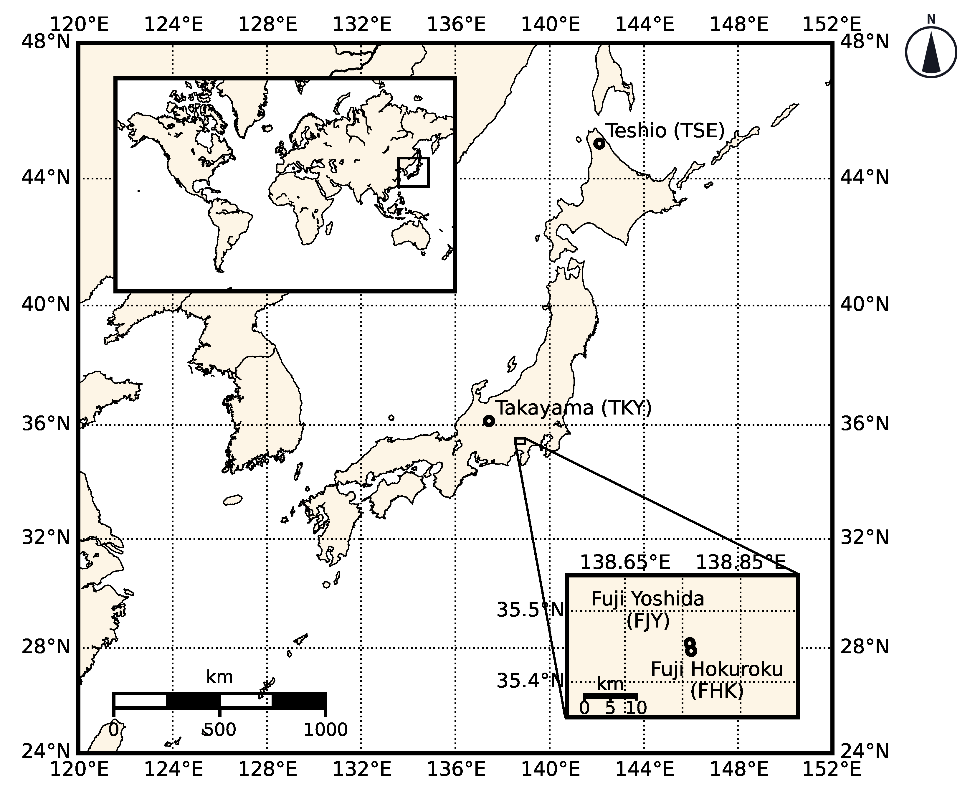
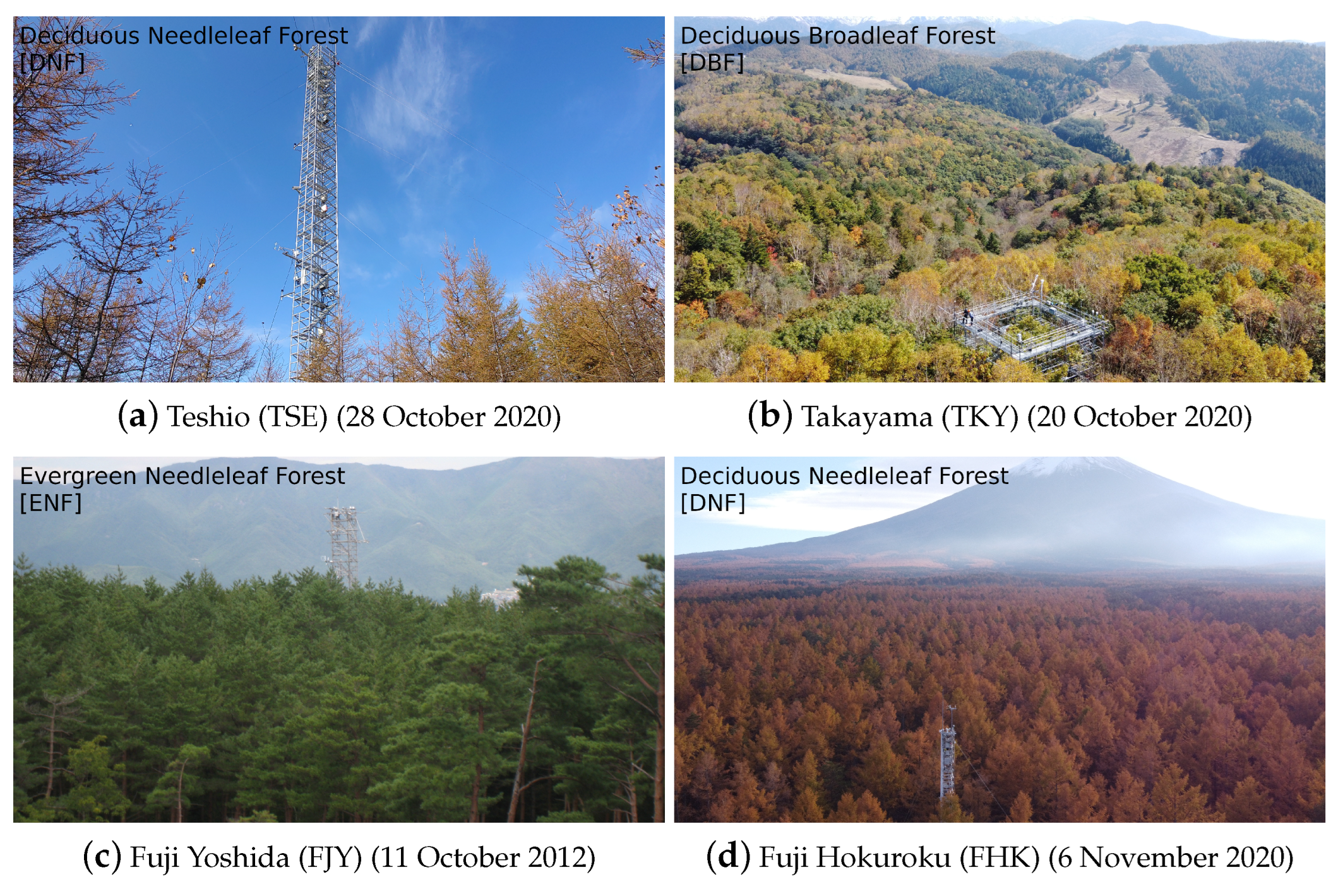
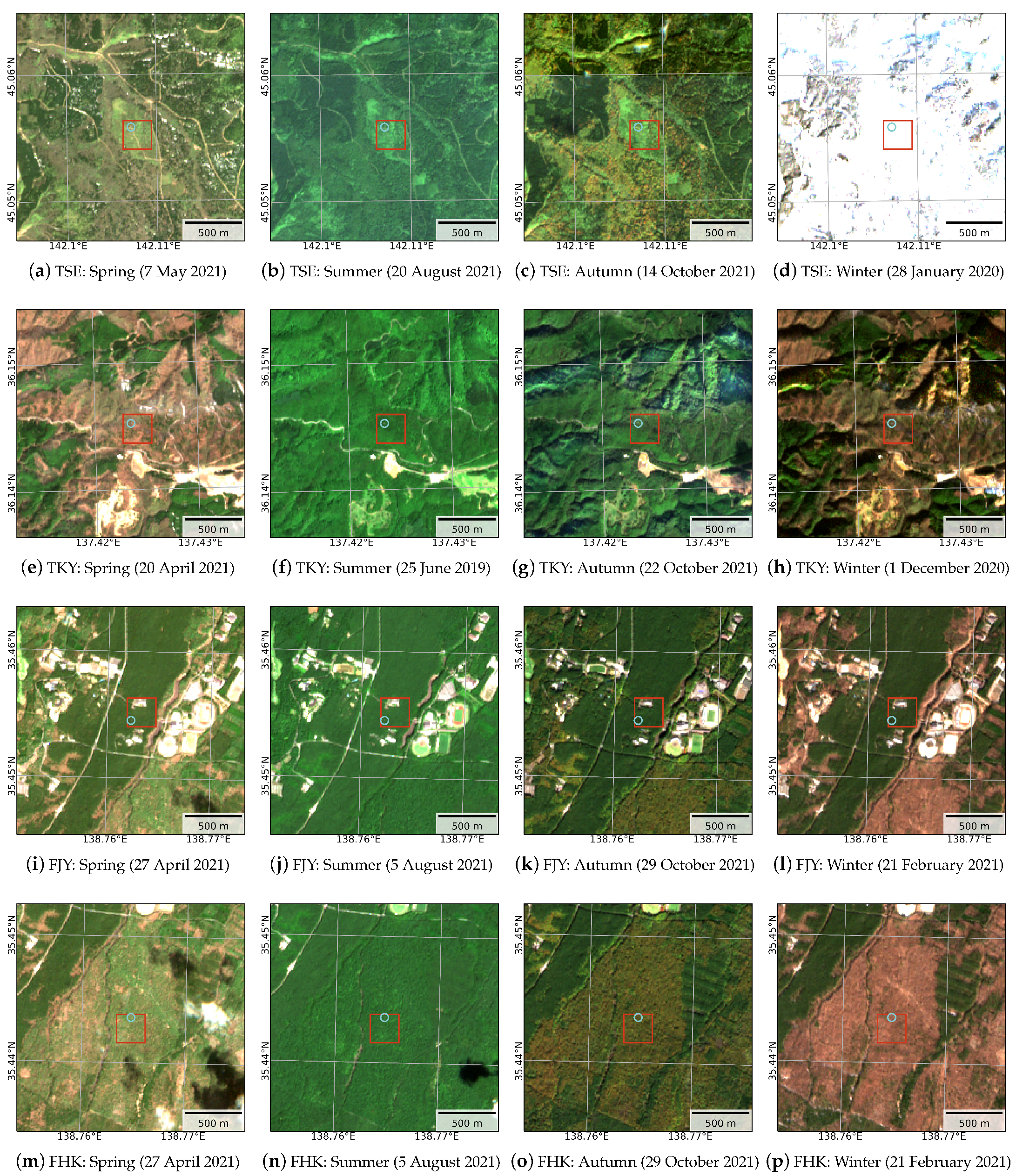
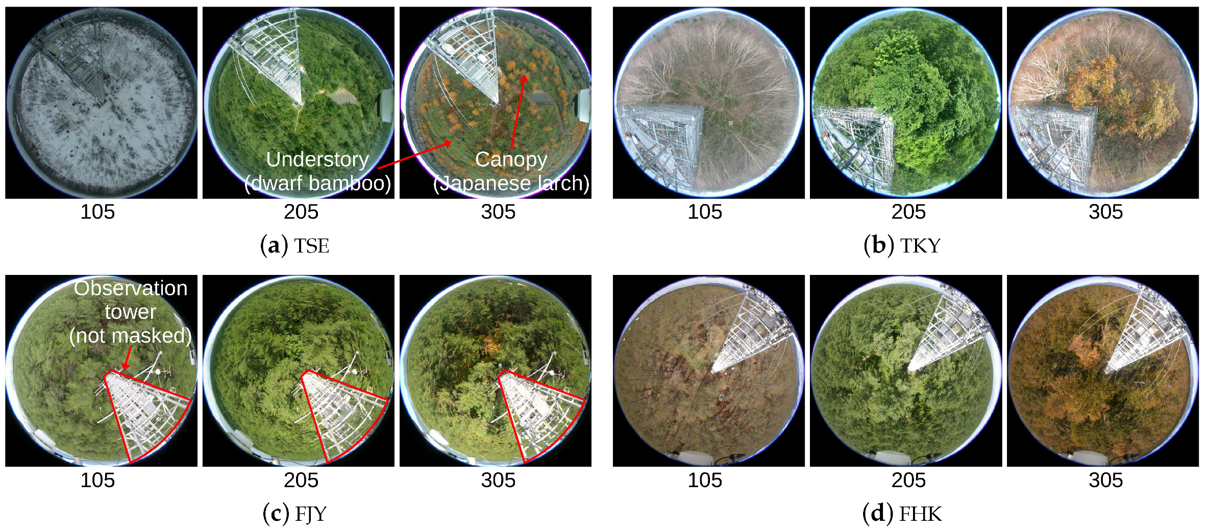
2.1. Study Sites
2.2. In Situ Data
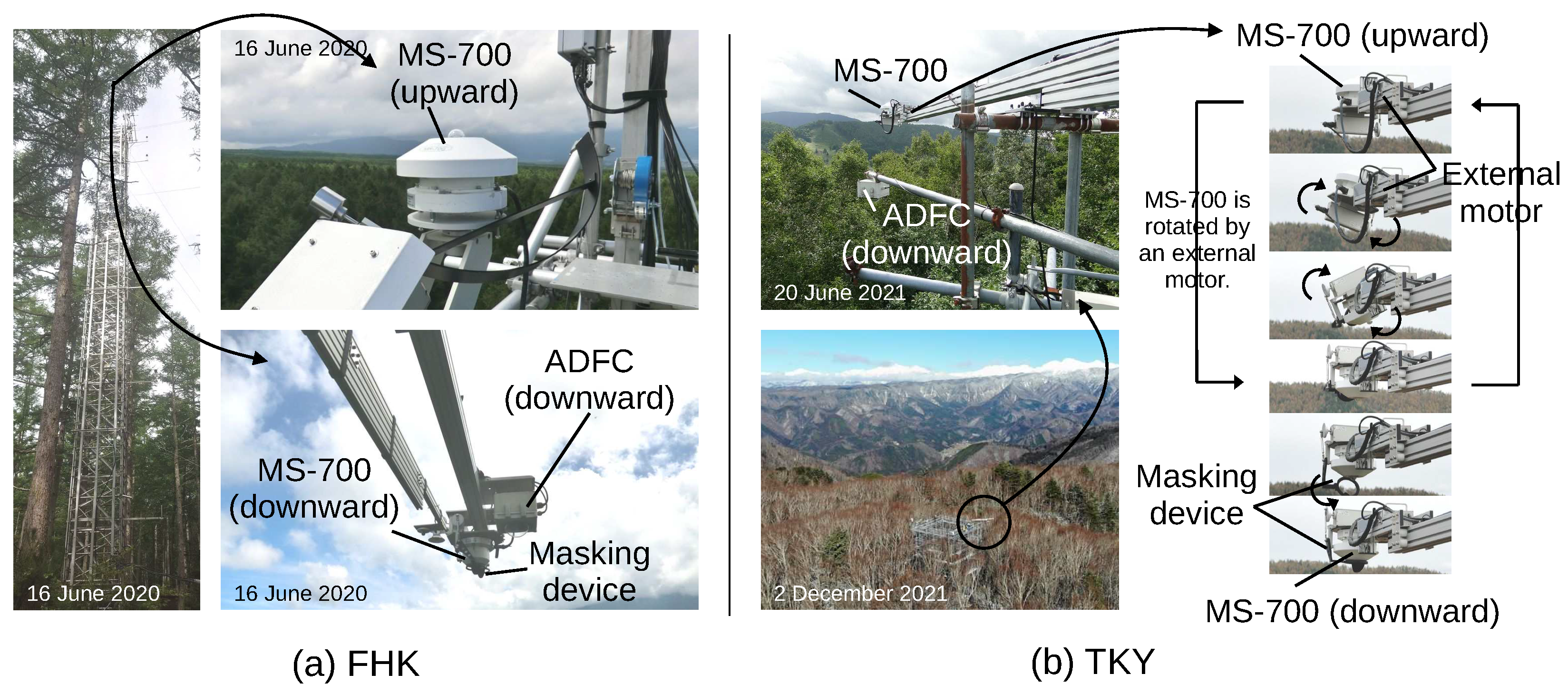
2.2.1. In Situ Data Collection
2.2.2. In Situ Data Processing
2.3. Satellite Data
2.3.1. Satellite Data Collection
2.3.2. Satellite Data Processing
2.4. Comparison and Statistical Analysis
3. Results
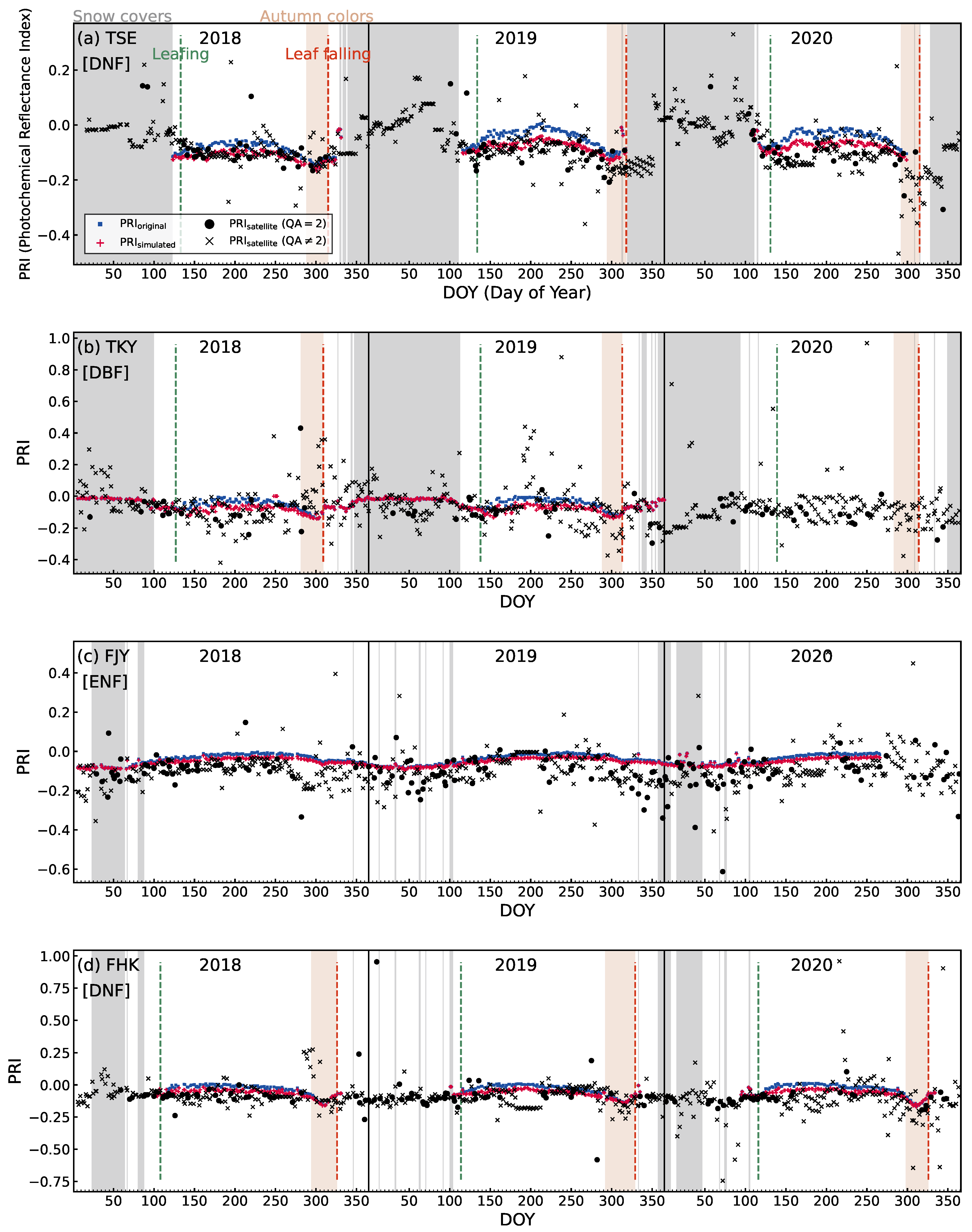
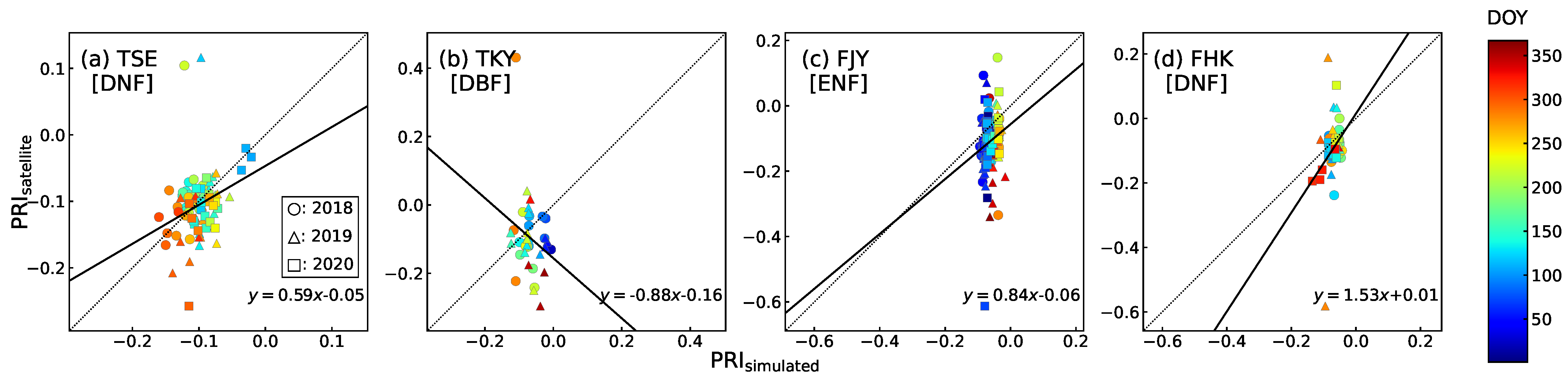
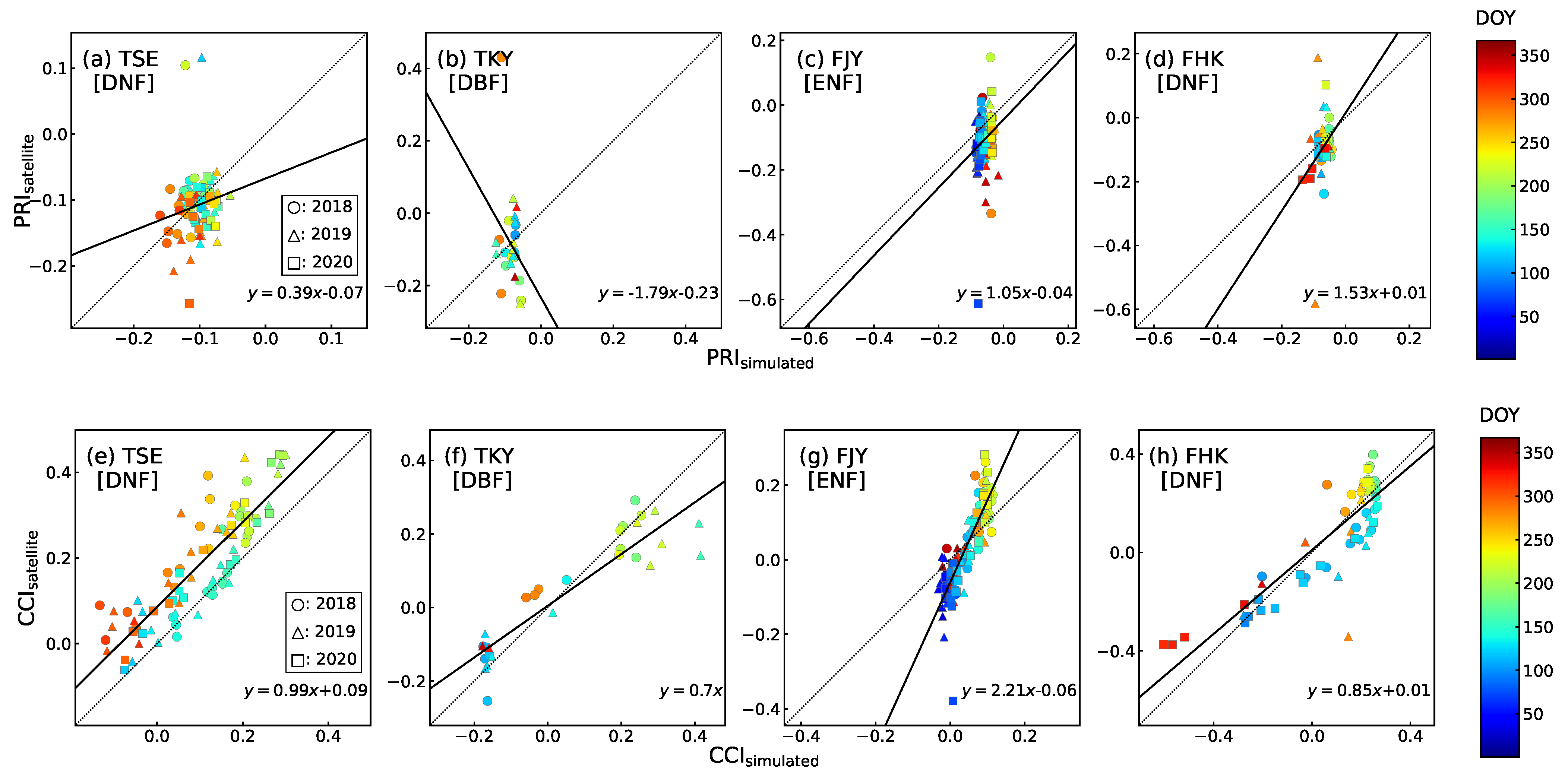
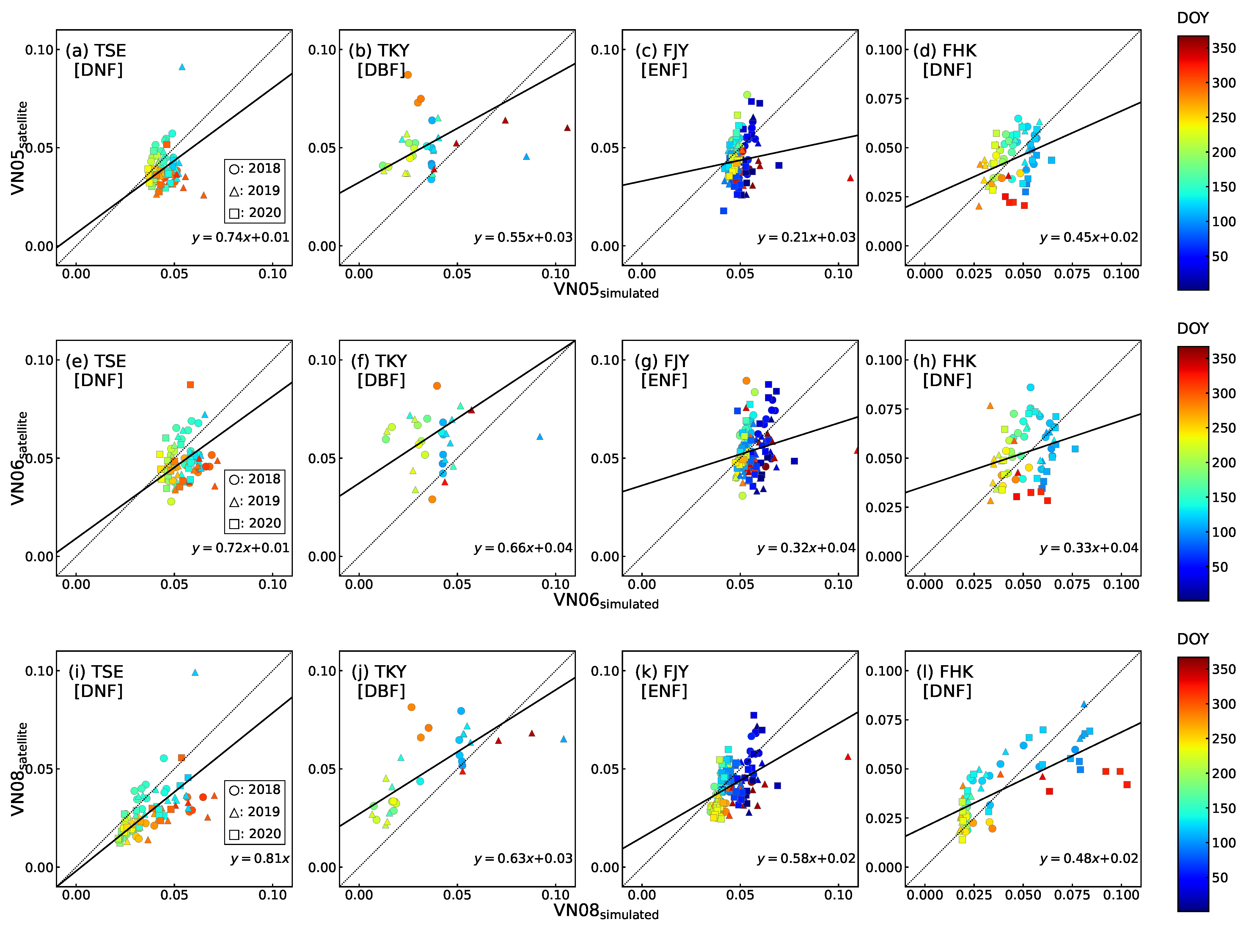
3.1. Accuracy Assessment of PRI
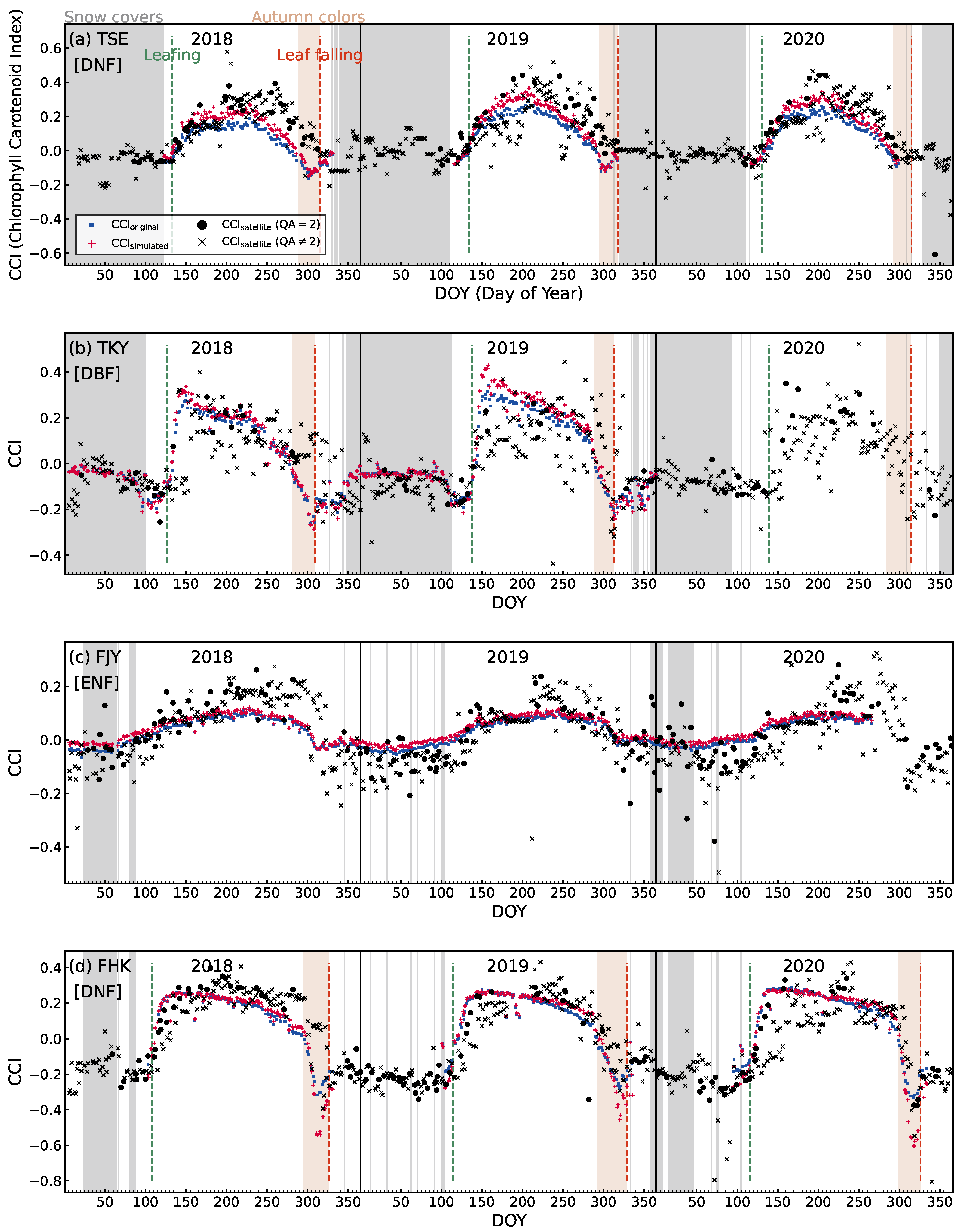
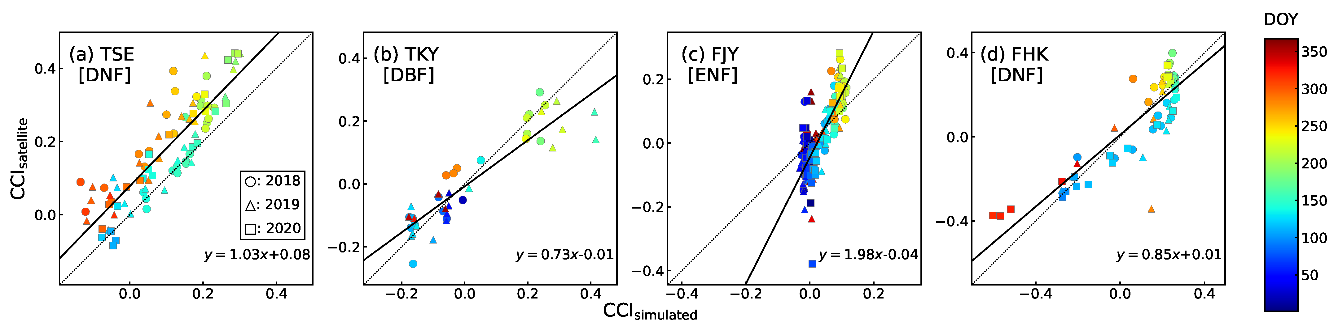
3.2. Accuracy Assessment of CCI
4. Discussion
4.1. Common Outliers for and
4.2. Unique Outliers for
4.2.1. Striping Outliers
4.2.2. Cluster Outliers
4.3. Demonstrations of Removing the Outliers
4.4. Small Noise and Index Design
4.5. Footprint Effects for Accuracy Assessment of
5. Conclusions
Author Contributions
Funding
Data Availability Statement
Acknowledgments
Conflicts of Interest
Appendix A

| Site ID and Period | Direction of MS-700 | The Nearest Neighbor Band’s Peak to 531 nm | The Second Nearest Neighbor Band’s Peak to 531 nm | The Nearest Neighbor Band’s Peak to 570 nm | The Second Nearest Neighbor Band’s Peak to 570 nm | The Nearest Neighbor Band’s Peak to 645 nm | The Second Nearest Neighbor Band’s Peak to 645 nm |
|---|---|---|---|---|---|---|---|
| TSE 2018-01-01 – 2020-12-31 | upward | nm | nm | nm | nm | nm | nm |
| downward | nm | nm | nm | nm | nm | nm | |
| TKY 2018-01-01 – 2019-05-07 | upward | nm | nm | nm | nm | nm | nm |
| downward | nm | nm | nm | nm | nm | nm | |
| TKY 2019-05-08 – 2020-12-31 | upward | nm | nm | nm | nm | nm | nm |
| downward | nm | nm | nm | nm | nm | nm | |
| FJY 2018-01-01 – 2020-12-31 | upward | nm | nm | nm | nm | nm | nm |
| downward | nm | nm | nm | nm | nm | nm | |
| FHK 2018-01-01 – 2018-12-31 | upward | nm | nm | nm | nm | nm | nm |
| downward | nm | nm | nm | nm | nm | nm | |
| FHK 2019-01-01 – 2020-12-31 | upward | nm | nm | nm | nm | nm | nm |
| downward | nm | nm | nm | nm | nm | nm |

| Site ID | n | r | RMSE | MAE | |
|---|---|---|---|---|---|
| VN05 | TSE | 84 | () | 0.016 | 0.010 |
| TKY | 40 | () | 0.032 | 0.026 | |
| FJY | 146 | () | 4.948 | 4.908 | |
| FHK | 65 | () | 0.012 | 0.010 | |
| VN05 | TSE | 84 | () | 0.017 | 0.012 |
| TKY | 40 | () | 0.037 | 0.030 | |
| FJY | 146 | () | 5.594 | 5.550 | |
| FHK | 65 | () | 0.015 | 0.013 | |
| VN05 | TSE | 84 | () | 0.019 | 0.014 |
| TKY | 40 | () | 0.031 | 0.024 | |
| FJY | 146 | () | 4.697 | 4.621 | |
| FHK | 65 | () | 0.017 | 0.013 |
References
- Gamon, J.A.; Field, C.B.; Bilger, W.; Björkman, O.; Fredeen, A.L.; Peñuelas, J. Remote sensing of the xanthophyll cycle and chlorophyll fluorescence in sunflower leaves and canopies. Oecologia 1990, 85, 1–7. [Google Scholar] [CrossRef] [PubMed]
- Gamon, J.A.; Peñuelas, J.; Field, C.B. A narrow-waveband spectral index that tracks diurnal changes in photosynthetic efficiency. Remote Sens. Environ. 1992, 41, 35–44. [Google Scholar] [CrossRef]
- Gamon, J.A.; Serrano, L.; Surfus, J.S. The photochemical reflectance index: An optical indicator of photosynthetic radiation use efficiency across species, functional types, and nutrient levels. Oecologia 1997, 112, 492–501. [Google Scholar] [CrossRef] [PubMed]
- Thenot, F.; Méthy, M.; Winkel, T. The Photochemical Reflectance Index (PRI) as a water-stress index. Int. J. Remote Sens. 2002, 23, 5135–5139. [Google Scholar] [CrossRef]
- Suárez, L.; Zarco-Tejada, P.J.; Sepulcre-Cantó, G.; Pérez-Priego, O.; Miller, J.R.; Jiménez-Muñoz, J.C.; Sobrino, J. Assessing canopy PRI for water stress detection with diurnal airborne imagery. Remote Sens. Environ. 2008, 112, 560–575. [Google Scholar] [CrossRef]
- Porcar-Castell, A.; Garcia-Plazaola, J.I.; Nichol, C.J.; Kolari, P.; Olascoaga, B.; Kuusinen, N.; Fernández-Marín, B.; Pulkkinen, M.; Juurola, E.; Nikinmaa, E. Physiology of the seasonal relationship between the photochemical reflectance index and photosynthetic light use efficiency. Oecologia 2012, 170, 313–323. [Google Scholar] [CrossRef] [PubMed]
- Hmimina, G.; Dufrêne, E.; Soudani, K. Relationship between photochemical reflectance index and leaf ecophysiological and biochemical parameters under two different water statuses: Towards a rapid and efficient correction method using real-time measurements. Plant Cell Environ. 2014, 37, 473–487. [Google Scholar] [CrossRef]
- Springer, K.R.; Wang, R.; Gamon, J.A. Parallel Seasonal Patterns of Photosynthesis, Fluorescence, and Reflectance Indices in Boreal Trees. Remote Sens. 2017, 9, 691. [Google Scholar] [CrossRef]
- Xu, S.; Liu, Z.; Zhao, L.; Zhao, H.; Ren, S. Diurnal Response of Sun-Induced Fluorescence and PRI to Water Stress in Maize Using a Near-Surface Remote Sensing Platform. Remote Sens. 2018, 10, 1510. [Google Scholar] [CrossRef]
- Eitel, J.U.H.; Maguire, A.J.; Boelman, N.; Vierling, L.A.; Griffin, K.L.; Jensen, J.; Magney, T.S.; Mahoney, P.J.; Meddens, A.J.H.; Silva, C.; et al. Proximal remote sensing of tree physiology at northern treeline: Do late-season changes in the photochemical reflectance index (PRI) respond to climate or photoperiod? Remote Sens. Environ. 2019, 221, 340–350. [Google Scholar] [CrossRef]
- Yang, J.C.; Magney, T.S.; Yan, D.; Knowles, J.F.; Smith, W.K.; Scott, R.L.; Barron-Gafford, G.A. The photochemical reflectance index (PRI) captures the ecohydrologic sensitivity of a semiarid mixed conifer forest. J. Geophys. Res. Biogeosci. 2020, 125, e2019JG005624. [Google Scholar] [CrossRef]
- Pierrat, Z.; Nehemy, M.F.; Roy, A.; Magney, T.; Parazoo, N.C.; Laroque, C.; Pappas, C.; Sonnentag, O.; Grossmann, K.; Bowling, D.R.; et al. Tower-based remote sensing reveals mechanisms behind a two-phased spring transition in a mixed-species boreal forest. J. Geophys. Res. Biogeosci. 2021, 126, e2020JG006191. [Google Scholar] [CrossRef]
- Kohzuma, K.; Tamaki, M.; Hikosaka, K. Corrected photochemical reflectance index (PRI) is an effective tool for detecting environmental stresses in agricultural crops under light conditions. J. Plant Res. 2021, 134, 683–694. [Google Scholar] [CrossRef]
- Tsujimoto, K.; Hikosaka, K. Estimating leaf photosynthesis of C3 plants grown under different environments from pigment index, photochemical reflectance index, and chlorophyll fluorescence. Photosynth. Res. 2021, 148, 33–46. [Google Scholar] [CrossRef] [PubMed]
- Filella, I.; Porcar-Castell, A.; Munné-Bosch, S.; Bäck, J.; Garbulsky, M.F.; Peñuelas, J. PRI assessment of long-term changes in carotenoids/chlorophyll ratio and short-term changes in de-epoxidation state of the xanthophyll cycle. Int. J. Remote Sens. 2009, 30, 4443–4455. [Google Scholar] [CrossRef]
- Gamon, J.A.; Kovalchuck, O.; Wong, C.Y.S.; Harris, A.; Garrity, S.R. Monitoring seasonal and diurnal changes in photosynthetic pigments with automated PRI and NDVI sensors. Biogeosciences 2015, 12, 4149–4159. [Google Scholar] [CrossRef]
- Gitelson, A.A.; Gamon, J.A.; Solovchenko, A. Multiple drivers of seasonal change in PRI: Implications for photosynthesis 1. Leaf level. Remote Sens. Environ. 2017, 191, 110–116. [Google Scholar] [CrossRef]
- Gitelson, A.A.; Gamon, J.A.; Solovchenko, A. Multiple drivers of seasonal change in PRI: Implications for photosynthesis 2. Stand level. Remote Sens. Environ. 2017, 190, 198–206. [Google Scholar] [CrossRef]
- Monteith, J.L. Solar Radiation and Productivity in Tropical Ecosystems. J. Appl. Ecol. 1972, 9, 747–766. [Google Scholar] [CrossRef]
- Monteith, J.L.; Moss, C.J.; Cooke, G.W.; Pirie, N.W.; Bell, G.D.H. Climate and the efficiency of crop production in Britain. Philos. Trans. R. Soc. Lond. B Biol. Sci. 1977, 281, 277–294. [Google Scholar] [CrossRef]
- Penuelas, J.; Filella, I.; Gamon, J.A. Assessment of photosynthetic radiation-use efficiency with spectral reflectance. New Phytol. 1995, 131, 291–296. [Google Scholar] [CrossRef]
- Peñuelas, J.; Llusia, J.; Pinol, J.; Filella, I. Photochemical reflectance index and leaf photosynthetic radiation-use-efficiency assessment in Mediterranean trees. Int. J. Remote Sens. 1997, 18, 2863–2868. [Google Scholar] [CrossRef]
- Winkel, T.; Méthy, M.; Thénot, F. Radiation use efficiency, chlorophyll fluorescence, and reflectance indices associated with ontogenic changes in water-limited Chenopodium quinoa leaves. Photosynthetica 2002, 40, 227–232. [Google Scholar] [CrossRef]
- Nakaji, T.; Oguma, H.; Fujinuma, Y. Seasonal changes in the relationship between photochemical reflectance index and photosynthetic light use efficiency of Japanese larch needles. Int. J. Remote Sens. 2006, 27, 493–509. [Google Scholar] [CrossRef]
- Nichol, C.J.; Huemmrich, K.F.; Andrew Black, T.; Jarvis, P.G.; Walthall, C.L.; Grace, J.; Hall, F.G. Remote sensing of photosynthetic-light-use efficiency of boreal forest. Agric. For. Meteorol. 2000, 101, 131–142. [Google Scholar] [CrossRef]
- Nichol, C.J.; Lloyd, J.; Shibistova, O.; Arneth, A.; Röser, C.; Knohl, A.; Matsubara, S.; Grace, J. Remote sensing of photosynthetic-light-use efficiency of a Siberian boreal forest. Tellus B Chem. Phys. Meteorol. 2002, 54, 677–687. [Google Scholar] [CrossRef]
- Nakaji, T.; Ide, R.; Oguma, H.; Saigusa, N.; Fujinuma, Y. Utility of spectral vegetation index for estimation of gross CO2 flux under varied sky conditions. Remote Sens. Environ. 2007, 109, 274–284. [Google Scholar] [CrossRef]
- Hall, F.G.; Hilker, T.; Coops, N.C.; Lyapustin, A.; Huemmrich, K.F.; Middleton, E.; Margolis, H.; Drolet, G.; Black, T.A. Multi-angle remote sensing of forest light use efficiency by observing PRI variation with canopy shadow fraction. Remote Sens. Environ. 2008, 112, 3201–3211. [Google Scholar] [CrossRef]
- Garbulsky, M.F.; Peñuelas, J.; Gamon, J.; Inoue, Y.; Filella, I. The photochemical reflectance index (PRI) and the remote sensing of leaf, canopy and ecosystem radiation use efficiencies: A review and meta-analysis. Remote Sens. Environ. 2011, 115, 281–297. [Google Scholar] [CrossRef]
- Zhang, C.; Filella, I.; Garbulsky, M.; Peñuelas, J. Affecting Factors and Recent Improvements of the Photochemical Reflectance Index (PRI) for Remotely Sensing Foliar, Canopy and Ecosystemic Radiation-Use Efficiencies. Remote Sens. 2016, 8, 677. [Google Scholar] [CrossRef]
- Huang, W.; Lamb, D.W.; Niu, Z.; Zhang, Y.; Liu, L.; Wang, J. Identification of yellow rust in wheat using in-situ spectral reflectance measurements and airborne hyperspectral imaging. Precis. Agric. 2007, 8, 187–197. [Google Scholar] [CrossRef]
- Stagakis, S.; Markos, N.; Sykioti, O.; Kyparissis, A. Monitoring canopy biophysical and biochemical parameters in ecosystem scale using satellite hyperspectral imagery: An application on a Phlomis fruticosa Mediterranean ecosystem using multiangular CHRIS/PROBA observations. Remote Sens. Environ. 2010, 114, 977–994. [Google Scholar] [CrossRef]
- Rossini, M.; Fava, F.; Cogliati, S.; Meroni, M.; Marchesi, A.; Panigada, C.; Giardino, C.; Busetto, L.; Migliavacca, M.; Amaducci, S.; et al. Assessing canopy PRI from airborne imagery to map water stress in maize. ISPRS J. Photogramm. Remote Sens. 2013, 86, 168–177. [Google Scholar] [CrossRef]
- Stagakis, S.; Markos, N.; Sykioti, O.; Kyparissis, A. Tracking seasonal changes of leaf and canopy light use efficiency in a Phlomis fruticosa Mediterranean ecosystem using field measurements and multi-angular satellite hyperspectral imagery. ISPRS J. Photogramm. Remote Sens. 2014, 97, 138–151. [Google Scholar] [CrossRef]
- Gamon, J.A.; Fred Huemmrich, K.; Wong, C.Y.S.; Ensminger, I.; Garrity, S.; Hollinger, D.Y.; Noormets, A.; Peñuelas, J. A remotely sensed pigment index reveals photosynthetic phenology in evergreen conifers. Proc. Natl. Acad. Sci. USA 2016, 113, 13087–13092. [Google Scholar] [CrossRef] [PubMed]
- Drolet, G.G.; Huemmrich, K.F.; Hall, F.G.; Middleton, E.M.; Black, T.A.; Barr, A.G.; Margolis, H.A. A MODIS-derived photochemical reflectance index to detect inter-annual variations in the photosynthetic light-use efficiency of a boreal deciduous forest. Remote Sens. Environ. 2005, 98, 212–224. [Google Scholar] [CrossRef]
- Middleton, E.M.; Huemmrich, K.F.; Landis, D.R.; Black, T.A.; Barr, A.G.; McCaughey, J.H. Photosynthetic efficiency of northern forest ecosystems using a MODIS-derived Photochemical Reflectance Index (PRI). Remote Sens. Environ. 2016, 187, 345–366. [Google Scholar] [CrossRef]
- Kim, J.; Ryu, Y.; Dechant, B.; Lee, H.; Kim, H.S.; Kornfeld, A.; Berry, J.A. Solar-induced chlorophyll fluorescence is non-linearly related to canopy photosynthesis in a temperate evergreen needleleaf forest during the fall transition. Remote Sens. Environ. 2021, 258, 112362. [Google Scholar] [CrossRef]
- Wang, R.; Gamon, J.A.; Emmerton, C.A.; Springer, K.R.; Yu, R.; Hmimina, G. Detecting intra- and inter-annual variability in gross primary productivity of a North American grassland using MODIS MAIAC data. Agric. For. Meteorol. 2020, 281, 107859. [Google Scholar] [CrossRef]
- Wong, C.Y.S.; D’Odorico, P.; Bhathena, Y.; Arain, M.A.; Ensminger, I. Carotenoid based vegetation indices for accurate monitoring of the phenology of photosynthesis at the leaf-scale in deciduous and evergreen trees. Remote Sens. Environ. 2019, 233, 111407. [Google Scholar] [CrossRef]
- Wong, C.Y.S.; D’Odorico, P.; Arain, M.A.; Ensminger, I. Tracking the phenology of photosynthesis using carotenoid-sensitive and near-infrared reflectance vegetation indices in a temperate evergreen and mixed deciduous forest. New Phytol. 2020, 226, 1682–1695. [Google Scholar] [CrossRef] [PubMed]
- Imaoka, K.; Kachi, M.; Fujii, H.; Murakami, H.; Hori, M.; Ono, A.; Igarashi, T.; Nakagawa, K.; Oki, T.; Honda, Y.; et al. Global Change Observation Mission (GCOM) for monitoring carbon, water cycles, and climate change. Proc. IEEE 2010, 98, 717–734. [Google Scholar] [CrossRef]
- Hori, M.; Murakami, H.; Miyazaki, R.; Honda, Y.; Nasahara, K.; Kajiwara, K.; Nakajima, T.Y.; Irie, H.; Toratani, M.; Hirawake, T.; et al. GCOM-C Data Validation Plan for Land, Atmosphere, Ocean, and Cryosphere. Trans. Jpn. Soc. Aeronaut. Space Sci. Aerosp. Technol. Jpn. 2018, 16, 218–223. [Google Scholar] [CrossRef][Green Version]
- AsiaFlux. Available online: http://www.asiaflux.net/ (accessed on 23 August 2022).
- Japan Long Term Ecological Research Network (JaLTER). Available online: http://www.jalter.org/en/ (accessed on 23 August 2022).
- Phenological Eyes Network (PEN). Available online: http://www.pheno-eye.org/ (accessed on 23 August 2022).
- Kottek, M.; Grieser, J.; Beck, C.; Rudolf, B.; Rubel, F. World Map of the Köppen-Geiger climate classification updated. Meteorol. Z. 2006, 15, 259–263. [Google Scholar] [CrossRef]
- Rubel, F.; Brugger, K.; Haslinger, K.; Auer, I. The climate of the European Alps: Shift of very high resolution Köppen-Geiger climate zones 1800–2100. Meteorol. Z. 2017, 26, 115–125. [Google Scholar] [CrossRef]
- Nagai, S.; Nasahara, K.N.; Tsuchida, S.; Motohka, T.; Muraoka, H. Phenological eyes network (PEN) and ground-truthing activity for satellite remote sensing. In Proceedings of the 34th International Symposium on Remote Sensing of Environment, Sydney, Australia, 10–15 April 2011. [Google Scholar]
- Motohka, T.; Nasahara, K.N.; Murakami, K.; Nagai, S. Evaluation of sub-pixel cloud noises on MODIS daily spectral indices based on in situ measurements. Remote Sens. 2011, 3, 1644–1662. [Google Scholar] [CrossRef]
- Choi, J.P.; Kang, S.K.; Choi, G.Y.; Nasahara, K.N.; Motohka, T.; Lim, J.H. Monitoring canopy phenology in a deciduous broadleaf forest using the Phenological Eyes Network (PEN). J. Ecol. Environ. 2011, 34, 149–156. [Google Scholar] [CrossRef][Green Version]
- Nasahara, K.N.; Nagai, S. Review: Development of an in situ observation network for terrestrial ecological remote sensing: The Phenological Eyes Network (PEN). Ecol. Res. 2015, 30, 211–223. [Google Scholar] [CrossRef]
- Nagai, S.; Nasahara, K.N.; Inoue, T.; Saitoh, T.M.; Suzuki, R. Review: Advances in in situ and satellite phenological observations in Japan. Int. J. Biometeorol. 2016, 60, 615–627. [Google Scholar] [CrossRef]
- Yan, D.; Zhang, X.; Nagai, S.; Yu, Y.; Akitsu, T.; Nasahara, K.N.; Ide, R.; Maeda, T. Evaluating land surface phenology from the Advanced Himawari Imager using observations from MODIS and the Phenological Eyes Network. Int. J. Appl. Earth Obs. Geoinf. 2019, 79, 71–83. [Google Scholar] [CrossRef]
- Ide, R.; Hirose, Y.; Oguma, H.; Saigusa, N. Development of a masking device to exclude contaminated reflection during tower-based measurements of spectral reflectance from a vegetation canopy. Agric. For. Meteorol. 2016, 223, 141–150. [Google Scholar] [CrossRef]
- Motohka, T.; Nasahara, K.N.; Oguma, H.; Tsuchida, S. Applicability of green-red vegetation index for remote sensing of vegetation phenology. Remote Sens. 2010, 2, 2369–2387. [Google Scholar] [CrossRef]
- Nagai, S.; Akitsu, T.; Saitoh, T.M.; Busey, R.C.; Fukuzawa, K.; Honda, Y.; Ichie, T.; Ide, R.; Ikawa, H.; Iwasaki, A.; et al. 8 million phenological and sky images from 29 ecosystems from the Arctic to the tropics: The Phenological Eyes Network. Ecol. Res. 2018, 33, 1091–1092. [Google Scholar] [CrossRef]
- SGLI Sensor Characterization. Available online: https://suzaku.eorc.jaxa.jp/GCOM_C/data/prelaunch/index.html (accessed on 23 August 2022).
- JAXA. GCOM-C “SHIKISAI” Data Users Handbook. 2018. Available online: https://gportal.jaxa.jp/gpr/assets/mng_upload/GCOM-C/GCOM-C_SHIKISAI_Data_Users_Handbook_en.pdf (accessed on 23 August 2022).
- JAXA G-Portal. Available online: https://gportal.jaxa.jp/gpr/?lang=en (accessed on 23 August 2022).
- Murakami, H. GCOM-C/SGLI Land Atmospheric Correction Algorithm. 2021. Available online: https://suzaku.eorc.jaxa.jp/GCOM_C/data/ATBD/ver3/V3ATBD_T1A_Atmcorr_murakami.pdf (accessed on 23 August 2022).
- Sasagawa, T. GCOM-C/SGLI Data Processing Tools. Available online: https://github.com/tigersasagawa/sgli-tools (accessed on 24 September 2022).
- JAXA. Summary of the SGLI Products—Validation Results (Ver. 3.00). 2021. Available online: https://suzaku.eorc.jaxa.jp/GCOM_C/data/files/V3_summary_en.pdf (accessed on 22 August 2022).
- Bayarsaikhan, U.; Akitsu, T.K.; Tachiiri, K.; Sasagawa, T.; Nakano, T.; Uudus, B.; Nasahara, K.N. Early validation study of the photochemical reflectance index (PRI) and the normalized difference vegetation index (NDVI) derived from the GCOM-C satellite in Mongolian grasslands. Int. J. Remote Sens. 2022, 43, 5145–5172. [Google Scholar] [CrossRef]
- Yin, G.; Verger, A.; Descals, A.; Filella, I.; Peñuelas, J. A broadband green-red vegetation index for monitoring gross primary production phenology. J. Remote Sens. 2022, 2022, 9764982. [Google Scholar] [CrossRef]


| Site ID | Site Name | Vegetation Type | Latitude, Longitude, and Elevation (WGS84) | Köppen–Geiger Climate Classification [47,48] | Canopy Height | Dominant Species |
|---|---|---|---|---|---|---|
| TSE | Teshio | Deciduous Needleleaf Forest | 45°3′20.99″N, 142°6′25.72″E, 70 | Dfb | 10 | Hybrid larch (Larix kaempferi × L. gmelinii), Sasa senanensis, and S. kurilensis |
| TKY | Takayama | Deciduous Broadleaf Forest | 36°8′42.79″N, 137°25′24.54″E, 1420 | Dfb | 15–18 | Quercus crispula, Betula platyphylla Sukatchev var. japonica Hara, B. ermanii, and S. senanensis |
| FJY | Fuji Yoshida | Evergreen Needleleaf Forest | 35°27′16.36″N, 138°45′44.10″E, 1030 | Cfb | 20 | Pinus densiflora, Q. crispula, and Q. serrata |
| FHK | Fuji Hokuroku | Deciduous Needleleaf Forest | 35°26′36.88″N, 138°45′52.93″E, 1100 | Cfb | 25 | L. kaempferi, P. densiflora, Cornus controversa, and Q. crispula |
| Site ID | The Height at Where MS-700 Was Installed | The Distance between the Canopy and MS-700 |
|---|---|---|
| TSE | 23 m | 13 m |
| TKY | 18 m | 0–5 |
| FJY | 28 m | 8 m |
| FHK | 32 m | 7 m |
| Site ID | MS-700 Upward (To the Sky) | MS-700 Downward (To the Vegetations) | ADFC Downward (To the Vegetations) |
|---|---|---|---|
| TSE | Every
1
04:00–19:59 | Every
1
04:00–19:59 | 12:00 |
| TKY | Liner interpolation between 1 before and 2 after the downward observation | Every
10
09:10–15:00 | Every
15
07:00–16:45 |
| FJY | Every
10
04:00–20:00 | Every
10
04:00–20:00 | None |
| FHK | Every
2
06:01–18:59 | Every
4
06:03–18:59 | Every
1
06:00–18:00 |
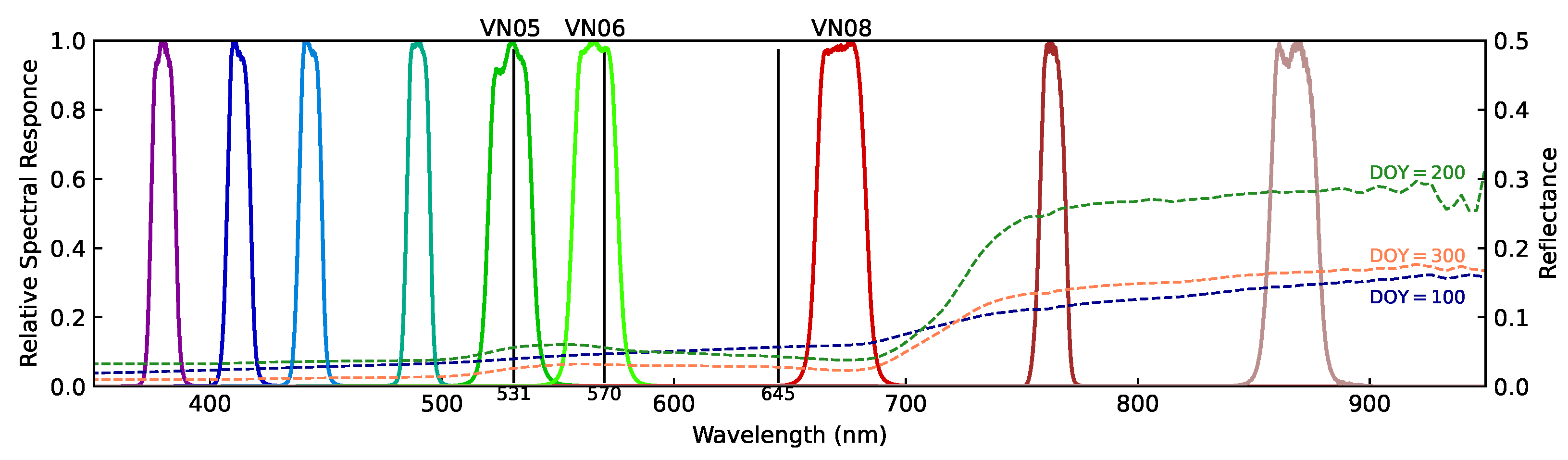
| Band | Center Wavelength | Band Width | Saturation Level | Instantaneous Field |
|---|---|---|---|---|
| Number | [nm] | [nm] | [] | of View (IFOV) [m] |
| VN01 | 379.9 | 10.6 | 240–241 | 250 |
| VN02 | 412.3 | 10.3 | 305–318 | 250 |
| VN03 | 443.3 | 10.1 | 457–467 | 250 |
| VN04 | 490.0 | 10.3 | 147–150 | 250 |
| VN05 | 529.7 | 19.1 | 361–364 | 250 |
| VN06 | 566.1 | 19.8 | 95–96 | 250 |
| VN07 | 672.3 | 22.0 | 69–70 | 250 |
| VN08 | 672.4 | 21.9 | 213–217 | 250 |
| VN09 | 763.1 | 11.4 | 351–359 | 250 |
| VN10 | 867.1 | 20.9 | 37–38 | 250 |
| VN11 | 867.4 | 20.8 | 305–306 | 250 |
| Bit Number | Description | Value = 0 | Value = 1 |
|---|---|---|---|
| 0 | No data | No | Yes |
| 1 | Ocean or land | Ocean | Land |
| 2 | Coast | No | Yes |
| 3 | Sun glint | No | Yes |
| 4 | Sun glint | No | Yes |
| 5 | Detection of snow or ice | No | Yes |
| 6 | Cloud by target day estimation | No | Yes |
| 7 | Probably cloud by multi day estimation | No | Yes |
| 8 | Optical thickness | No | Yes |
| 9 | Saturated | No | Yes |
| 10 | The number of bidirectional reflectance factor (BRF) samples | No | Yes |
| 11 | Stray light | No | Yes |
| 12 | Shadow | No | Yes |
| 13 | Detection of cloud or thick aerosol for polarization channels | No | Yes |
| 14 | Recovery of the data with previous days observation (for non-polarization bands) | No | Yes |
| 15 | Recovery of the data with previous days observation (for polarization bands) | No | Yes |
| Site ID | n | r | RMSE | MAE |
|---|---|---|---|---|
| TSE | 84 | () | 0.048 | 0.031 |
| TKY | 40 | () | 0.124 | 0.084 |
| FJY | 146 | () | 0.093 | 0.066 |
| FHK | 65 | () | 0.085 | 0.049 |
| Site ID | n | r | RMSE | MAE |
|---|---|---|---|---|
| TSE | 84 | () | 0.106 | 0.086 |
| TKY | 40 | () | 0.079 | 0.058 |
| FJY | 146 | () | 0.084 | 0.065 |
| FHK | 65 | () | 0.112 | 0.083 |
| Site ID | n | r | RMSE | MAE | |
|---|---|---|---|---|---|
| PRI | TSE | 81 | () | 0.049 | 0.031 |
| TKY | 29 | () | 0.126 | 0.078 | |
| FJY | 115 | () | 0.090 | 0.063 | |
| FHK | 65 | () | 0.085 | 0.049 | |
| CCI | TSE | 81 | () | 0.108 | 0.088 |
| TKY | 29 | () | 0.089 | 0.065 | |
| FJY | 115 | () | 0.084 | 0.064 | |
| FHK | 65 | () | 0.112 | 0.083 |
| Site ID | n | r | RMSE | MAE | |
|---|---|---|---|---|---|
| PRI | TSE | 69 | () | 0.038 | 0.028 |
| TKY | 18 | () | 0.039 | 0.034 | |
| FJY | 120 | () | 0.065 | 0.050 | |
| FHK | 53 | () | 0.045 | 0.034 | |
| CCI | TSE | 69 | () | 0.104 | 0.088 |
| TKY | 18 | () | 0.087 | 0.064 | |
| FJY | 120 | () | 0.071 | 0.058 | |
| FHK | 53 | () | 0.085 | 0.070 |
Publisher’s Note: MDPI stays neutral with regard to jurisdictional claims in published maps and institutional affiliations. |
© 2022 by the authors. Licensee MDPI, Basel, Switzerland. This article is an open access article distributed under the terms and conditions of the Creative Commons Attribution (CC BY) license (https://creativecommons.org/licenses/by/4.0/).
Share and Cite
Sasagawa, T.; Akitsu, T.K.; Ide, R.; Takagi, K.; Takanashi, S.; Nakaji, T.; Nasahara, K.N. Accuracy Assessment of Photochemical Reflectance Index (PRI) and Chlorophyll Carotenoid Index (CCI) Derived from GCOM-C/SGLI with In Situ Data. Remote Sens. 2022, 14, 5352. https://doi.org/10.3390/rs14215352
Sasagawa T, Akitsu TK, Ide R, Takagi K, Takanashi S, Nakaji T, Nasahara KN. Accuracy Assessment of Photochemical Reflectance Index (PRI) and Chlorophyll Carotenoid Index (CCI) Derived from GCOM-C/SGLI with In Situ Data. Remote Sensing. 2022; 14(21):5352. https://doi.org/10.3390/rs14215352
Chicago/Turabian StyleSasagawa, Taiga, Tomoko Kawaguchi Akitsu, Reiko Ide, Kentaro Takagi, Satoru Takanashi, Tatsuro Nakaji, and Kenlo Nishida Nasahara. 2022. "Accuracy Assessment of Photochemical Reflectance Index (PRI) and Chlorophyll Carotenoid Index (CCI) Derived from GCOM-C/SGLI with In Situ Data" Remote Sensing 14, no. 21: 5352. https://doi.org/10.3390/rs14215352
APA StyleSasagawa, T., Akitsu, T. K., Ide, R., Takagi, K., Takanashi, S., Nakaji, T., & Nasahara, K. N. (2022). Accuracy Assessment of Photochemical Reflectance Index (PRI) and Chlorophyll Carotenoid Index (CCI) Derived from GCOM-C/SGLI with In Situ Data. Remote Sensing, 14(21), 5352. https://doi.org/10.3390/rs14215352