Assessing Through-Water Structure-from-Motion Photogrammetry in Gravel-Bed Rivers under Controlled Conditions

Abstract

Structure-from-Motion (SfM) photogrammetry has become a popular solution for three-dimensional topographic data collection in geosciences and can be used for measuring submerged bed surfaces in shallow and clear water systems. However, the performance of through-water SfM photogrammetry has not been fully evaluated for gravel-bed surfaces, which limits its application to the morphodynamics of gravel-bed rivers in both field investigations and flume experiments. In order to evaluate the influence of bed texture, flow rate, ground control point (GCP) layout, and refraction correction (RC) on the measurement quality of through-water SfM photogrammetry, we conducted a series of experiments in a 70 m-long and 7 m-wide flume with a straight artificial channel. Bed surfaces with strongly contrasting textures in two 4 m-long reaches were measured under five constant flow regimes with three GCP layouts, including both dry and underwater GCPs. All the submerged surface models with/without RC were compared with the corresponding dry bed surfaces to quantify their elevation errors. The results illustrated that the poorly sorted gravel-bed led to the better performance of through-water SfM photogrammetry than the bed covered by fine sand. Fine sediment transport caused significant elevation errors, while the static sand dunes and grain clusters did not lead to noticeable errors in the corrected models with dry GCPs. The elevation errors of the submerged models linearly increased with water depth for all the tested conditions of bed textures, GCP layouts, and discharges in the uncorrected models, but the slopes of the increasing relations varied with texture. The use of underwater GCPs made significant improvements to the performance of direct through-water SfM photogrammetry, but counteracted with RC. The corrected models with dry GCPs outperformed the uncorrected ones with underwater GCPs, which could still be used to correct the underestimation in surface elevation caused by RC. Based on the new findings, recommendations for through-water SfM photogrammetry in measuring submerged gravel-bed surfaces were provided.

1. Introduction

High-resolution topography of the bed surface in both field investigations and flume experiments provides fundamental information for the morphodynamics of gravel-bed rivers [1,2,3,4,5]. The evolution of a gravel-bed surface not only influences local hydraulics, sediment availability and transport, and the overall river bed stability [6,7,8,9,10,11], but also affects the longitudinal channel connectivity and habitat diversity that support riverine organisms [12,13,14]. Digital topographic models have been used in analyzing the morphological evolution of the gravel-bed surface [3,7,10,15], and in numerical simulations to visualize the 3D flow structures or particle movements [16,17,18,19].

The structure from motion with multi view stereo (SfM-MVS; together referred to as SfM in this paper) is an established and widely used photogrammetric technique in geosciences that can acquire high-resolution topographic reconstructions with only consumer-grade cameras installed on unmanned aerial vehicles (UAVs) or mobile frames [20,21,22,23]. SfM photogrammetry shows comparable precision to laser scanning, which requires expensive and bulky equipment [24,25,26]. SfM photogrammetry detects and matches features among a sequence of overlapping and offset images of a static subject to estimate a three-dimensional point cloud for the subject’s surface [27,28]. The camera locations and angles are also simultaneously resolved during this reconstruction process [20,21].

There have been increasing applications of SfM photogrammetry in measuring the topography of gravel-bed surfaces in both field investigations with unmanned aerial vehicles [5,20,29] and flume experiments [10,25,30,31,32,33]. SfM photogrammetry is able to measure the underwater bed surface if the water is clean and calm enough to clearly see the bed [34]. When used for reconstructing submerged topographies with cameras located above the water surface, the SfM technique is referred to as through-water SfM photogrammetry [35,36]. However, bed surface elevations derived from through-water SfM photogrammetry are normally higher than the real values owing to light refraction at the water/air interface [34,37,38,39]. Consequently, in most cases SfM photogrammetry is limited in measuring the topographies of the unsubmerged areas in the field [24,40] or the dry bed surface in flume experiments [15,22,31]. Stopping flow in experiments hinders capturing the continuous evolution of bed surfaces during flow processes, and may cause extra morphological variations during the rapid lowering/raising of water level [35].

The adverse effects of refraction on through-water SfM photogrammetry can be reduced by appropriate corrective methods, which are mainly categorized into two approaches: analytical and image-based [41]. The former approach first creates a mesh to simulate the water surface and then corrects the apparent water depths based on the physics of light refraction at the water surface. The corrected elevations of the underwater bed surface are then calculated by subtracting the corrected water depths from the water surface elevations. Woodget et al. [34] corrected submerged bed elevations by multiplying the apparent water depths by 1.34. Dietrich [38] further developed this method by establishing an iterative refraction correction approach that considered multi-angle geometry of SfM, and required camera locations and orientations as inputs. The second approach corrects the refraction effect by reprocessing the radial distance of each pixel based on a provisional but erroneous depth map or digital surface model (DSM) from the typical SfM pipeline, and then new images are constructed and used to calculate a new DSM [41,42,43]. This method is iterative and would be completed until there are no significant differences between the DSMs generated in two successive iterations [43]. However, this method applied the assumption of a horizontal water surface, and hence, has been mainly applied in coastal systems.

The availability of sufficient texture is an important precondition for high-quality reconstructions of underwater bed surfaces using SfM photogrammetry [44]. Both the variation of grain size (fining and coarsening) and the development of bed structures (e.g., pebble clusters, ribs, stone cells, and steps) are common responses of gravel-bed surfaces to flow and sediment supply conditions [7,10,11,45,46], and significantly influence the texture of the bed surface recorded in images. Water depth has also been reported to significantly influence the precision of through-water SfM photogrammetry [36]. Furthermore, the interaction between water and irregular boundaries in gravel-bed rivers results in fluctuating water surfaces [47], which may also affect light refraction. However, knowledge gaps still exist on the performance of through-water SfM under various conditions of bed surface and flow for gravel-bed rivers, as strict controls over bed texture and flow rate are challenging to implement both in the field and in experiments.

Another key issue for through-water SfM is the layout of Ground Control Points (GCPs), which are measured to scale and georeference the 3D point clouds derived by SfM photogrammetry [48,49,50]. For through-water SfM, no consensus has been reached on whether the GCPs should be located underwater or not. Underwater GCPs have been reported to increase the precision of through-water SfM photogrammetry with refraction correction [35]. However, David et al. [36] found that using underwater GCPs without any refraction correction methods achieved better results than corrected bed surface models for shallow waters. Therefore, further tests are needed to explore how to combine dry and underwater GCPs, and how to balance the GCP layout and refraction correction to optimize the performance of through-water SfM photogrammetry.

The objective of our work is to carefully evaluate the performance of through-water SfM photogrammetry in gravel-bed rivers under controlled conditions. We pursue this objective with the specific research question: how do the (i) bed surface texture, (ii) flow rate, (iii) GCP layout, and (iv) refraction correction influence the performance of through-water SfM photogrammetry? To answer this question, a series of flume experiments were conducted in an artificial straight gravel-bed channel with strictly controlled conditions. The channel size was comparable to a small natural stream [5], so that the results could provide insights for not only flume experiments, but also for field investigations using UAV-based through-water SfM photogrammetry. The errors of all the SfM products were quantified and visualized. The influences of bed surface texture and structure, flow rate, and GCP layout were evaluated and discussed, as well as the limitations of this study.

2. Methods

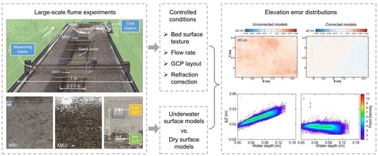
2.1. Flume Equipment

We performed the experiments in a 70-m-long and 7-m-wide flume in the State Key Laboratory of Hydroscience and Engineering at Tsinghua University (Figure 1). Apart from the upper pond, weir, and tailwater pond, the concrete-wall flume had a working distance of 58 m (Figure 1a) that was filled with a sediment mixture comprised of fine sand and gravel. The fine sand was narrowly graded with the D50 (grain size for which 50% of grains are finer than) as 0.36 mm, while the size of the gravels ranged from 9 to 50 mm [51]. The D50 values of seven samples for the gravels in the channel measured by BASEGRAIN [52] were 12–15 mm [53]. The bed was built using both fine sand and gravel, while only the gravel was used to build the banks to form a generally straight channel. The bank top was about 0.5 m higher than the channel bed, and the slopes of both banks were approximately 30° along the channel, resulting in isosceles-trapezoid-like cross-sections. Before this study, over a hundred runs had been conducted with discharges ranging from 10 to 250 L/s in this flume [51]. As a result, the bed surface had reached a relatively stable state in which no significant morphological variation would appear as long as the discharge remained below 120 L/s. The local slope and width of the initial channel bed for this study varied from 0.2–1% and 2–2.5 m along the channel, respectively.

A computer-controlled mobile cart could move transversely on a measuring frame using a laser positioning system with a precision of 2 mm, and could also move longitudinally with the measuring frame from the inlet to the outlet of the channel with the same positioning precision. A Cannon 80D DSLR camera (resolution of 6000 × 4000 pix², 18 mm Cannon lens, FOV = 36.7°) was installed on the mobile cart, approximately 3.4 m above the bed (Figure 1c). The lens of the camera was oriented vertically downwards towards the bed surface, so only nadir pictures were taken and used in this study.

2.2. Experimental Design

To explore the influence of surface texture on through-water SfM photogrammetry, two reaches with contrasting textures were monitored in all the runs in this study (Figure 1a,b). In the upstream monitored reach (MR1, 20.7 m downstream of the channel inlet), fine sand occupied the entire bed surface with only a few gravel particles exposed on the surface. In contrast, in the downstream reach (MR2, 41.7 m downstream of the inlet), the bed surface was mainly covered by gravel with the formation of clusters and small patches of fine sand (Figure 2). The streamwise lengths of the two monitored reaches were both 4 m.

To avoid morphological variations due to fine sediment transport during flow processes, both the bed and banks were cemented (using P. O 42.5 cement) in MR1 (

Table 1. Characteristics of the two monitored reaches.

Reach	Bed Texture	Cement	Analyzed Length (cm)	Analyzed Width (cm)	Grid No.	Bed GCP		Bank GCP
						No.	Mean Height (cm)	No.	Mean Height (cm)
MR1	Fine sand	Bed and bank	360	200	288,000	6	0	6	37
MR2	Gravel	Bank	310	206	255,440	4	7	4	42

). To replicate the morphology of the sand dunes on the initial bed surface, the cement was placed layer by layer, and the thickness of each layer was kept as 3–5 mm. Dark gray sands were added to the top cement layer to increase the richness of surface texture (Figure 2c) and to reduce incorrect feature matching in the SfM workflow [23,25]. The entire cement layer to consolidate the bed had a thickness of 3–4 cm, and was smoothly connected to the uncemented bed surface upstream and downstream of MR1. The bank surfaces were also cemented and the thickness of the cement layer was about 5 cm, without special attention being given to preserving the original morphological features of the banks in MR1. In MR2, only the banks were cemented while the bed was not for two reasons. First, cementing the bed would cause significant losses in the morphological features and grain colors of the gravel-bed surface. Second, the armored gravel-bed surface was stable at, and below discharges of 120 L/s, according to the topographic measurements of the dry bed before and after each run in the pre-experiments.

GCPs that utilized the suggested marker signs by Agisoft Metashape (Figure 2) were installed in the two monitored reaches (Table 1). Each GCP was printed to a 5 mm-thick square PVC panel (10 × 10 cm²). Two sets of GCPs were used in this study: the bed GCPs located on the bed or near bank toes, and the bank GCPs positioned on the banks so that they would remain dry during the experiments. In MR1, six GCPs were flatly embedded in the cement layer of the bed as the bed GCPs (Figure 2a,b). Another six GCP panels were mounted on cement columns as the bank GCPs (Figure 2a), with a mean height of 37 cm above the bed (Table 1). In MR2, eight GCP panels were laid on cement columns on the banks, with four bed GCPs located at the bank toes (Figure 2d,e). The bed GCPs in MR2 were not embedded into the bed, to avoid disturbance of the initial gravel bed surface that had reached equilibrium. The bed and bank GCPs in MR2 had mean heights of 7 cm and 42 cm from the bed surface, respectively (Table 1).

The coordinates of all the GCPs for the two monitored reaches were measured by a total station, with a precision of 2 mm in both the vertical and horizontal directions, fixed near the flume outlet (Figure 1a,b). The location of the total station was set as the origin of the coordinate system used in this study, in which the X direction pointed downstream and the Y direction transversely pointed to the left side of the flume.

2.3. Data Acquisition

Each run was performed with a constant flow rate to maintain a stable water level during measurements. Five discharges of 20, 40, 60, 100, and 120 L/s were tested. After the flow became steady in each run, photographs of MR1 and MR2 were taken by the DSLR camera attached to the mobile cart. When measuring one cross-section, the cart moved stepwise from one side of the measuring frame to the other and stopped for 1 s between consecutive steps. A shutter speed faster than 1/80 s, an aperture of 4–5, and an ISO of 1600–2000 were used to acquire clear and sharp photographs in raw format (i.e., CR2 for Cannon DSLR camera). The time interval between two successive photographs was 3 s. After collecting all the photographs for one cross-section, the measuring frame moved one step downstream to survey the next cross-section. The spatial steps for the camera motion were set as 50 cm in both the streamwise and transverse directions, leading to overlaps of neighboring photographs ≥ 80% (82.7% and 88.5% for streamwise and transverse directions, respectively), which is the requirement for SfM photogrammetry [24,25]. About 3–5 days after the flow was stopped and the water was drained, we collected photographs of the dry bed for the two monitored reaches at the same spatial steps.

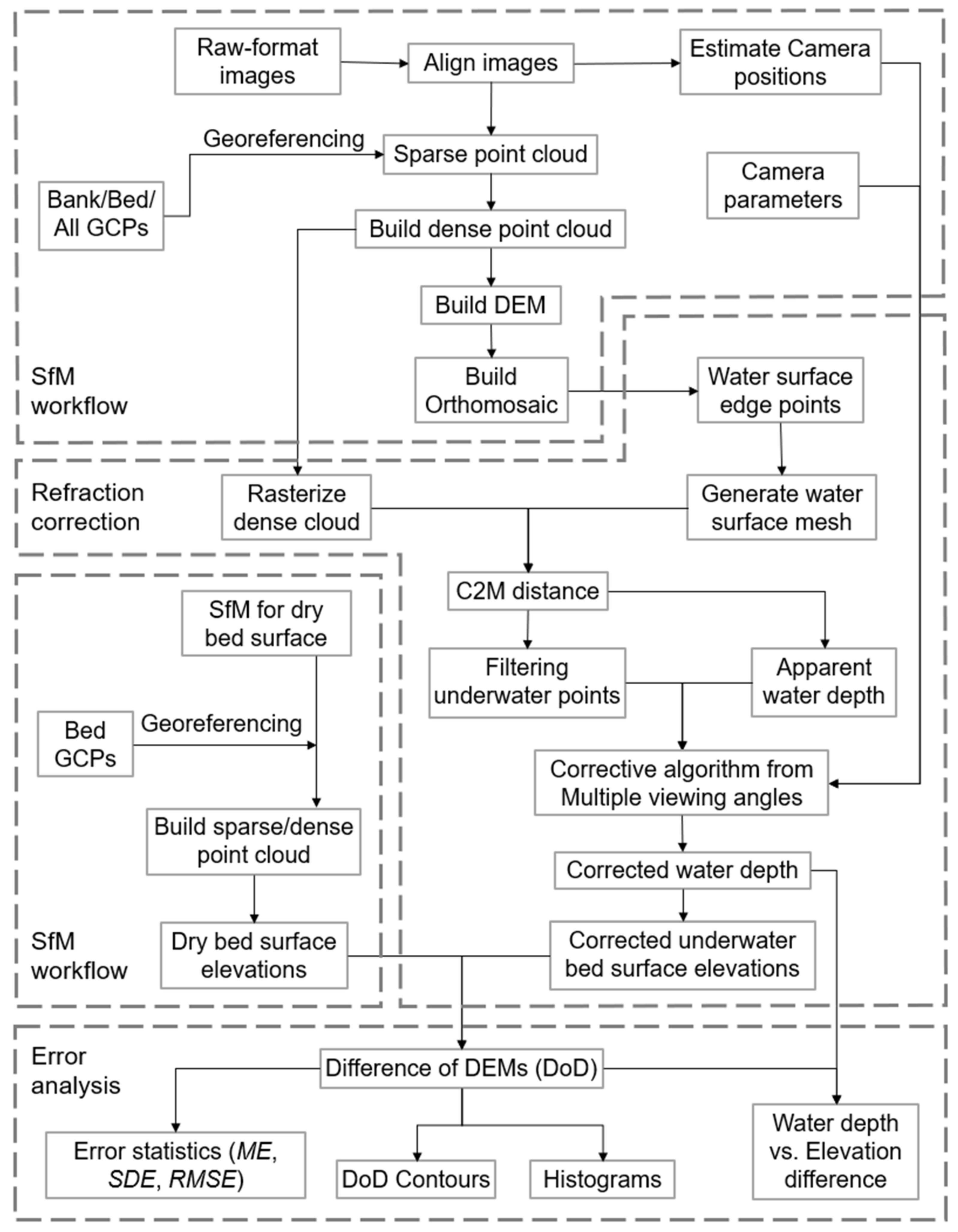
2.4. Data Processing

The commercial software, Agisoft Metashape (Version 1.5.4), was used to generate the 3D topographic models for the bed surfaces under different flow rates and GCP layouts. The raw-format photographs (.CR2 files) were imported into the software to avoid the possible manufacturer-derived on-board image corrections when photographs were saved in JPEG format in the camera [54]. The workflow for SfM reconstruction is presented in Figure 3, and the detailed settings are shown in

Table A1. Settings for the Structure-from-Motion (SfM) and refraction correction workflows.

Workflow	Processing	Setting
SfM	Add photos	Photo quality	>0.5
	Align images	Accuracy	Highest
		Generic preselection	Yes
		Key point limit	40,000
		Tie point limit	4000
		Adaptive camera model fitting	No
		Point colors	3 bands, unit 16
	Georeference to GCPs	Projections	>10
		Error (pix)	<0.5
	Build dense cloud	Quality	High
		Depth filtering	Mild
		Calculate point colors	Yes
	Build DEM	Source data	Dense cloud
		Interpolation	Disabled
		Point classes	All
	Build Orthomosaic	Resolution (m)	0.00064
		Blending mode	Mosaic
		Surface	DEM
		Hole filling	Yes
		Refine seamlines	No
Refraction correction	Rasterize	Grid size	0.005 m
		Grid value	Minimum elevation
		Export	Cloud
	C2M Distance	Max distance	Disabled
		Signed distances	Yes
	Filter submerged area	C2M Distance (m)	≤0
	pyBathySfM	Refractive Index	1.333
		Sensor length (mm)	22.3
		Sensor width (mm)	14.9

in Appendix A.

The refraction correction was mainly performed following the procedures suggested by Dietrich (2017, 2020) as follows. For detailed settings, see Table A1 in Appendix A.

(1) The edges of the water surface were marked in a DOM by points. These edge points were used to generate a Delaunay mesh simulating the water surface in the software CloudCompare (Version 2.10). If anomalous or abrupt changes in elevation along the edges of the water surface existed, the locations of the edge points were adjusted.

(2) The dense cloud was rasterized using a grid size of 5 mm, and the minimum elevation shown in each grid was assigned as the representative elevation [55]. Then, the cloud-to-mesh (C2M) distance between the rasterized dense cloud and the water surface mesh was calculated as the apparent water depth. The submerged points in the dense cloud were filtered based on the combination of the C2M distance and the elevation values. However, some points above the water surface were not removed by this filtering procedure for models with rough water surface edges that led to the incorrect establishment of the water surface mesh near the banks. To solve this problem, a fitting plane was generated for the edge points, and a new C2M distance between this plane and the rasterized dense cloud was used as the second filter for the submerged points (Figure A1 in Appendix A).

(3) The bed surface elevation, apparent water depth, and water surface elevation of each point in the submerged areas were exported to the Python script ‘pyBathySfM’ [55] to correct the apparent water depth of the dense cloud from multiple viewing angles. The camera positions estimated during the SfM workflow and camera parameters (sensor sizes and focal length) were also used by the script. The corrected bed surface elevations were obtained by subtracting the corrected water depths from the water surface elevations.

All the topographic models for dry bed surfaces were obtained using the same SfM settings and rasterization with submerged models, except that only the bed GCPs were employed (Figure 3). The bed GCPs were closer to the surveyed channel bed than the bank GCPs, and hence, showed a stronger control effect on topographic models of the bed (Figure 2). These dry surface models served as reference topographies in quantifying the errors in the through-water SfM models. The differences in DEMs (DoDs) between each submerged model and the corresponding dry bed reconstruction were calculated. The error statistics of these DoDs (i.e., mean error (ME), standard deviation (SDE), and root mean square error (RMSE)) for the analyzed areas (Figure 2b,e; Table 1) were calculated by Equations (1)–(3).

$$ME=\frac{1}{n}{\displaystyle \sum _{i=1}^n{\left(Z_{wet}-Z_{dry}\right)}_i}$$

(1)

$$SDE=\sqrt{\frac{{{\displaystyle \sum _{i=1}^n\left[{\left(Z_{wet}-Z_{dry}\right)}_i-\overline{\left(Z_{wet}-Z_{dry}\right)}\right]}}^2}{n}}$$

(2)

$$RMSE=\sqrt{\frac{{\displaystyle \sum _{i=1}^n{(Z_{wet}-Z_{dry})}^2}}{n}}$$

(3)

The C2M distance between the dry bed surface and water surface mesh was regarded as the true water depth, and was used in analyzing the influence of water depth on through-water SfM photogrammetry (Figure 3). The residual sum of squares (RSS) was calculated for each relation between water depth and elevation difference for a submerged model to quantify the overall deviation of data from the regression for the two monitored reaches.

3. Results

Since the results using all the GCPs generally lie in between the results using the bed or bank GCPs alone, only the results for the underwater models with the bed and bank GCPs are presented in this section, while those for the models using all the GCPs are presented in Figure A2, Figure A3 and Figure A5 in Appendix A.

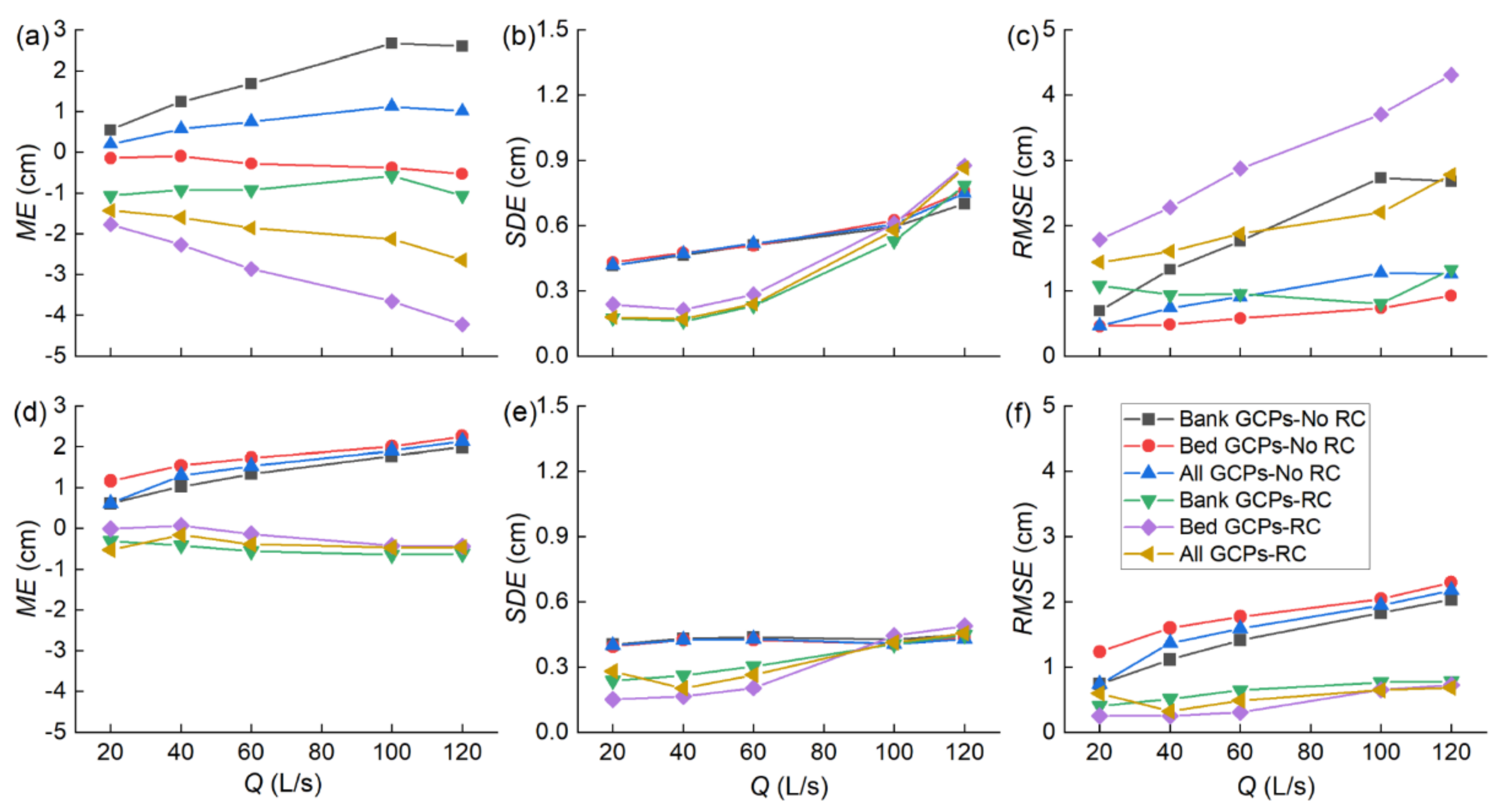
3.1. Error Statistics

Figure 4 presents the error statistics for the through-water SfM models in the two monitored reaches (Figure 2b). For MR1, applying the bank GCPs and all the GCPs led to the overestimation of bed surface elevations (positive ME), while using the bed GCPs resulted in slight underestimations (negative ME) for the uncorrected models. The corrected models showed reduced MEs, whose values generally decreased with flow rate for all the three GCP layouts. The models with bed GCPs showed the highest level of underestimation of bed surface elevations. The SDE for the uncorrected models nearly linearly increased with flow rate, and the three GCP layouts exhibited values close to each other (Figure 4b). Conducting RC resulted in an increase of SDE at the highest discharge, but a decrease of SDE at other flow conditions. The RMSE values of the uncorrected models generally increased with flow for all the three GCP layouts, and the models using the bank and bed GCP layout showed the largest and smallest RMSE values at each flow rate, respectively. Notably, performing RC greatly reduced RMSE values for the models using the bank GCPs, while significantly enhancing the RMSE values when only the bed GCPs were applied (Figure 4c). The RMSE values for the models with all GCPs increased after RC was conducted, meaning that the bed GCPs had a stronger control effect than the bank GCPs on the SfM models for MR1.

As for MR2, the uncorrected models showed positive ME values which increased with flow rate and had a maximum below 2 cm; whereas, the corrected models had generally negative ME values which decreased with discharge for all three GCP layouts and had a minimum higher than −1 cm (Figure 4d). The uncorrected results had SDE values around 0.4 cm at all the discharges (Figure 4e). In comparison, the SDE of the corrected models at Q ≤ 60 L/s decreased, similar to MR1. RMSE values also increased with discharge in MR2, but the models with the bed GCPs showed the largest errors, unlike MR1. RC reduced the RMSE values to lower than 0.8 cm for all three GCP layouts (Figure 4f). The RMSE values were closer to each other for the three GCP layouts than in MR1, indicating that the influence of GCPs on model performance was weaker in MR2 than in MR1.

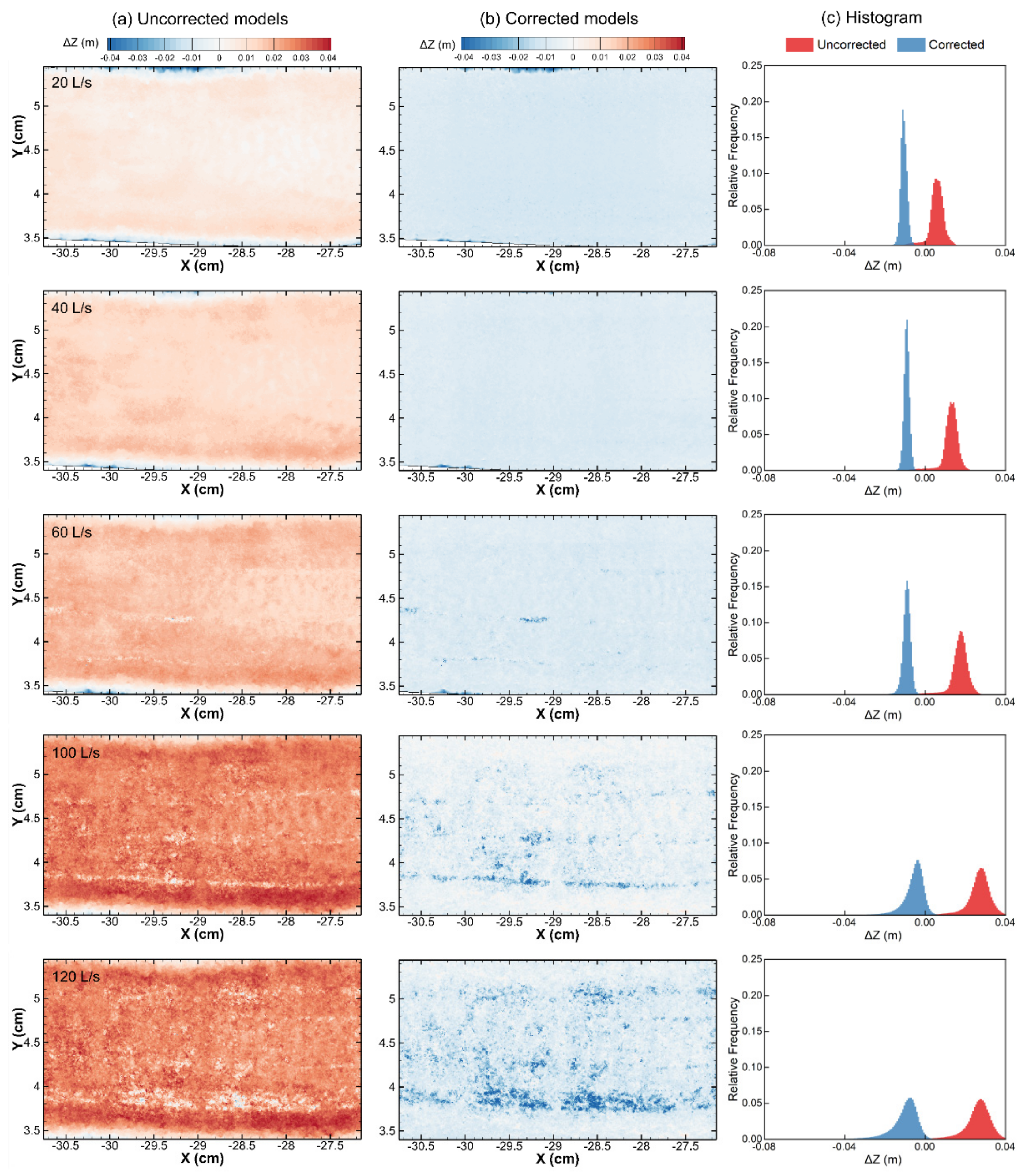
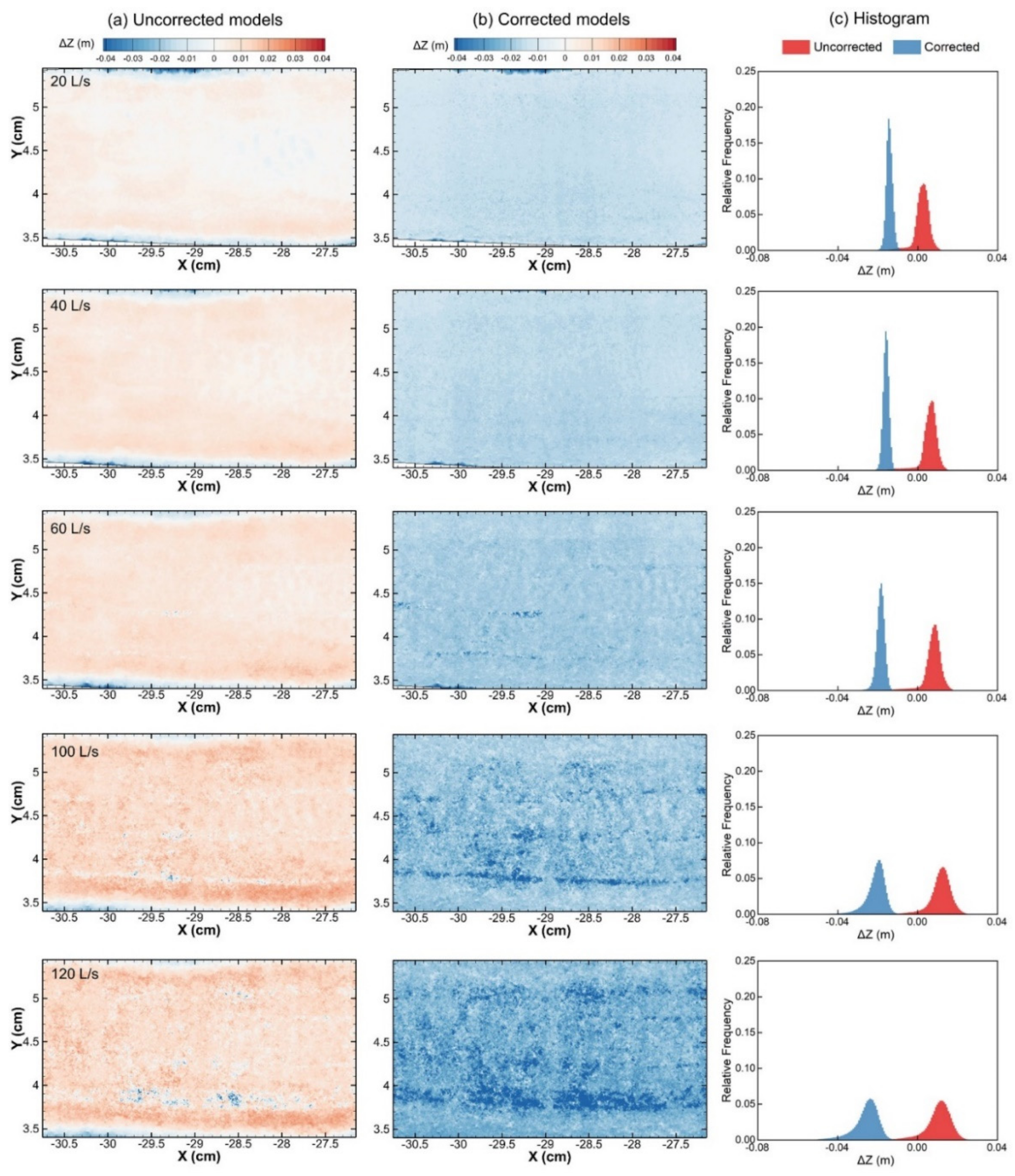
3.2. Error Distributions

3.2.1. MR1

The contours and histograms of the elevation errors for the submerged SfM models with the bank GCP layout are presented in Figure 5, and the key findings were as follows. First, the largest elevation deviations (as overestimations) for the uncorrected SfM models emerged near the bank toes at both sides where the bed elevations were among the lowest in the analyzed area (Figure 2b), especially near the right bank. These elevation differences were greatly reduced by RC. Second, the smallest elevation differences before RC were conducted were located in several streamwise streaks (Figure 5a), where the largest elevation differences (as underestimations) appeared in the corrected models (Figure 5b). These streaks, which were the passages for fine sand transport supplied by the sand deposits in the upstream channel (Figure A4a,b in Appendix A), started to appear after the discharge reached 60 L/s and expanded as flow rate increased. Third, the upstream faces of the sand dunes displayed smaller deviations than the downstream faces. This difference between the upstream and downstream faces was generally eliminated by RC, especially at Q = 100 and 120 L/s. Last, the histograms (Figure 5c) illustrate that RC not only reduced the mean of elevation differences, but also changed their distribution in a way that the elevation differences became more concentrated around the mean at Q ≤ 60 L/s. The distribution shape did not significantly change at Q = 100 and 120 L/s.

The elevation difference distributions for the models with the bed GCPs are displayed in Figure 6. In the uncorrected models, the overestimation of elevations was significantly reduced compared to the uncorrected models that used the bank GCPs (Figure 5a vs. Figure 6a). These models underestimated the elevations in the areas close to the water edges and the areas used for fine sand transportation. The sand dunes remained slightly underestimated in surface elevation under all the flow rates, and the difference between the upstream and downstream faces of the sand dunes again existed in the uncorrected models (Figure 5a). The highest level of underestimation emerged in the streaks with fine sand transportation for both the uncorrected and corrected models. RC resulted in distinct underestimations of surface elevations, and the underestimations intensified with flow increases. The histograms of the corrected models showed lower mean values, but higher data concentrations at Q ≤ 60 L/s, as observed in the models with the bank GCPs. In contrast, the shape of the histograms was nearly unchanged at Q = 100 and 120 L/s after RC was performed (Figure 6c).

3.2.2. MR2

The distributions of surface elevation error for MR2 with only the bank GCPs are exhibited in Figure 7. The uncorrected SfM outputs overestimated the bed surface elevations of the entire surveyed area, and overestimation increased with the flow rate (Figure 7a). Large elevation errors were mainly distributed in two areas with relatively low bed surface elevations (Figure 2e and Figure 7a). Inside these two areas there were small patches showing the lowest errors in the uncorrected models. Subtle transport of fine sands occurred in these small patches, mainly located downstream of the fine sand deposit in MR2 (Figure A4c,d in Appendix A). After RC was performed, most of the surveyed area showed slightly underestimated bed surface elevations. The two lower areas that displayed the large deviations in the uncorrected models still showed the largest errors, but as underestimations in the corrected models (Figure 7b). The overlap in the histograms for the uncorrected and corrected models decreased with discharge increase, and disappeared at Q = 100 and 120 L/s. RC enhanced the data concentration of all the error distributions.

The uncorrected models with bed GCPs showed further overestimated bed elevations than the uncorrected models using the bank GCPs (Figure 7a vs. Figure 8a). There were more areas showing positive elevation differences in the corrected models than the ones using the bank GCPs (Figure 7b and Figure 8b). In the corrected models, the highest underestimation was still located near the patches with sand deposits in the two relatively low areas (Figure 8b). Performing RC resulted in more concentrated distributions of elevation difference at Q ≤ 60 L/s, but a less concentrated distribution at the highest discharge of 120 L/s (Figure 8c).

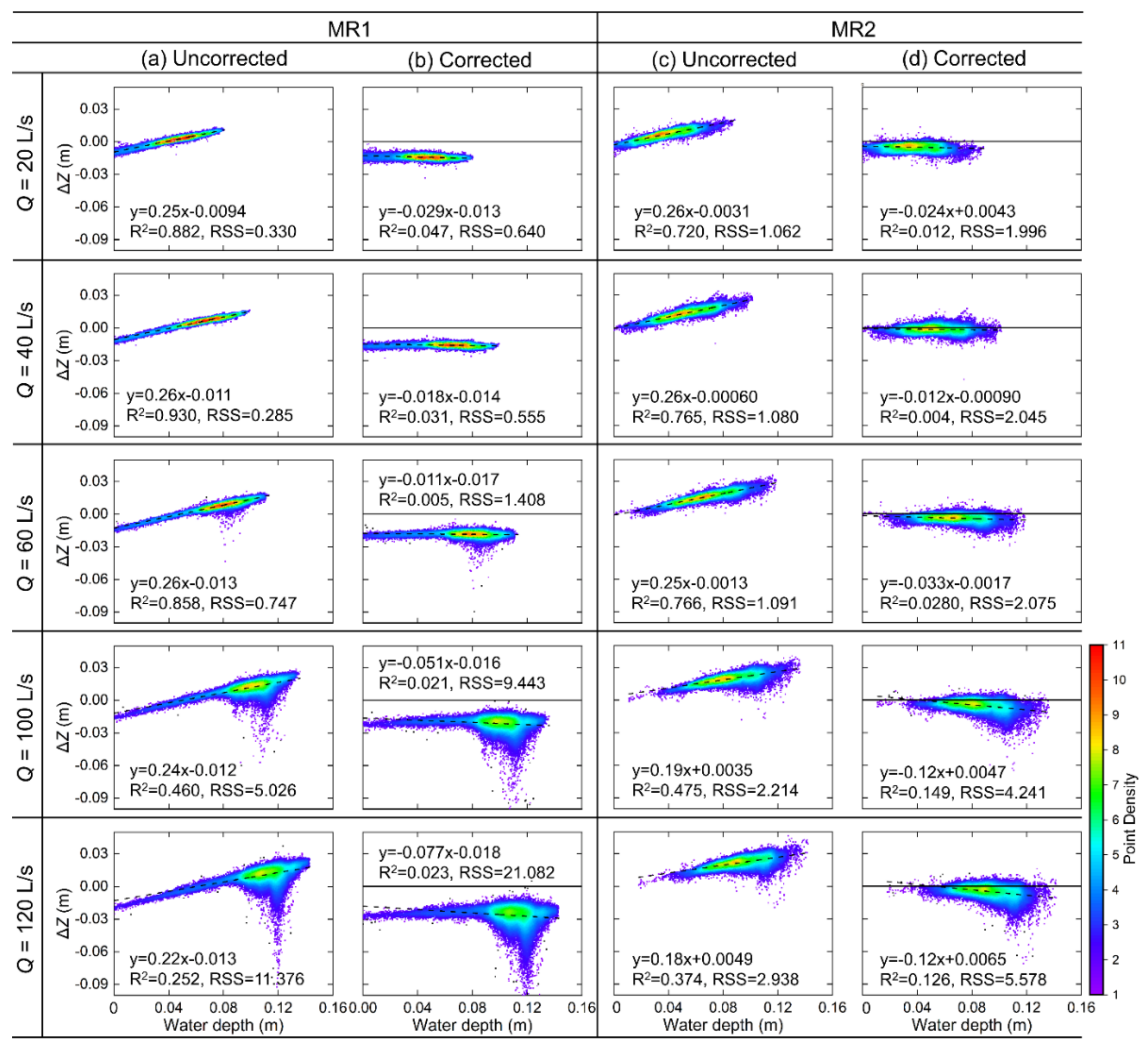
3.3. Error Variation with Water Depth

Figure 9 illustrates the relation between water depth and elevation difference for the submerged models with the bank and bed GCP layouts for MR1. When the bank GCPs were applied, the elevation difference generally increased linearly with water depth for the uncorrected models at all tested flow rates, and the regression slopes were close to each other at Q ≤ 60 L/s (Figure 9a). The RSS value generally increased with discharge, and became over six times larger at Q = 100 and 120 L/s than at Q = 60 L/s. For each flow rate, the data points became particularly scattered as the water depth increased to the range in which the majority of data points were distributed. Distinct deviations from the linear trend also appeared at the water depth range with relatively high point density for Q = 60, 100 and 120 L/s, and the number of deviated data points increased with discharge (Figure 9a). These deviated data points resulted in the decrease of the linear regression slopes and the increase of the RSS. The RC processing significantly reduced the linear regression slopes to around 0 (Figure 9b) but did not eliminate the significant data scattering and deviation. The RSS values of the corrected models were even larger than the uncorrected ones. The interceptions of all the linear regressions for the uncorrected and corrected models were negative, indicating an underestimation of water surface elevations in the submerged models.

When the bed GCP layout was applied, the linearly increasing trend between water depth and elevation error remained for the uncorrected models with similar slopes, but lower interceptions were produced than the uncorrected models using the bank GCPs (Figure 9b vs. Figure 9c), which was related to the lower water surface elevations with the bed GCPs. The significant data deviation from the linear regression still existed at Q ≥ 60 L/s, and the degree of scattering was intensified even further (showing larger RSS values) than the uncorrected models with the bank GCPs. The corrected models showed slightly lower negative slopes of the linear regressions, distinctly lower interceptions, and higher RSS values than the models applying the bank GCPs (Figure 9b vs. Figure 9d).

In MR2, the elevation difference also linearly increased with water depth in the uncorrected models with both bank and bed GCP layouts (Figure 10). RC reduced the regression slopes to be slightly negative, and the regression slope decreased with flow rate in the corrected models with the two GCP layouts. Distinct data deviations from the regression appeared at water depth > 0.1 m in the uncorrected and corrected models at Q ≥ 60 L/s, no matter which GCP layout was applied. The increases of RSS at Q = 100 and 120 L/s from Q ≤ 60 L/s in both the uncorrected and corrected models with the two GCP layouts were smaller in MR2 than those in MR1. The results with the bank and bed GCPs showed two differences (Figure 10a vs. Figure 10c and Figure 10b vs. Figure 10d). First, the data scattering in both uncorrected and corrected models with bank GCPs was reduced at Q = 20 to 60 L/s, but increased at Q = 100 and 120 L/s compared to the models with the bed GCPs. Second, the corrected models with the bed GCPs had more data points showing positive elevation errors. This indicates a lower degree of underestimation in surface elevation than the ones with the bank GCPs, and is consistent with the findings from Figure 7 and Figure 8.

4. Discussions

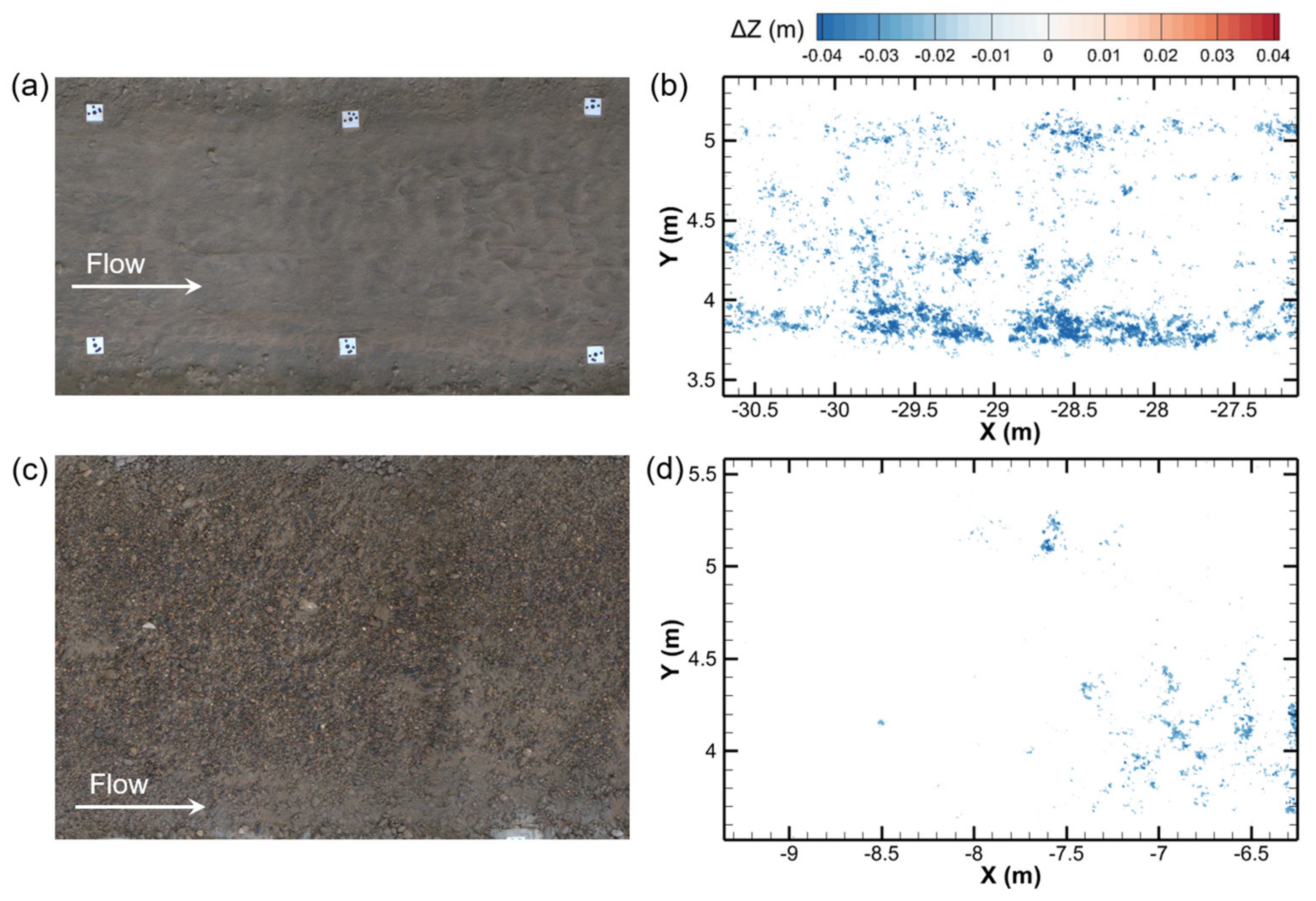
4.1. Influence of Bed Texture

To better present the influence of bed texture on the performance of through-water SfM, only the results with the bank GCP layout for the two monitored reaches were discussed, as the bank GCPs in both reaches had similar distances to the analyzed areas and remained above the water surface. For the uncorrected models, MR1 showed higher ME, SDE, and RMSE values than MR2 at all the flow rates (Figure 4). Another difference lies in that the SDE value increased with flow for the upstream models, while it remained almost unchanged for the downstream ones (Figure 4b,e). After RC was performed, ME turned negative for both the reaches and the models for MR1 showed greater deviation with higher RMSE values (Figure 4c,f). The SDE values for the corrected models for MR2 became slightly higher at Q = 20–60 L/s, while significantly lower at Q = 100–120 L/s than those for the models for MR1. The comparison indicates that the overall performance of through-water SfM was superior in MR2, especially at the two highest tested discharges and for the corrected results.

Different error characteristics were found between the upstream and downstream faces of the dunes in the uncorrected models for MR1 (Figure 5a). The elimination of this difference in the corrected models (Figure 5b) suggests that static dunes have an insignificant influence on through-water SfM outputs if RC is performed. The largest errors (e.g., >0.02 m), concentrated along the streaks for fine sediment transport (Figure A4a,b), mainly resulted from the non-static textures recorded in the successive images. The transport of the fine sediment in MR2, although much lower than in MR1, also resulted in the largest elevation errors at the downstream sides of the sand patches (Figure A4c,d). In contrast, the gravel-bed surface with grain clusters formed around coarse grains did not lead to significant elevation deviations (Figure 7b). These results suggest that static bed structures, such as sand dunes and grain clusters, introduce limited error to through-water SfM products with RC, while varying textures (e.g., due to fine sediment transport) cause significant elevation deviations for a submerged bed surface.

If the areas affected by the fine sediment transport in the corrected models with the bank GCPs for both MR1 and MR2 were excluded (following the threshold method in Section 4.2), the updated statistics of elevation errors show significant improvement in the models for MR1 at Q =100–120 L/s (Figure A6 in Appendix A). Although the SDE values for the models in MR1 and MR2 become similar, the ME and RMSE values of the models for MR2 still outperformed those for MR1. This further indicates that the richer texture of the static gravel-bed results in a more accurate topographic measurement by through-water SfM photogrammetry than the bed covered by sand.

The SfM technique identifies and matches features between the imported images to reconstruct the 3D structure and camera locations in the picture alignment [20,21,24]. The detected features were invariant to image scaling and rotation; partially invariant to illumination conditions, but dependent primarily on image texture and resolution [20,25]. Since the resolution of photographs was fixed in our experiments, the different performances between the two reaches mainly stemmed from the different bed surface textures. The first difference in texture between the sand-bed and gravel-bed lies in that the higher sediment mobility in the former leads to higher variability of the surface texture recorded in the sequential images for SfM photogrammetry. Another difference lies in the static surface. Although dark sands were added to the cemented bed surface in MR1, it was still less textured than the gravel-bed surface, which showed nonuniform grain sizes and colors (Figure 2c,f). The small sand patches that provided contrasting texture with the armored gravel surface (Figure 2d) further enhanced the overall surface texture in MR2.

The distinct elevation errors in both the streaky structures and sand patches also show the potential of through-water SfM photogrammetry to detect fine sediment transport during flow on sand- or gravel-beds. When the transport of fine sediment is low, the passage for sediment transport may have a very limited thickness (e.g., only several millimeters in this study) and show similar colors to the surrounding static sand cover. This reduces the detection efficiency of previous methods that recognized the difference in elevation or color [56]. However, the transport of fine sands might be efficiently detected based on the distinct noises in the DoDs between the through-water SfM models at different times due to the change in texture. Extensive effort (e.g., in determining the optimized time intervals between the successive images captured and exploring whether this method still works during extensive sediment transportation) would still be needed to make this idea feasible and applicable in flume or field investigations.

4.2. Influence of Flow Rate

The primary influence of flow rate increases comes from the increase in water depth. The refraction at the water surface would lead to linearly increased bed elevation errors with the increase in water depth, according to Snell’s law [38]. The linear relations in Figure 9, Figure 10 and Figure A5 are consistent with this theoretical basis, no matter which GCP layout was applied. The refractive index of 1.333 was used in this study and corresponds to the theoretical slope of 0.25 for the linear relations between water depths and elevation differences. Our results matched well with this theoretical prediction at Q = 20–60 L/s for both of the monitored reaches, but showed clear deviation at flows > 60 L/s (Figure 9a and Figure 10a) owing to the large errors related to fine sediment transport, as discussed in Section 4.1.

To better focus on the influence of water depth on the measuring error, we removed the points that had an elevation difference of <−0.02 m, which was the lower boundary of the data points in the high-density range (>5.5) of the corrected models with the bank GCPs for the two surveyed reaches (Figure 9b and Figure 10b;

Table A2. Settings for the analyzed areas and data filtering to remove the distinct errors < −0.02 m in the corrected models with bank ground control points (GCPs).

Sub-Reach	Q (L/s)	Total Grid Number	Removed Point Number	Removed Point Number/Total Grid Number
Upstream	20	278,940	16	0.006%
	40	284,277	5	0.002%
	60	285,885	620	0.217%
	100	287,456	6562	2.283%
	120	287,929	26,063	9.052%
Downstream	20	251,850	8	0.003%
	40	255,440	184	0.072%
	60	255,440	257	0.101%
	100	255,440	3009	1.178%
	120	255,440	3895	1.525%

in Appendix A). The elevation differences of the filtered submerged models at different discharges were combined and plotted against water depth for the two reaches in Figure 11. Clear linear relations still exist in the combined uncorrected results for MR1 and MR2 (Figure 11a,c). This result further confirms the linear influence of water depth on measuring errors of the through-water SfM throughout the water depth range tested in this study. Detectable differences in the linear regression slopes still exist between MR1 and MR2. This suggests that the linear influence of water depth on through-water SfM may be affected by factors such as bed surface texture, other than the water refractive index. David et al. (2021) reported a similar linear relation between water depth and elevation error of through-water SfM using dry GCPs, but with a larger slope of 0.35 in shallow reef and beach environments assuming a refractive index = 1.337 (with a theoretical linear regression slope of 0.252). This mismatch with the theoretical regression slope and our results together suggest that the influence of water depth on through-water SfM cannot simply be decided by the refractive index of the water. Therefore, the simple correction methods for refraction through multiplying the apparent water depths by the refractive index (e.g., in [34,57]) may need further correction to reflect the influence of other factors.

Notably, the interception of the linear regression for the uncorrected models was −8.1 mm for MR1, while it was −1.4 mm for MR2 (Figure 11). This 6.7 mm-difference in interception indicates a higher level of underestimation in water surface elevations in the uncorrected models for MR1. The banks near the water surface edges were more textured in MR2 than in MR1 (Figure 2c,f). This led to more accurate water surface elevations, and consequently, the interception of linear regression for water depth vs. elevation error closer to 0 for MR2. Therefore, it is recommended to keep highly textured banks in flume experiments if through-water SfM is used to collect topographic data.

The increase in flow rate also affected measuring errors through fine sediment transport. The elevation errors in both the streaky structures in MR1 and downstream of the sand patches in MR2 were amplified with flow rate (Figure 5b, Figure 7b and Figure 8b), which resulted in an increased number of deviated data points from the linear relation between water depth and elevation difference (Figure 9 and Figure 10; Figure A5 and Table A2 in Appendix A). The much higher fine sediment transport in MR1 also results in significantly higher data scattering and deviation at the two highest discharges than those in MR2 (Figure 9 and Figure 10). All the above results, together with the discussions in Section 4.1, highlight the need to reduce the adverse effect of fine sediment transport in topographic measurements by through-water SfM. Given that the errors come from the variation of bed texture between the captured images, increasing the temporal resolution of measurement (i.e., shorter time intervals between the successive images with one camera, or simultaneously taking pictures with multiple cameras) may work, and is suggested to reduce the influence of fine sediment transport.

Another influence of the flow increase was the intensification of water surface fluctuation in MR2, which was observed through the glints in the water surface in the two relatively low areas. However, the water surface fluctuation did not result in a significant increase in elevation errors in the corrected models with the bank GCP layout for MR2 (Figure 7b). As recognized in previous studies on through-water SfM photogrammetry, requiring a calm water surface is one of the limitations of this technique [36,38,41]. Our results further reveal that a non-static water surface affects the performance of through-water SfM photogrammetry in a much less noticeable way than fine sediment movement on the bed.

4.3. Influence of GCP Layout and Refraction Correction

The effects of dry (bank) and submerged (bed) GCP layouts were tested in MR1 (Figure 5 and Figure 6). The uncorrected models using the bed GCP layout outperformed those using the bank GCPs in that the overestimation of bed surface elevations owing to refraction did not appear (Figure 6a). In contrast, the corrected models with the bank GCPs showed much smaller deviation in elevations (Figure 5b) than the corrected models with the bed GCPs, which showed distinct underestimation in bed surface elevations (Figure 6b). This comparison suggests that if underwater GCPs are applied in through-water SfM photogrammetry, RC will no longer be needed, which is consistent with the findings by David et al. [36]. If the corrected models with the bank GCPs are compared with the uncorrected models using the bed GCPs, the following differences are found. First, the former showed higher levels of underestimation in bed elevations (with an averaged ME of −0.91 cm; Figure 4a) but higher precision (with lower SDE, especially at Q ≤ 60 L/s; Figure 4b). Second, the histograms were more concentrated to the mean error for the former (Figure 5c and Figure 6c). Third, the area with dunes that is close to the water edges showed lower elevation differences than the surrounding areas in the latter, while such differences did not appear in the corrected models with bank GCPs (Figure 6a). These differences suggest that the corrected models using the dry GCPs may provide a more spatially uniform distribution of elevation errors, but with a larger overall underestimation. The histograms of elevation errors for the submerged models at Q = 20–60 L/s (when the large errors due to fine sediment transport were relatively few) became more concentrated around the mean after RC was performed for all the GCP layouts in both the monitored reaches (Figure 5c, Figure 6c, Figure 7c, Figure 8c, Figure A2c and Figure A3c). This further indicates that RC can improve the spatial uniformity of the elevation errors.

Notably, the difference of 0.92 cm in the ME values between the corrected model with the bank GCPs and the uncorrected model with the bed GCPs was close to the averaged ME values for the corrected models with the bank GCPs under all the tested discharges (Figure 4a). This difference in the ME values at low flows can provide an estimate to correct the overall underestimation of the corrected models with the dry GCPs if both dry and underwater GCPs are applied. After this improvement, the combination of dry GCPs and refraction correction would generate superior results than simply applying underwater GCPs.

Only dry GCPs were installed in MR2, but the bed GCPs were closer to the analyzed area than the bank GCPs. The refraction correction significantly decreased the deviation from the dry bed surface for all the GCP layouts, and the corrected models with the bed GCPs showed the lowest errors (Figure 7 and Figure 8). This suggests that dry GCPs should be placed close to the water surface to improve the performance of through-water SfM photogrammetry with RC. RC also led to the underestimation of surface elevations in the corrected models for MR2, similar to MR1. The underestimation intensified with flow increase in MR2 (Figure 7b and Figure 8b), and the regression slopes of the relations between water depth and elevation difference remained negative for the corrected downstream models using both the bank and bed GCPs at most discharges (Figure 10b,d). Even after removing the large deviations, the corrected models with the bank GCPs still displayed an enlarged underestimation in surface elevation with increasing water depth (Figure 11d). Such underestimation in the corrected models was also observed in the results of Dietrich [38] and Davide et al. [36]. These results together serve as a reminder to users that special attention should be given to topographic measurements by through-water SfM with RC in deep waters of gravel-bed streams.

4.4. Limitations

This study also has several limitations, as discussed below.

• No GCPs were embedded into the bed surface in the downstream monitored reach, which made a direct comparison between the through-water SfM models using the bed GCPs for different bed textures impossible. A possible solution for future research is to first install the GCPs in the gravel bed surface, and then to release flows to the channel until the bed reaches equilibrium.
• Fine sediment transport occurred during the experiments. Since the surveyed reaches only took a small portion of the entire channel, there remained an accessible sediment supply from the upstream uncemented bed to the surveyed areas. As the influence of fine sediment transport is significant to the performance of through-water SfM, the fines should also be carefully controlled in the subsequent experiments on through-water SfM.
• The tested range of flow rate was limited. Although the smallest ratio between channel width and water depth reached 12.5 and 16.7 in MR1 and MR2, respectively, which were comparable or even smaller than previous field tests in gravel-bed rivers [5,34,38,57], the absolute water depths were smaller than most of the field investigations. If more efficient methods are available to keep all the bed materials static at higher flows in future, through-water SfM photogrammetry could be tested in large flumes, such as ours, under flow conditions fully comparable to those in the field.
• Since the camera angle could not be adjusted in our experiments, only nadir images were captured without any oblique imagery. The incorporation of oblique images into nadir-only image blocks has been reported to increase the precision and accuracy of SfM photogrammetry in dry areas [54,58]. Camera calibration [59] was not conducted in the SfM workflow in this study either, as it was difficult to strictly control the parameters in this procedure by the close-sourced algorithm in Metashape. Tests on the effects of oblique images and camera calibration on through-water SfM photogrammetry are still needed to further optimize this technique.

5. Conclusions

In this study we performed flume experiments to evaluate the performance of through-water SfM photogrammetry under different conditions of bed texture, discharge, and GCP layout, as well as with or without refraction correction. This study produced the following main findings.

First, the gravel-bed surface provided richer texture and showed higher accuracy and precision in the through-water SfM reconstruction than the bed surface covered by fine sands. Static sand dunes and gravel-bed surfaces with grain clusters did not cause noticeable measuring errors. In contrast, the streaky structures and small sand patches used as the passage for the transport of fine sediment resulted in the largest elevation error because the texture kept changing during image acquisition. More textured banks improved the elevation accuracy of the water surface mesh, and hence, increased the overall accuracy of through-water SfM models.

Second, the elevation errors in both the uncorrected and corrected through-water SfM models linearly increased with water depth for all the GCP layouts, but the linear relations significantly deviated by the large errors caused by the fine sediment transport at high flow conditions. The slope of the linear relations between water depth and elevation error was determined not only by the refractive index of water, but also by other factors, such as bed texture.

Third, the use of underwater GCPs significantly improved the performance of through-water SfM photogrammetry without performing RC, but resulted in a spatially nonuniform distribution of elevation errors. In contrast, the corrected models using the dry GCPs showed higher precision, but a larger overall underestimation, which could be corrected if underwater GCPs were also used. The dry GCPs closer to the surveyed area provided higher accuracy and precision to the corrected models. The refraction correction method by Dietrich [38,55] efficiently removed the overestimation of the surface elevation in the submerged bed for the gravel-bed surface, but caused a slight underestimation that increased with flow rate.

Our experimental results highlight the feasibility of through-water SfM photogrammetry in measuring submerged gravel-bed surfaces. Based on the findings in this study, the performance of through-water SfM photogrammetry for both field and flume investigations can be improved by the following recommended adjustments.

First, when measuring submerged bed surfaces with rapid morphological variations, a high frequency of image capturing should be applied to keep constant texture recorded in sequential images. Pretests to evaluate the topographic error with regard to image capturing frequency are recommended.

Second, both dry and underwater GCPs are suggested to be installed in the target area. The dry GCPs should be located as close to the water surface as possible. The use of corrected models with dry GCPs is recommended for the reconstruction of the submerged bed, and the uncorrected models with underwater GCPs should also be established to further improve the measuring accuracy.

Third, measures to enrich the texture of the target area (e.g., using multicolored gravels and sands in experiments) are recommended for not only the bed surface, but also the areas near the water surface edges.

References

1. Aberle, J.; Nikora, V. Statistical Properties of Armored Gravel Bed Surfaces. Water Resour. Res. 2006, 42, W11414. [Google Scholar] [CrossRef]
2. Bailly, J.-S.; Coarer, Y.L.; Languille, P.; Stigermark, C.-J.; Allouis, T. Geostatistical Estimations of Bathymetric LiDAR Errors on Rivers. Earth Surf. Proc. Landf. 2010, 35, 1199–1210. [Google Scholar] [CrossRef]
3. Mao, L.; Cooper, J.R.; Frostick, L.E. Grain Size and Topographical Differences between Static and Mobile Armour Layers. Earth Surf. Proc. Landf. 2011, 36, 1321–1334. [Google Scholar] [CrossRef]
4. Brenna, A.; Surian, N.; Mao, L. Response of A Gravel—Bed River to Dam Closure: Insights from Sediment Transport Processes and Channel Morphodynamics. Earth Surf. Proc. Landf. 2020, 45, 756–770. [Google Scholar] [CrossRef]
5. Helm, C.; Hassan, M.A.; Reid, D. Characterization of Morphological Units in a Small, Forested Stream Using Close-Range Remotely Piloted Aircraft Imagery. Earth Surf. Dynam. 2020, 8, 913–929. [Google Scholar] [CrossRef]
6. Montgomery, D.R.; Buffington, J.M. Channel-Reach Morphology in Mountain Drainage Basins. Geol. Soc. Am. Bull. 1997, 109, 596–611. [Google Scholar] [CrossRef]
7. Hassan, M.A.; Church, M. Experiments on Surface Structure and Partial Sediment Transport on a Gravel Bed. Water Resour. Res. 2000, 36, 1885–1895. [Google Scholar] [CrossRef]
8. Strom, K.; Papanicolaou, A.N.; Evangelopoulos, N.; Odeh, M. Microforms in Gravel Bed Rivers: Formation, Disintegration, and Effects on Bedload Transport. J. Hydraul. Eng. 2004, 130, 554–567. [Google Scholar] [CrossRef]
9. Curran, J.C.; Tan, L. Effect of Bed Sand Content on the Turbulent Flows Associated with Clusters on an Armored Gravel Bed Surface. J. Hydraul. Eng. 2014, 140, 137–148. [Google Scholar] [CrossRef]
10. Hassan, M.A.; Saletti, M.; Zhang, C.; Ferrer-Boix, C.; Johnson, J.P.L.; Müller, T.; Flotow, C. Co-Evolution of Coarse Grain Structuring and Bed Roughness in Response to Episodic Sediment Supply in an Experimental Aggrading Channel. Earth Surf. Proc. Landf. 2020, 45, 948–961. [Google Scholar] [CrossRef]
11. Hassan, M.A.; Saletti, M.; Johnson, J.P.L.; Ferrer-Boix, C.; Venditti, J.G.; Church, M. Experimental Insights into the Threshold of Motion in Alluvial Channels: Sediment Supply and Streambed State. J. Geophys. Res.-Earth 2020, 125, e2020JF005736. [Google Scholar] [CrossRef]
12. Wohl, E.; Lane, S.N.; Wilcox, A.C. The Science and Practice of River Restoration. Water Resour. Res. 2015, 51, 5974–5997. [Google Scholar] [CrossRef] [Green Version]
13. Wohl, E. Connectivity in Rivers. Prog. Phys. Geog. 2017, 41, 345–362. [Google Scholar] [CrossRef]
14. Muhlfeld, C.C.; Dauwalter, D.C.; Kovach, R.P.; Kershner, J.L.; Williams, J.E.; Epifanio, J. Trout in Hot Water: A Call for Global Action. Science 2018, 360, 866–867. [Google Scholar] [CrossRef]
15. Wang, J.; Hassan, M.A.; Saletti, M.; Chen, X.; Fu, X.; Zhou, H.; Yang, X. On How Episodic Sediment Supply Influences the Evolution of Channel Morphology, Bedload Transport and Channel Stability in an Experimental Step-Pool Channel. Water Resour. Res. 2021, 57, e2020WR029133. [Google Scholar] [CrossRef]
16. Sandoval, J.; Mignot, E.; Mao, L.; Pastén, P.; Bolster, D.; Escauriaza, C. Field and Numerical Investigation of Transport Mechanisms in a Surface Storage Zone. J. Geophys. Res.-Earth 2019, 124, 938–959. [Google Scholar] [CrossRef] [Green Version]
17. Chen, Y.; DiBiase, R.A.; McCarroll, N.; Liu, X. Quantifying Flow Resistance in Mountain Streams Using Computational Fluid Dynamics Modeling over Structure-from-Motion Photogrammetry-Derived Microtopography. Earth Surf. Proc. Landf. 2019, 44, 1973–1987. [Google Scholar] [CrossRef]
18. Chen, Y.; Bao, J.; Fang, Y.; Perkins, W.A.; Ren, H.; Song, X.; Duan, Z.; Hou, Z.; He, X.; Scheibe, T.D. Modeling of Streamflow in a 30 Km Long Reach Spanning 5 Years Using OpenFOAM 5.x. Geosci. Model Dev. 2022, 15, 2917–2947. [Google Scholar] [CrossRef]
19. Zhang, C.; Xu, Y.; Hassan, M.A.; Xu, M.; He, P. Hybrid Modeling on 3D Hydraulic Features of a Step-Pool Unit. Earth Surf. Dynam. 2022. preprint. [Google Scholar] [CrossRef]
20. Westoby, M.J.; Brasington, J.; Glasser, N.F.; Hambrey, M.J.; Reynolds, J.M. “Structure-from-Motion” Photogrammetry: A Low-Cost, Effective Tool for Geoscience Applications. Geomorphology 2012, 179, 300–314. [Google Scholar] [CrossRef]
21. Eltner, A.; Kaiser, A.; Castillo, C.; Rock, G.; Neugirg, F.; Abellán, A. Image-Based Surface Reconstruction in Geomorphometry—Merits, Limits and Developments. Earth Surf. Dynam. 2016, 4, 359–389. [Google Scholar] [CrossRef] [Green Version]
22. Leduc, P.; Peirce, S.; Ashmore, P. Short Communication: Challenges and Applications of Structure-from-Motion Photogrammetry in a Physical Model of a Braided River. Earth Surf. Dynam. 2019, 7, 97–106. [Google Scholar] [CrossRef] [Green Version]
23. Tmušić, G.; Manfreda, S.; Aasen, H.; James, M.R.; Gonçalves, G.; Ben-Dor, E.; Brook, A.; Polinova, M.; Arranz, J.J.; Mészáros, J.; et al. Current Practices in UAS-Based Environmental Monitoring. Remote Sens. 2020, 12, 1001. [Google Scholar] [CrossRef] [Green Version]
24. Javernick, L.; Brasington, J.; Caruso, B. Modeling the Topography of Shallow Braided Rivers Using Structure-from-Motion Photogrammetry. Geomorphology 2014, 213, 166–182. [Google Scholar] [CrossRef]
25. Morgan, J.A.; Brogan, D.J.; Nelson, P.A. Application of Structure-from-Motion Photogrammetry in Laboratory Flumes. Geomorphology 2017, 276, 125–143. [Google Scholar] [CrossRef] [Green Version]
26. Verma, A.K.; Bourke, M.C. A Method Based on Structure-from-Motion Photogrammetry to Generate Sub-Millimetre-Resolution Digital Elevation Models for Investigating Rock Breakdown Features. Earth Surf. Dynam. 2019, 7, 45–66. [Google Scholar] [CrossRef] [Green Version]
27. Lowe, D.G. Distinctive Image Features from Scale-Invariant Keypoints. Int. J. Comput. Vision 2004, 60, 91–110. [Google Scholar] [CrossRef]
28. James, M.R.; Chandler, J.H.; Eltner, A.; Fraser, C.; Miller, P.E.; Mills, J.P.; Noble, T.; Robson, S.; Lane, S.N. Guidelines on the Use of Structure-from-Motion Photogrammetry in Geomorphic Research. Earth Surf. Proc. Landf. 2019, 44, 2081–2084. [Google Scholar] [CrossRef]
29. Cucchiaro, S.; Cavalli, M.; Vericat, D.; Crema, S.; Llena, M.; Beinat, A.; Marchi, L.; Cazorzi, F. Monitoring Topographic Changes through 4D-Structure-from-Motion Photogrammetry: Application to a Debris-Flow Channel. Environ. Earth Sci. 2018, 77, 632. [Google Scholar] [CrossRef]
30. Zhang, C.; Xu, M.; Hassan, M.A.; Chartrand, S.M.; Wang, Z. Experimental Study on the Stability and Failure of Individual Step-Pool. Geomorphology 2018, 311, 51–62. [Google Scholar] [CrossRef]
31. Zhang, C.; Xu, M.; Hassan, M.A.; Chartrand, S.M.; Wang, Z.; Ma, Z. Experiment on Morphological and Hydraulic Adjustments of Step-Pool Unit to Flow Increase. Earth Surf. Proc. Landf. 2019, 45, 280–294. [Google Scholar] [CrossRef]
32. Ravazzolo, D.; Spreitzer, G.; Friedrich, H.; Tunnicliffe, J. Flume Experiments on the Geomorphic Effects of Large Wood in Gravel-Bed Rivers. In Proceedings of the River Flow 2020, International Conference on Fluvial Hydraulics 2020, Online, 6–17 July 2020; CRC Press: Boca Raton, FL, USA, 2020; pp. 1609–1615. [Google Scholar]
33. Piton, G.; Recking, A.; Coz, J.L.; Bellot, H.; Hauet, A.; Jodeau, M. Reconstructing Depth-Averaged Open-Channel Flows Using Image Velocimetry and Photogrammetry. Water Resour. Res. 2018, 54, 4164–4179. [Google Scholar] [CrossRef]
34. Woodget, A.S.; Carbonneau, P.E.; Visser, F.; Maddock, I.P. Quantifying Submerged Fluvial Topography Using Hyperspatial Resolution UAS Imagery and Structure from Motion Photogrammetry. Earth Surf. Proc. Landf. 2014, 40, 47–64. [Google Scholar] [CrossRef] [Green Version]
35. van Scheltinga, R.C.T.; Coco, G.; Kleinhans, M.G.; Friedrich, H. Observations of Dune Interactions from DEMs Using Through-Water Structure from Motion. Geomorphology 2020, 359, 107126. [Google Scholar] [CrossRef]
36. David, C.G.; Kohl, N.; Casella, E.; Rovere, A.; Ballesteros, P.; Schlurmann, T. Structure-from-Motion on Shallow Reefs and Beaches: Potential and Limitations of Consumer-Grade Drones to Reconstruct Topography and Bathymetry. Coral Reefs 2021, 40, 835–851. [Google Scholar] [CrossRef]
37. Lane, S.N.; Widdison, P.E.; Thomas, R.E.; Ashworth, P.J.; Best, J.L.; Lunt, I.A.; Smith, G.H.S.; Simpson, C.J. Quantification of Braided River Channel Change Using Archival Digital Image Analysis. Earth Surf. Proc. Landf. 2010, 35, 971–985. [Google Scholar] [CrossRef]
38. Dietrich, J.T. Bathymetric Structure-from-Motion: Extracting Shallow Stream Bathymetry from Multi-View Stereo Photogrammetry. Earth Surf. Proc. Landf. 2016, 42, 355–364. [Google Scholar] [CrossRef]
39. Shintani, C.; Fonstad, M.A. Comparing Remote-Sensing Techniques Collecting Bathymetric Data from a Gravel-Bed River. Int. J. Remote Sens. 2017, 38, 2883–2902. [Google Scholar] [CrossRef]
40. Wilson, R.; Harrison, S.; Reynolds, J.; Hubbard, A.; Glasser, N.F.; Wündrich, O.; Anacona, P.I.; Mao, L.; Shannon, S. The 2015 Chileno Valley Glacial Lake Outburst Flood, Patagonia. Geomorphology 2019, 332, 51–65. [Google Scholar] [CrossRef]
41. Agrafiotis, P.; Karantzalos, K.; Georgopoulos, A.; Skarlatos, D. Correcting Image Refraction: Towards Accurate Aerial Image-Based Bathymetry Mapping in Shallow Waters. Remote Sens. 2020, 12, 322. [Google Scholar] [CrossRef]
42. Georgopoulos, A.; Agrafiotis, P. Documentation of a Submerged Monument Using Improved Two Media Techniques. In Proceedings of the 2012 IEEE 18th International Conference on Virtual Systems and Multimedia, Milan, Italy, 2–5 September 2012. [Google Scholar]
43. Skarlatos, D.; Agrafiotis, P. A Novel Iterative Water Refraction Correction Algorithm for Use in Structure from Motion Photogrammetric Pipeline. J. Mar. Sci. Eng. 2018, 6, 77. [Google Scholar] [CrossRef] [Green Version]
44. Mandlburger, G. Through-Water Dense Image Matching for Shallow Water Bathymetry. Photogramm. Eng. Remote Sens. 2019, 85, 445–455. [Google Scholar] [CrossRef]
45. Dietrich, W.E.; Kirchner, J.W.; Ikeda, H.; Iseya, F. Sediment Supply and the Development of the Coarse Surface Layer in Gravel-Bedded Rivers. Nature 1989, 340, 215–217. [Google Scholar] [CrossRef]
46. Weichert, R.B.; Bezzola, G.R.; Minor, H.-E. Bed Morphology and Generation of Step-Pool Channels. Earth Surf. Proc. Landf. 2008, 33, 1678–1692. [Google Scholar] [CrossRef]
47. Roy, A.G.; Buffin-Blanger, T.; Lamarre, H.; Kirkbride, A.D. Size, Shape and Dynamics of Large-Scale Turbulent Flow Structures in a Gravel-Bed River. J. Fluid Mech. 2004, 500, 1–27. [Google Scholar] [CrossRef] [Green Version]
48. James, M.R.; Robson, S.; dOleire-Oltmanns, S.; Niethammer, U. Optimising UAV Topographic Surveys Processed with Structure-from-Motion: Ground Control Quality, Quantity and Bundle Adjustment. Geomorphology 2017, 280, 51–66. [Google Scholar] [CrossRef] [Green Version]
49. Forlani, G.; Dall’Asta, E.; Diotri, F.; di Cella, U.M.; Roncella, R.; Santise, M. Quality Assessment of DSMs Produced from UAV Flights Georeferenced with On-Board RTK Positioning. Remote Sens. 2018, 10, 311. [Google Scholar] [CrossRef] [Green Version]
50. Manfreda, S.; Dvorak, P.; Mullerova, J.; Herban, S.; Vuono, P.; Justel, J.A.; Perks, M. Assessing the Accuracy of Digital Surface Models Derived from Optical Imagery Acquired with Unmanned Aerial Systems. Drones 2019, 3, 15. [Google Scholar] [CrossRef] [Green Version]
51. Chen, Y. Study of the Resistance Structure of Gravel Bed in Wide Shallow Channel. Master’s Thesis, Tsinghua University, Beijing, China, 2015. (In Chinese with English abstract). [Google Scholar]
52. Detert, M.; Weitbrecht, V. Automatic Object Detection to Analyze the Geometry of Gravel Grains—A Free Stand-Alone Tool. In Proceedings of the River Flow 2012, International Conference on Fluvial Hydraulics 2012, San José, CA, USA, 5–7 September 2012; CRC Press: Boca Raton, FL, USA, 2012; pp. 595–600. [Google Scholar]
53. Huang, K.; Zhang, C.; Xu, M.; Lin, Y. Application study on the automated grain sizing based on BASEGRAIN software. J. Sediment Res. 2020, 45, 44–51, (In Chinese with English abstract). [Google Scholar] [CrossRef]
54. James, M.R.; Antoniazza, G.; Robson, S.; Lane, S.N. Mitigating Systematic Error in Topographic Models for Geomorphic Change Detection: Accuracy, Precision and Considerations beyond off-Nadir Imagery. Earth Surf. Proc. Landf. 2020, 45, 2251–2271. [Google Scholar] [CrossRef]
55. Dietrich, J.T. Py\_sfm\_depth Homepage. Available online: https://www.geojames.github.io/py_sfm_depth (accessed on 3 June 2020).
56. Wang, H.; Zhong, Q.; Wang, X.; Li, D. Quantitative Characterization of Streaky Structures in Open-Channel Flows. J. Hydraul. Eng. 2017, 143, 04017040. [Google Scholar] [CrossRef]
57. Detert, M.; Johnson, E.D.; Weitbrecht, V. Proof-of-Concept for Low-Cost and Non-Contact Synoptic Airborne River Flow Measurements. Int. J. Remote Sens. 2017, 38, 2780–2807. [Google Scholar] [CrossRef]
58. Nesbit, P.; Hugenholtz, C. Enhancing UAV–SfM 3D Model Accuracy in High-Relief Landscapes by Incorporating Oblique Images. Remote Sens. 2019, 11, 239. [Google Scholar] [CrossRef]
59. Shortis, M. Camera Calibration Techniques for Accurate Measurement Underwater. In 3D Recording and Interpretation for Maritime Archaeology; Coastal Research Library, McCarthy, J., Benjamin, J., Winton, T., van Duivenvoorde, W., Eds.; Springer: Cham, Switzerland, 2019; Volume 31, pp. 11–28. [Google Scholar]
Figure 1. (a) Planform scheme of the flume system in which the monitored reach 1 and 2 (MR1 and MR2) are marked by black dashed squares (unit: meter); (b) photograph of the flume with MR1 and MR2 marked by green dashed squares; (c) photograph of the measuring frame and mobile cart.
Remotesensing 14 05351 g001
Figure 2. Layouts of the ground control points (GCPs). Panels (a,b) exhibit the GCP locations in the digital orthophotomosaic (DOM) and digital elevation model (DEM) of MR1, respectively, with the area of sand dunes marked in (a). Panel (c) presents a close photograph of the bed texture (with sand dunes) in MR1. Panels (d,e) show the GCP locations in the DOM and DEM of MR2, respectively, with the sand patches marked in (d), and panel (f) shows a photograph of the bed surface around D4 in MR2. The dashed squares in (b,e) depict the area analyzed in the results section, and Zdry indicates the bed elevations measured under dry bed conditions. All the GCPs shown in panels (c,f) had a side length of 10 cm.
Remotesensing 14 05351 g002
Figure 3. Schematic workflow of data processing in this study.
Remotesensing 14 05351 g003
Figure 4. Error statistics for the submerged models with/without refraction correction (RC) for MR1 (ac) and MR2 (df). Mean error (ME) is an indicator for accuracy; standard deviation (SDE) is an indicator for precision; and root mean square error (RMSE) illustrates deviation from the dry bed surface. All the statistics were calculated based on the DoDs between the submerged models and dry models.
Remotesensing 14 05351 g004
Figure 5. The contours and histograms of elevation errors for the through-water SfM models using the bank GCPs for MR1: (a) uncorrected models; (b) corrected models; (c) histograms. Flow goes from the left to the right.
Remotesensing 14 05351 g005
Figure 6. The contours and histograms of elevation errors for the through-water SfM models using the bed GCPs for MR1: (a) uncorrected models; (b) corrected models; (c) histograms. Flow goes from the left to the right.
Remotesensing 14 05351 g006
Figure 7. The contours and histograms of elevation errors for the through-water SfM models using the bank GCPs for MR2: (a) uncorrected models; (b) corrected models; (c) histograms. Flow goes from the left to the right. The two relatively low areas are marked by green dashed lines in (a) at Q = 120 L/s.
Remotesensing 14 05351 g007
Figure 8. The contours and histograms of elevation errors for the through-water SfM models using the bed GCPs for MR2: (a) uncorrected models; (b) corrected models; (c) histograms. Flow goes from the left to the right.
Remotesensing 14 05351 g008
Figure 9. Relations between water depth and elevation error for MR1: (a,b) for the uncorrected and corrected models with the bank GCPs, respectively; (c,d) for the uncorrected and corrected models with the bed GCPs, respectively. Point density refers to the point number at each plotted point location. Linear regression for each relation is presented with the regression equation, R-square, and residual sum of squares (RSS).
Remotesensing 14 05351 g009
Figure 10. Relations between water depth and elevation error for MR2: (a,b) for the uncorrected and corrected models with the bank GCPs, respectively; (c,d) for the uncorrected and corrected models with the bed GCPs, respectively. Linear regression for each relation is presented with the regression equation, R-square, and residual sum of squares (RSS).
Remotesensing 14 05351 g010
Figure 11. Relations between water depth and elevation differences for the combined results: (a) uncorrected models for MR1; (b) corrected models for MR1; (c) uncorrected models for MR2; and (d) corrected models for MR2. All the through-water SfM models used the bank GCP layout, and the points with elevation errors < −0.02 m in the corrected models were removed. The linear regression for each relation is presented with the regression equation, R-square, and residual sum of squares (RSS).
Remotesensing 14 05351 g011