Orographic Construction of a Numerical Weather Prediction Spectral Model Based on ASTER Data and Its Application to Simulation of the Henan 20·7 Extreme Rainfall Event

Abstract

Numerical weather prediction (NWP) has become an important method of predicting extreme weather events, but orography is one of the key factors affecting the performance of NWPs. In this paper, based on Advanced Spaceborne Thermal Emission and Reflection Radiometer (ASTER) elevation data, a method for constructing a global orographic dataset suitable for NWP spectral models is investigated. The Yin-He global spectrum model (YHGSM) is used to simulate the early and peak periods of the extreme rainfall event on 20 July 2021 in Henan Province, China, and the heavy rain in Beijing in order to verify the effectiveness and superiority of the proposed orographic construction method. It is demonstrated that in a few cases the direct two-dimensional filter can sometimes simulate more intense rainfall, but in general, the bidirectional one-dimensional filter is better than the direct two-dimensional filter in orographic processing, and the bidirectional one-dimensional filter can filter out more of the small-scale orographic information. The effect of the higher orographic resolution before conversion to spectral space is not very obvious, but it is demonstrated that the simulation results are better for the heavy-rainfall level. In conclusion, in most cases, the simulations conducted using the new global orographic dataset based on ASTER data are better than those obtained using the model’s original orography, especially for torrential and extreme rainfall. These conclusions provide a reference for future predictions of and research on extreme rainfall events.

1. Introduction

Under global climate change, extreme weather events are occurring with increasing frequency [1]. Extreme weather events not only cause great damage to the environment but also pose a great threat to the property and lives of local residents. From 17 to 21 July 2021, Henan Province in China experienced extreme rainfall. On 20 July 2021, Zhengzhou received 201.9 mm of rainfall in one hour (a national record in China), and the total rainfall of the event was 720 mm, exceeding the annual average. This extreme rainfall event resulted in more than 302 deaths and reported economic losses of $17.7 billion [2,3]. It has attracted a great deal of attention in China and abroad. At present, numerical weather prediction (NWP) models are one of the main means of predicting extreme weather events. Orography is one of the key factors affecting the prediction accuracy of NWP models [4,5]. Orography of different scales plays an important role in atmospheric movement, and it also has an important influence on the movement and evolution of weather systems. When air flows over uneven mountains, the orography causes the air to climb and bypass the mountains, which affects the energy transfer and budget of the atmosphere through its thermodynamic effects [6]. In NWP models, it is crucial to accurately represent the orographic effects in the prediction of extreme weather events. Among NWP models, the global spectral model has many advantages, such as high precision, good stability, simple application, and a prominent program [7]. It has been widely used in theoretical research and forecasting. The NWP spectral model is mainly used to simulate the global circulation. The relevant orographic datasets in the spectral models must cover the entire Earth. In recent years, relatively few studies have been conducted on the orographic structure in NWP spectral models. Therefore, it is a new and meaningful challenge to acquire and produce high-precision orographic datasets for NWP spectral models in order to accurately describe the orographic effects and improve the ability to predict extreme weather events globally.

In the 1950s, the average orographic height was estimated by eye, and the navigation charts were incomplete. The first orographic dataset used in an NWP model was read from aeronautical orographic charts [8]. With the continuous development of satellite and remote sensing technology, various digital versions of high-resolution orographic data have been generated [9,10,11,12]. For high-resolution orographic elevation data, the NWP cannot describe the actual impact of the relatively small-scale orography on the atmosphere [13,14,15,16]. The impact of this small-scale orography is usually represented by a parameterization scheme. For example, in general, the orographic effect below the 5 km scale is represented by the turbulent orographic form drag (TOFD) parameterization scheme. The orographic effect from 5 km to the model grid distance scale is characterized by the orographic gravity wave drag (OGWD) parameterization scheme [6]. If these small-scale orographic features exist in the NWP model’s dynamic, the model cannot correctly represent these small-scale orographic effects, and the small-scale orographic features will have a serious negative impact on the performance of the NWP model [15]. In addition, sharp orography can also cause the Gibbs phenomenon in the spectral mode [17], which is mainly manifested as overshooting and undershooting around jump discontinuities, which has adverse effects on the determination of the airflow path [18]. Therefore, in order to ensure the computational stability and accurate prediction of NWP models, it is necessary to perform smoothing and filtering operations on the orography to filter out these small-scale orographic features that are harmful to the NWP. There have been some studies on orographic processing in NWP [19,20,21,22]. However, most of these studies remain in the last century. Davies and Brown [15] also suggested using smoothing and filtering schemes to filter out some scales of orographic features. Webster et al. [23] applied the filter given by Raymond [24] to the Met Office Unified Model (UM) as a orographic filtering scheme and found it could improve or eliminate excessive wind speeds at some grid points. Rutt et al. [25] proposed a novel and very flexible variational method for orography smoothing and validated its performance in numerical models. Later, Wang et al. [26] also designed a filter coupled by different one-dimensional, high-order, low-pass implicit tangent filters, which can selectively filter noise of different scales caused by orographic slope. If the orographic processing method is not proper, it often cannot reflect the real orography well, or the smoothing effect is lost because the waves that adverse to the performance of an NWP cannot be filtered out [26]. The purpose of orographic processing is to achieve a reasonable compromise between maintaining the authenticity of the orography and increasing the smoothness of the orography.

A digital elevation model (DEM) is a digitized raster representation of the surface orography. In this study, the construction of new orographic data was carried out based on the Yin-He global spectrum model (YHGSM). The model’s original orography is mainly based on the Shuttle Radar Topography Mission (SRTM) data. The National Aeronautics and Space Administration (NASA) and National Geospatial-Intelligence Agency (NGA) opened the first version of SRTM dataset in 2003 [10,11]. The Advanced Spaceborne Thermal Emission and Reflection Radiometer (ASTER) is a 14-channel imaging instrument that has been operating on the NASA’s Terra satellite. The ASTER project is jointly researched by the Ministry of Economy, Trade and Industry (METI), and NASA, with METI providing the instruments and NASA providing the spacecraft and launch vehicle. The joint US/Japan ASTER scientific team is responsible for scheduling data acquisition, maintaining instrument calibration, and archiving and distributing data to users. In 2009, the ASTER project released the first high spatial resolution global DEM (GDEM) available to all users. In the GDEM V2 released in 2011, the GDEM was improved to reduce artifacts. In addition, higher resolution correlation was conducted, and additional scenes were added to fill in holes. In August 2019, the ASTER scientific team released the GDEM V3. This most recent version of the GDEM was processed using new custom software to eliminate most of the artifacts [27,28]. Nikolakopoulos [9,10] compared the ASTER GDEM dataset with GTOPO30, SRTM to prove the accuracy and superiority of the ASTER GDEM dataset. Based on the latest version of ASTER GDEM, this study developed a new orographic construction technique to produce a global orographic dataset. After a series of processing operations, a basic orographic dataset suitable for use in the NWP global spectral model was produced. The YHGSM and the new global orographic dataset were used to simulate the extreme rainfall event in Henan, China, on 20 July 2021. The results of this study provide a reference for the selection of orography datasets when using NWP spectrum models to predict extreme weather in the future. The rest of this paper is organized as follows: Section 2 introduces the NWP model used in the study, the design of the filters, and the processing steps of the orographic data. Section 3 analyzes the simulation and enhancement of heavy rain in Henan using the newly fabricated orography. Section 4 discusses the characteristics of the different filters and the advantages of the newly made orography. Section 5 gives the summaries and conclusions.

2. Materials and Methods

2.1. The Yin-He Global Spectrum Model

The YHGSM is a global spectral numerical weather prediction model developed by the National University of Defense Technology (NUDT). The YHGSM adopts a global spectral dynamic core, which satisfies the dry-mass conservation principle [29], and the fast spherical harmonic transform algorithm developed by Yin et al. [30]. In the horizontal direction, a spherical harmonic spectrum expansion based on trigonometric truncation (the maximum truncated wave number is 1279) and a linear Gaussian reduced mesh are used. In the vertical direction, a finite element discretization based on a cubic spline and the terrain following pressure-based coordinates are used. There are a total of 137 vertical layers. The time step is 600 s. The parameterized physical and chemical processes include radiation, turbulence, subgrid orographic drag, cumulus convection, large-scale rainfall, land surface processes, and methane and ozone chemistry [31]. Additional details about the YHGSM have been reported in previous studies [32,33,34,35].

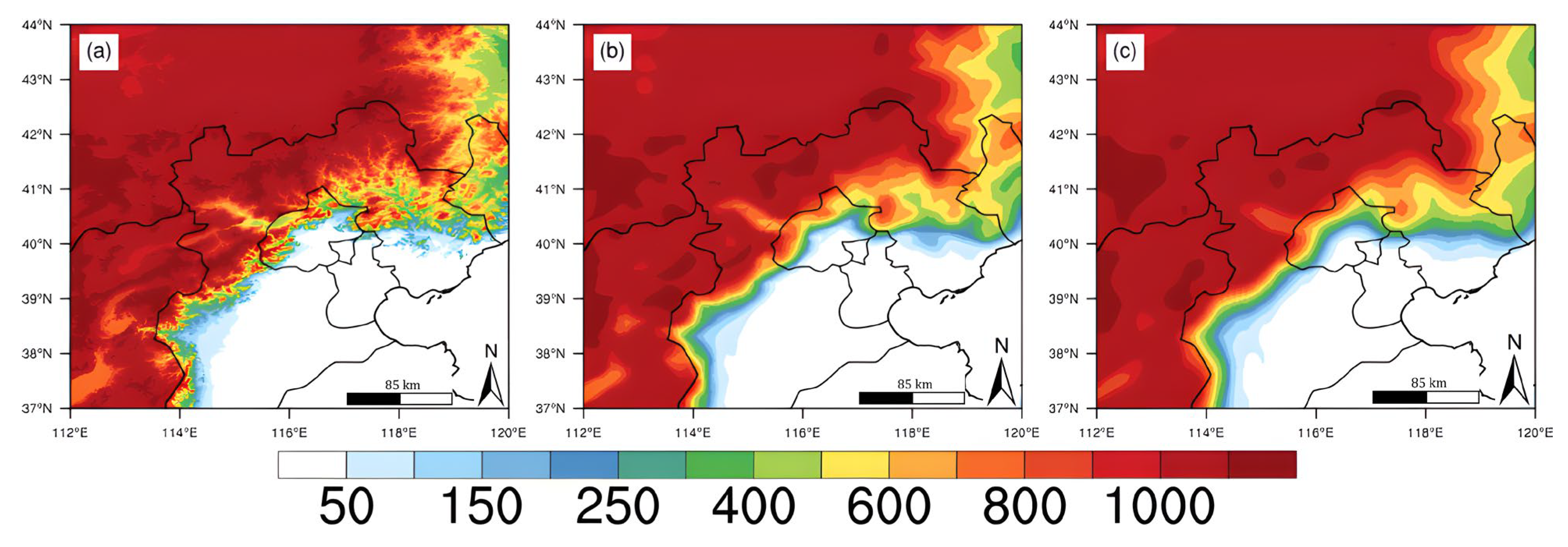
2.2. Orographic Data and Filter

The latitude and longitude resolution of the ASTER GDEM V3 data is 1 arc-second (about 30 m), and the vertical accuracy is about 10 m. The data were tiled as more than 22,000 1×1° latitude/longitude files, each of which was accompanied by a quality file. The dataset covers the Earth’s surface from 83° N to 83° S. To construct a complete global orographic dataset, another DEM (i.e., GTOPO30) was used in the areas not covered by the ASTER GDEM, with a horizontal resolution of 30 arc-seconds (about 1 km). The DEM was derived from multiple raster and vector sources of orographic information. Before processing the orographic data, the datasets with different resolutions needed to be interpolated to the same resolution; that is, the ASTER GDEM dataset with a resolution of 1 arc-second resolution was interpolated to a latitude and longitude grid with a resolution of 30 arc-second. Then, it was combined with the GTOPO30 data at a resolution of 30 arc-seconds to form the initial global orographic dataset.

In order to optimize the description of orographic effects in the model dynamics part, it is necessary to filter out the orographic information of scales that adverse to the performance of the NWP model dynamics. These orographic effects that cannot be described by NWP model dynamics should be described in the NWP physical process parameterization schemes. When filtering the orography in grid-point space, the idea of Gaussian filtering was adopted: that is, the grid point closer to the center has a larger weight value. In order to better filter out small-scale orographic features that cannot be described by the NWP model’s dynamic, that is, orographic features below 5 km scale (described by the TOFD parameterization scheme) and orographic features from 5 km scale to model grid scale (described by the OGWD parameterization scheme), this study mainly used two types of filters, namely, a bidirectional one-dimensional filter and a direct two-dimensional filter. Bidirectional one-dimensional filtering is divided into two steps. First, the latitude (longitude) direction is filtered, and then the longitude (latitude) direction is filtered. Since the orographic dataset is contains equal latitude and longitude grids rather than equal distance grids, a bidirectional one-dimensional filter can easily control the consistency of the filtering scales on the global scale.

$$\begin{array}{l}{w}_{i,j}=\frac{G_1}{P_1^{i\left(or j\right)}}\hspace{1em}\hspace{1em}\hspace{1em}\hspace{1em}\left|r\right|\le \frac{\gamma }{2}-\delta \\ w_{i,j}=\frac{G_2}{P_2^{i\left(or j\right)}}\hspace{1em}\hspace{1em}\frac{\gamma }{2}-\delta <\left|r\right|\le \frac{\gamma }{2}\\ w_{i,j}=\frac{G_2}{P_2^{i\left(or j\right)}}\hspace{1em}\hspace{1em}\frac{\gamma }{2}<\left|r\right|\le \frac{\gamma }{2}+\delta .\\ w_{i,j}=0 \hspace{1em}\hspace{1em}\hspace{1em}\hspace{1em}\hspace{1em}\hspace{1em}\left|r\right|>\frac{\gamma }{2}+\delta \end{array}$$

(1)

In Equation (1), $w_{i,j}$ is the filtering weight of grid point $\left(i, j\right)$, $r$ is the distance from grid point $\left(i, j\right)$ to the central grid point, and γ and δ are constants selected according to the filtering scale, called filter scale and edge scale, respectively. $P_1$, $P_2$, and $P_3$ are the number of grid points whose distances from the center grid point are within $\left|r\right|\le \frac{\gamma }{2}-\delta$, $\frac{\gamma }{2}-\delta <\left|r\right|\le \frac{\gamma }{2}$, and $\frac{\gamma }{2}<\left|r\right|\le \frac{\gamma }{2}+\delta$, respectively. $G_1$, $G_2$, and $G_3$ are the total weights of the three types of points, respectively, and their values are determined by the proportion of the area under the one-dimensional Gaussian distribution function curve to the total area (Figure 1). The one-dimensional Gaussian distribution function is

$$G\left(x\right)=\frac{1}{\sqrt{2\pi }\sigma }{e}^{-\frac{{\left(x-\mu \right)}^2}{2{\sigma }^2}}$$

(2)

where $\mu$ is the location parameter of the Gaussian distribution, which was set to 0 in this study. $\sigma$ describes the degree of dispersion of the data distribution, where $\sigma =\frac{\frac{\gamma }{2}+\delta }{2}$, and it is assumed that the grid points other than $2\sigma$ no longer affect the central point. Figure 1 shows the curve distribution of Equation (2). The proportions of the area under the line for $\left|x\right|\le \frac{\gamma }{2}-\delta$, $\frac{\gamma }{2}-\delta <\left|x\right|\le \frac{\gamma }{2}$, and $\frac{\gamma }{2}<\left|x\right|\le \frac{\gamma }{2}+\delta$ are 63.8%, 25%, and 11.2%, respectively, and thus, $G_1=0.638$, $G_2=0.25$, and $G_3=0.112$. The scale unit of the filter is km, and the resolution unit of the initial global orographic dataset is radians. Therefore, the values of $P_1$, $P_2$, and $P_3$ will change with latitude when filtering in the latitude direction in order to ensure the consistency of the filter scale on the global scale.

The scale unit of the direct two-dimensional filter is the Manhattan distance, so there is no uniform filtering scale across the globe.

$$\begin{array}{l}{w}_{i,j}=\frac{G_1}{P_1 } \hspace{1em}\hspace{1em}\hspace{1em} \left|r\right|\le 1.\\ w_{i,j}=\frac{G_2}{P_1}\hspace{1em}\hspace{1em}1<\left|r\right|\le 2\\ w_{i,j}=\frac{G_3}{P_3}\hspace{1em}\hspace{1em}2<\left|r\right|\le 3.\\ w_{i,j}=0 \hspace{1em}\hspace{1em}\hspace{1em}\hspace{1em} \left|r\right|>3\end{array}$$

(3)

In Equation (3), $r$ is the Manhattan distance from grid point $\left(i, j\right)$ to the central grid point, $G_1$, $G_2$, and $G_3$ remain at the previous values, and $P_1$, $P_2$, and $P_3$ become fixed constants that do not change with latitude. As is shown in Figure 2, $P_1$ is equal to the number of squares with the darkest color, that is, $P_1=5$. $P_3$ is equal to the number of squares with the lightest color, that is, $P_3=12$. $P_2$ is equal to the number of squares in between these two shades, that is, $P_2=8$.

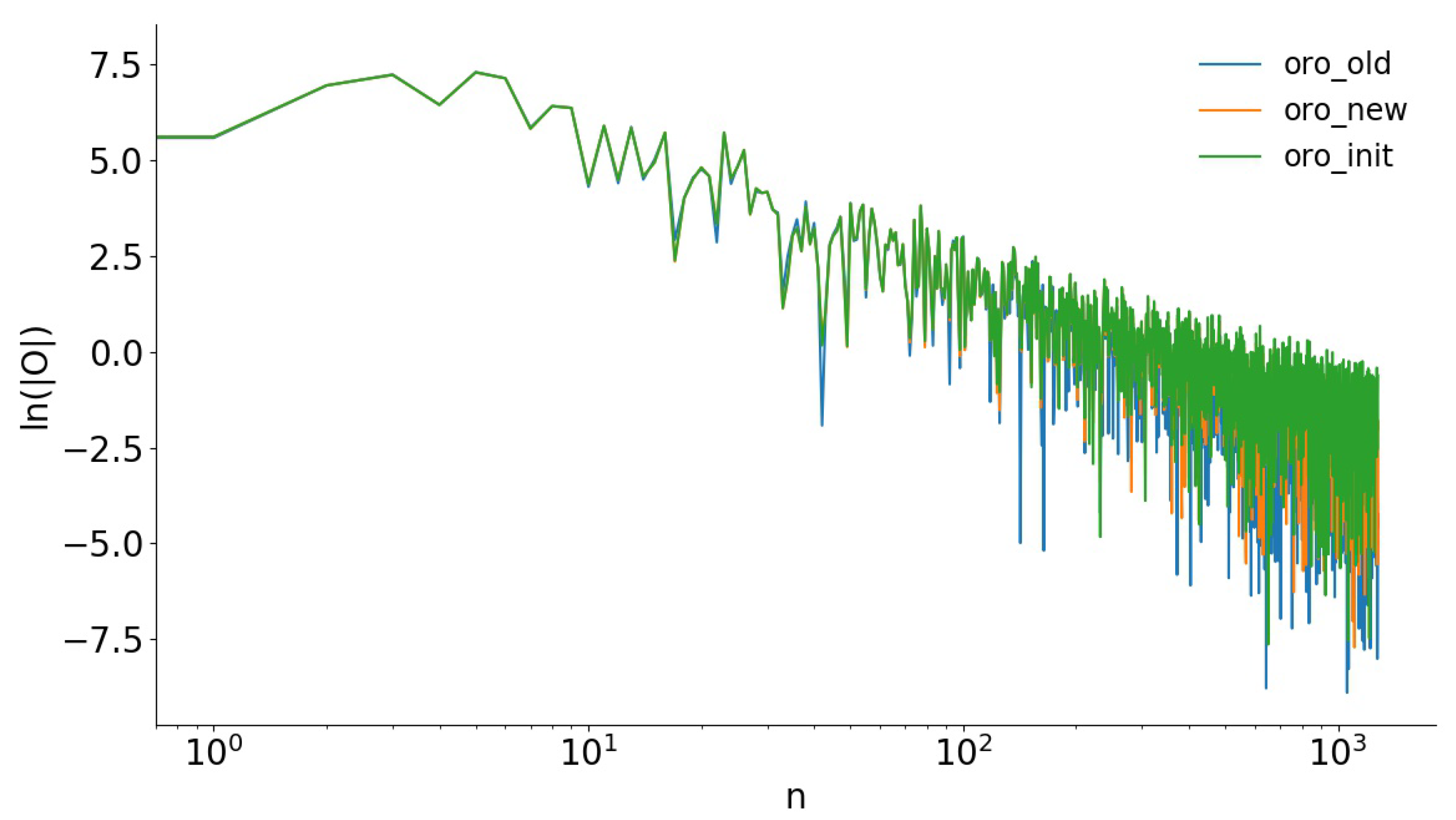
2.3. Processing Steps for Orographic Data

(1)

The first filtering is performed on the initial global orographic dataset with a resolution of 30′′. The filter scale $\gamma$ is set to 5 km, and the edge scale $\delta$ is set to 1 km. The filter scale $\gamma$ is set according to the requirements of the scale information to be filtered out. The edge scale $\delta$ affects the overall filtering effect. Therefore, it should not be set too large, generally to 1 km. The purpose of this step is to filter out the orographic features below the 5 km scale because, as described in Section 1, orographic features below the 5 km scale should be described in the TOFD parameterization scheme. These small-scale orographic information in the dynamics of patterns will not be conducive to NWP. It would be detrimental to NWP if these small-scale orographic features are retained in the model’s dynamics.

(2)

After the filtering operation in the first step, the orographic dataset is interpolated to a resolution of 2′30′′ (the grid spacing near the equator is about 5 km). The purpose of this step is mainly to prepare for the second filtering and to separate the different orographic scale information.

(3)

The second filtering is carried out on the orographic dataset with a resolution of 2′30′′. The filter scale $\gamma$ is set to 16 km, and the edge scale $\delta$ is set to 1 km. The purpose of this step is to filter out orographic features below 16 km because the resolution of YHGSM used in this study is T1279 (the grid spacing around the equator is about 16 km). Orographic features from 5 km to grid spacing (about 16 km) should be described in Sub-grid Scale Orography (SSO) parameterization schemes to optimize orographic effects in NWP models. When performing two-dimensional filtering in this step, the weights in Equation (3) need to be adjusted slightly to $G_3=0$, $P_3=0$, and $G_2=0.362$ due to the change in the grid distance.

(4)

After the filtering operation in the second step, the orographic dataset is interpolated from a 2′30′′ resolution to a 7′30′′ resolution (the grid spacing near the equator is about 16 km). The purpose of this step is mainly to prepare for the next second filtering and to separate the different orographic scale information. The purpose of this step is to get closer to the model’s resolution before performing the spectral transformation. However, the interpolation operation reduces the resolution of the orographic dataset, which means that some small-scale orographic features are lost. To discuss whether keeping higher resolution before spectral transformation is more beneficial to NWP, a switch is set in this step.

(5)

The grid orographic dataset is converted to spectral orography with a target resolution of T1279. Numerical weather prediction spectral models generally choose a spherical harmonic as the basis function. The spherical harmonic is as follows:

$$Y_n^m\left(\lambda , \mu \right)=e^{im\lambda }{P}_n^m\left(\mu \right)$$

(4)

where $\lambda$ is latitude, $\upsilon =\sin \phi$, $\phi$ is longitude, and $P_n^m\left(\mu \right)$ is the associated Legendre polynomial. The relation between the orographic height $O\left(\lambda , \mu \right)$ in the grid space and the spectral coefficient $O_n^m$ is as follows:

$$O\left(\lambda , \upsilon \right)={{\displaystyle \sum }}_{m-\infty }^{\infty }{{\displaystyle \sum }}_{n=\left|m\right|}^{\infty }{O}_n^m{Y}_n^m\left(\lambda , \upsilon \right)={{\displaystyle \sum }}_{m-\infty }^{\infty }{{\displaystyle \sum }}_{n=\left|m\right|}^{\infty }{O}_n^m{e}^{im\lambda }{P}_n^m\left(\mu \right).$$

(5)

The above transformation process is mainly divided into two steps. The first step is the Fourier transform (Equation (6)), and the second step is the Legendre transform (Equation (7)):

$$C^m\left(\mu \right)=\frac{1}{2\pi }{{\displaystyle \int }}_0^{2\pi }O\left(\lambda , \mu \right)e^{-im\lambda }d\lambda ,$$

(6)

$$O_n^m={{\displaystyle \int }}_{-1}^1{C}^m\left(\mu \right)P_n^m\left(\mu \right)d\mu$$

(7)

where $C^m\left(\mu \right)$ is the Fourier coefficient. Numerous spectral coefficients are involved in the above calculations. As m and n increase, the scale of the orography described by the spectral coefficients becomes finer. However, in practical numerical calculations, we can only consider a limited number of spectral coefficients, i.e., wavenumber truncation. The resolution of the NWP spectral model is determined by the maximum truncation number of m and n, where m is the zonal wave number, and n is the total wave number. The maximum zonal wave number is 1279, and the maximum value of n is obtained using the triangular truncation method.

The orographic spectral coefficients $O_n^m=a_n^m+i{b}_n^m$ obtained using Equation (7) need to be filtered in spectral space. $O_n^m$ is multiplied by $f\left(n\right)$ in Equation (8) to avoid spectral aliasing.

$$f\left(n\right)=\frac{1}{1+4\times {\left(\frac{n}{mmax}\times \frac{n+1}{mmax}\right)}^8}$$

(8)

where $mmax=1279$ is the maximum truncated wave number. The number of spectral coefficients is determined by the maximum truncated wave number $mmax$:

$$number of spectral coefficients=\left(mmax+1\right)\times \left(mmax+2\right)/2.$$

(9)

The first ten thousand components of the orographic spectral coefficient are taken for analysis. In order to see the difference more intuitively, we used logarithmic coordinates for analysis. These orographic spectral coefficients, $O_n^m=a_n^m+i{b}_n^m$, are transformed using Equation (10).

$$ln\left(\left|O\right|\right)=ln(\sqrt{a^2+b^2)}$$

(10)

Thus, the natural logarithm of the first 1000 orographic spectral coefficients is obtained (Figure 3). The global large-scale orographic characteristics of the new orography obtained through the above process, the orography without the above processing, and the model’s original orography, especially for the first 10 spectral components, are basically the same. After the first 100 spectral components, there are some obvious differences among the three orography. It can be seen that the above orography processing operations do not change the large-scale features of the orography, and they only change the small-scale details of the orography.

At present, there is no research on whether keeping a higher resolution grid-point field before transferring it to the spectral space is beneficial to improving the performance of the model. Therefore, when designing experiments, a switch was set for the operation of step (4) in the processing steps of the orographic data to conduct comparative experiments and explore whether maintaining a higher orographic resolution before transforming it to spectral space is beneficial to the model’s ability to simulate the extreme rainfall event in Henan. Five groups of experiments were conducted (

Table 1. Experiment settings.

Experiment Name	With or Without Step (4)	Grid-Point Filter
Exp 1	Yes	bidirectional one-dimensional filter
Exp 2	No	bidirectional one-dimensional filter
Exp 3	Yes	direct two-dimensional filter
Exp 4	No	direct two-dimensional filter
Exp 0	Model’s old orography

). Exp0 was the control experiment, in which the model’s original orography was used. Wang et al. [36] used the same configuration as exp0 when studying the effect of orographic resolution on NWP model simulations. They found that the YHGSM performed best using the orography of exp0. In this study, the experimental results of exp0 were used as benchmarks. Exp1–exp2 were the comparative experiments, using the orography processed using the two different filters. In both, the YHGSM was used to simulate the extreme rainfall in Henan on 19 and 20 July 2021 to explore the impact of using the different types of filters on the orography and the maintenance of a higher orographic resolution before transferring it to the spectral space for the simulation of extreme weather events. All of the measured rainfall data used in this study were obtained from the China Meteorological Administration, and all of the rainfall classification levels are defined according to the classification of rainfall grades in inland China developed by the China Meteorological Administration (

Table 2. Classification standards of the rainfall intensity in the inland areas of China.

Rainfall Level	24 h Total Rainfall (mm)
Light rainfall	0.1–9.9
Moderate rainfall	10.0–24.9
Heavy rainfall	25.0–49.9
Torrential rainfall	50.0–99.9
Big torrential rainfall	100.0–249.9
Extraordinarily torrential rainfall	≥250.0

).

3. Results

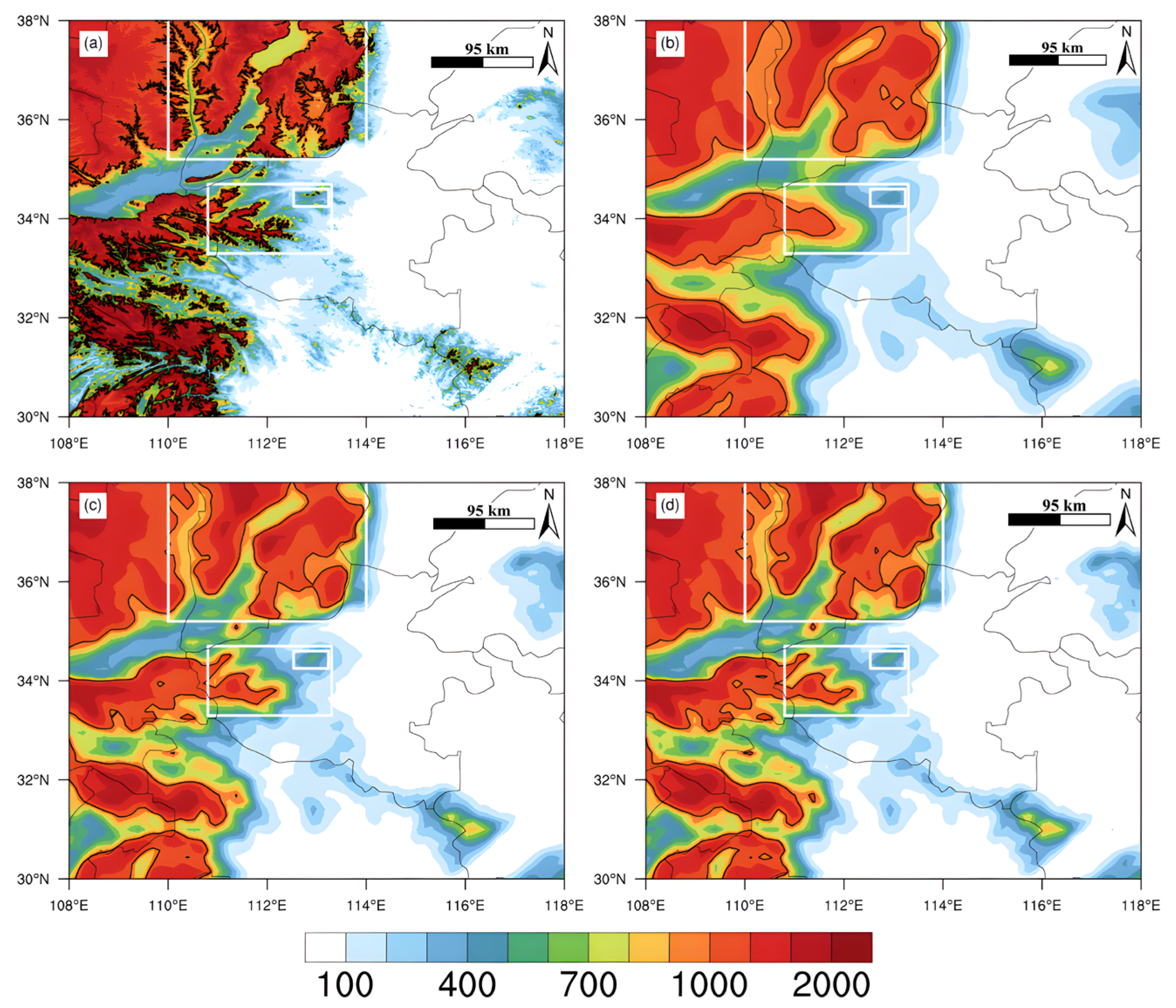
3.1. Overview of the Study Area

Henan Province is located in the central part of eastern Asia and the orographic features high in the west and low in the east (Figure 4). Henan is located at the junction between the western mountains and eastern plains. The Taihang Mountains are located on the northwest side of Henan, with an average altitude of over 1200 m. The Funiu Mountains are located on the west side, with an altitude of over 1000 m. The main part of the Funiu Mountains is located on the western edge of Henan. Among them, Songshan is located near the center of Henan, and its highest peak exceeds 1000 m. The Loess Plateau and Qinghai-Tibet Plateau are located to the west of the Taihang and Funiu mountains. This orographic feature causes warm and moist airflow from the South China Sea and the Western Pacific to converge or climb when it is blocked by the mountains, providing a good backdrop for rainfall. It can be seen from Figure 4 that the new unprocessed orography retains many small-scale detail features, while the model’s original orography is relatively smooth and can only describe some of the larger-scale features. By comparing Figure 4c,d, it was found that the bidirectional one-dimensional filter filtered out more of the small-scale, detailed orographic features than the direct two-dimensional filter. The direct two-dimensional filter preserved some of the high peaks in western Henan.

The main precipitation area was set as the zone (32–36°N, 110–116°E). There are 145 meteorological observation stations in the main precipitation area. Among them, Zhengzhou Station had an hourly rainfall of 201.9 mm at around 9:00 on 20 July 2021, setting a record in China and causing great damage to the environment and people [36]. Figure 5 shows hourly changes in total rainfall in the main precipitation area. Before the peak rainfall period, the total hourly rainfall on the 19th was mostly less than 400 mm. The total hourly rainfall on the 20th was mostly greater than 400 mm, and the maximum value could reach 656.5 mm. It can be clearly seen that the rainfall intensity on the 19th was much weaker than that on the 20th.

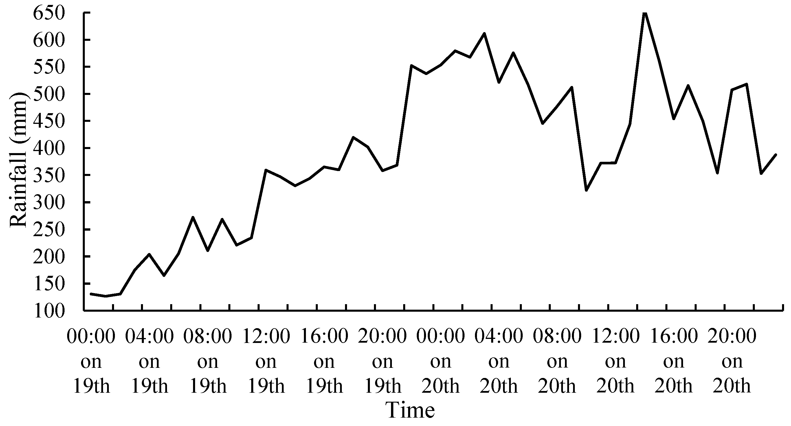
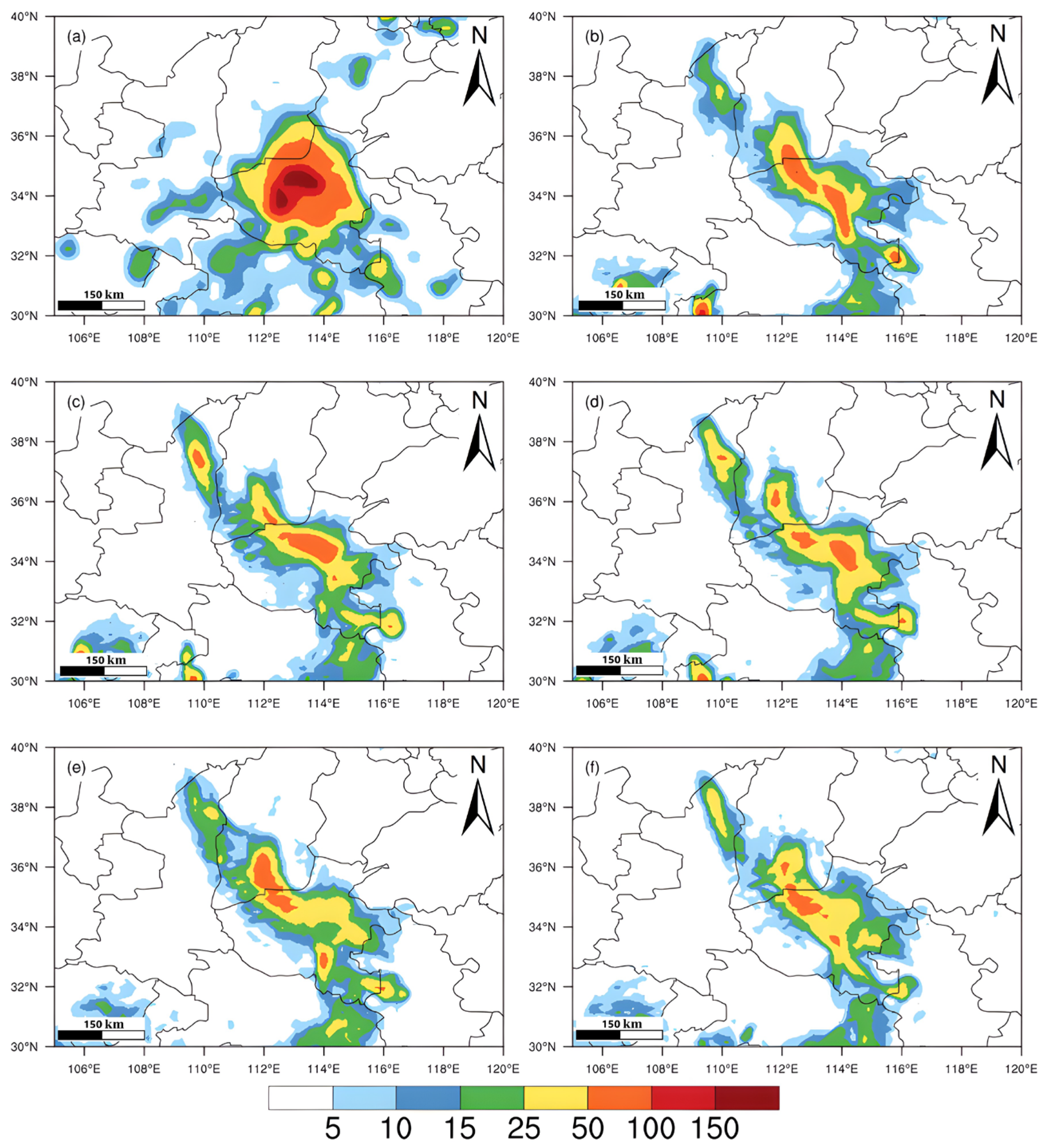
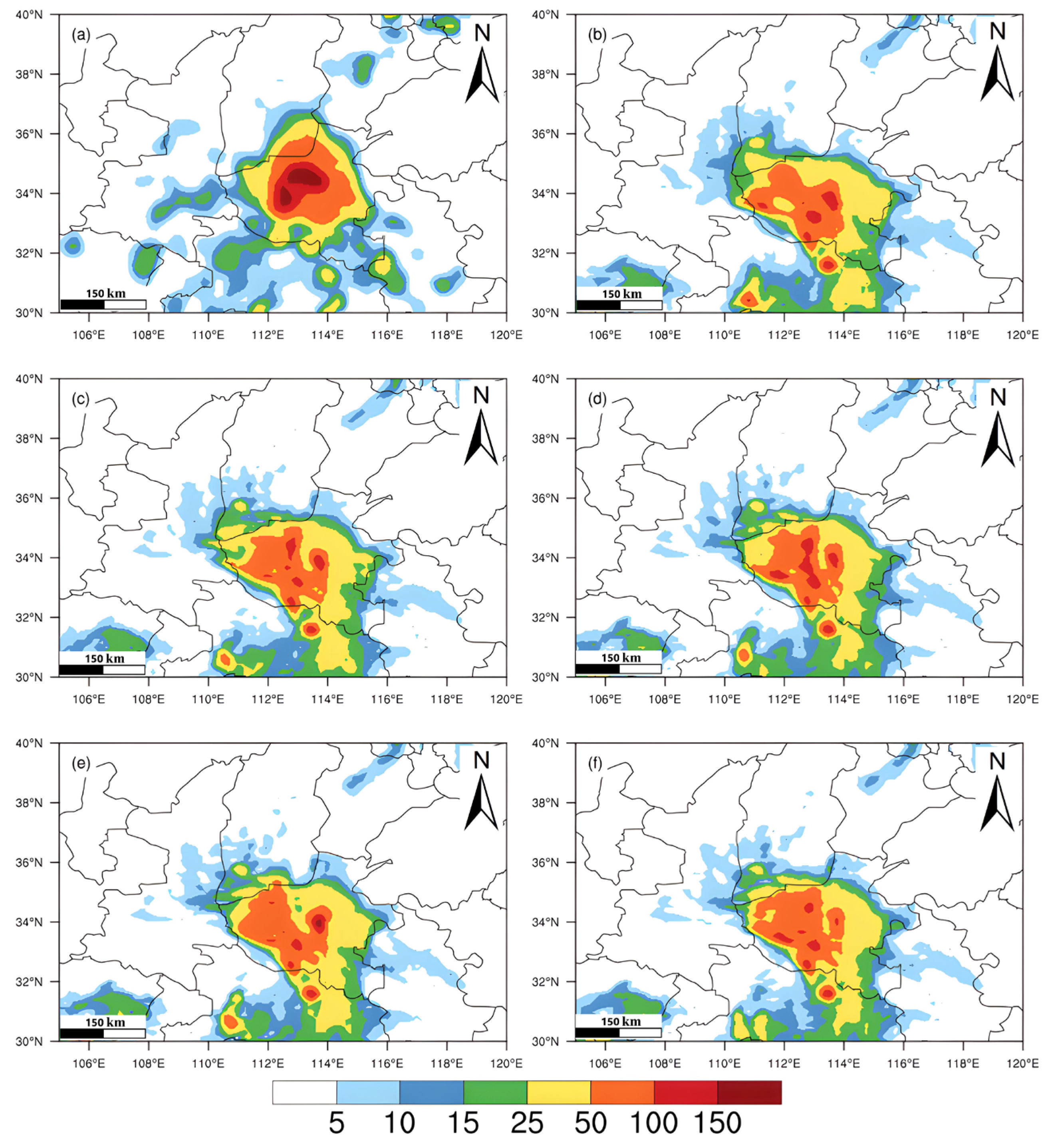
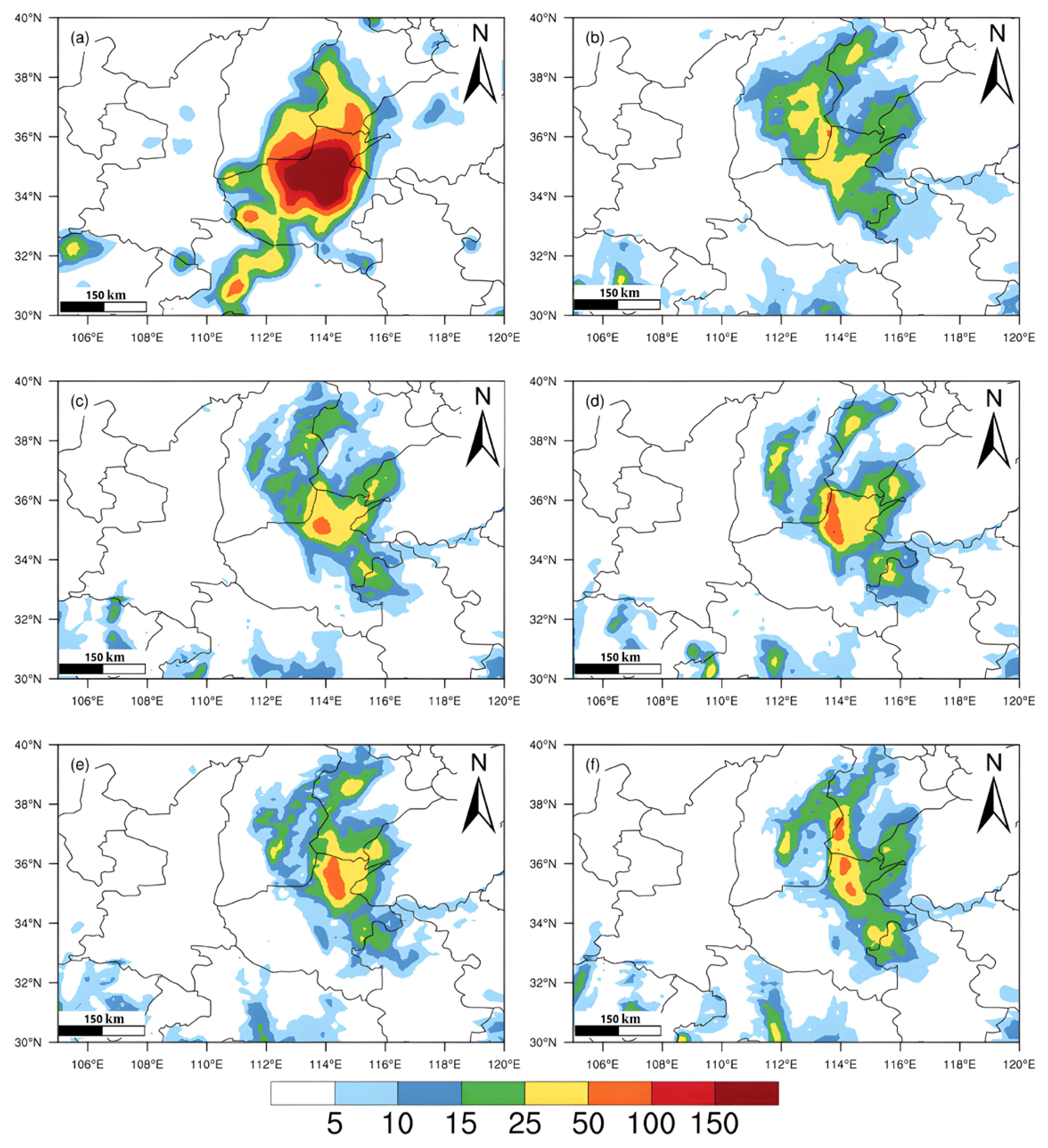
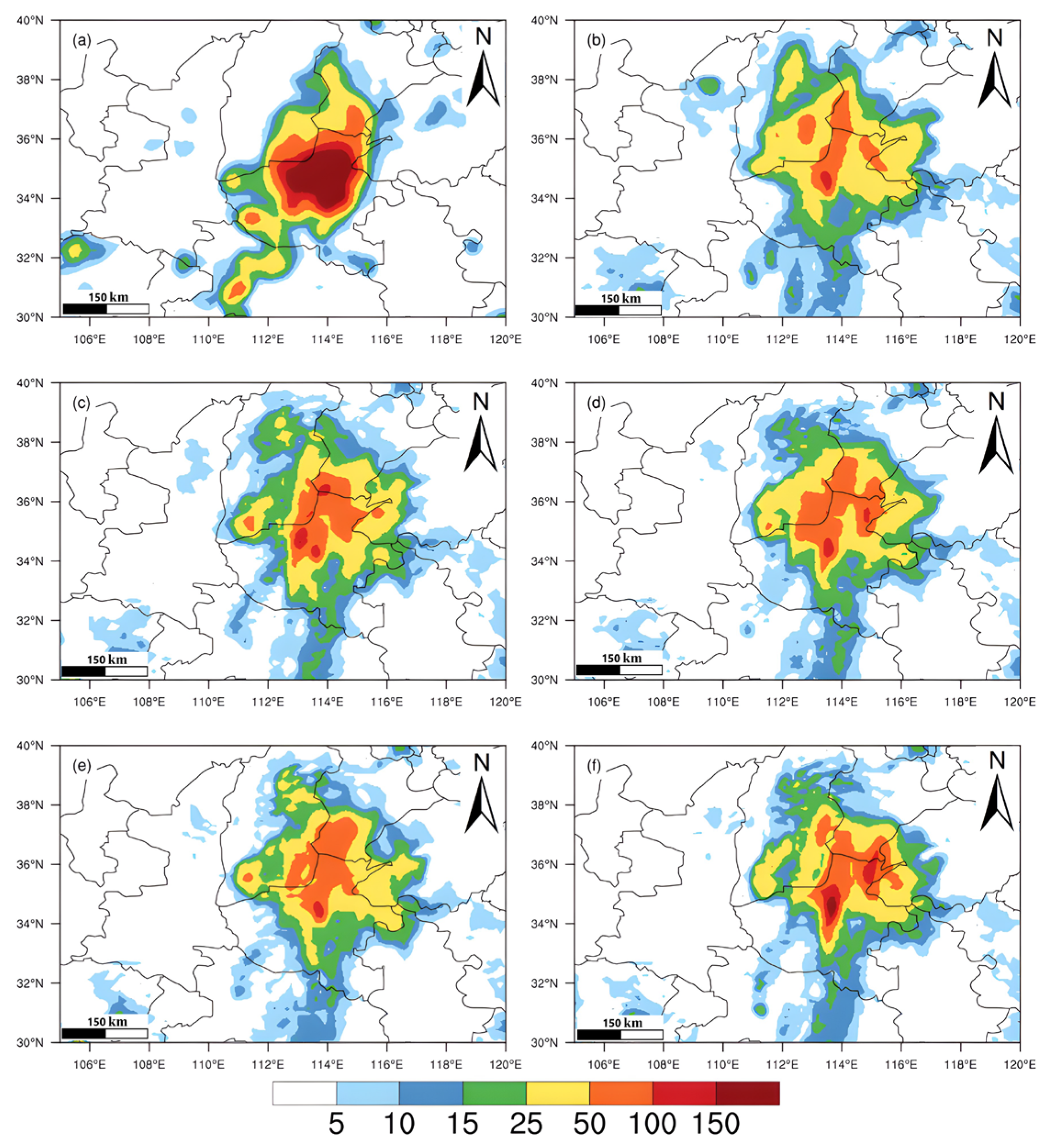
3.2. Simulation of Extreme Rainfall in Henan

In order to understand the influence of starting the model at different times on the extreme rainfall simulation results obtained, we ran the model at 00:00 on the 18th and 00:00 on the 19th, and then we compared and analyzed the 24 h accumulated rainfall from 00:00 to 23:00 on the 19th and that from 00:00 to 23:00 on the 20th (Figure 6, Figure 7, Figure 8 and Figure 9). Figure 6a was obtained by interpolating the actual rainfall values observed at the meteorological stations onto a two-dimensional plane. According to the classification of rainfall levels in inland China developed by the China Meteorological Administration (Table 2), the rainfall range was at least heavy-rainfall level over most of Henan on the 19th, and the area in which the rainfall range was above the torrential-rainfall level was mainly distributed in the central and northwestern parts of Henan. When the model was started at 00:00 on the 18th, the simulated rainfall range and rainfall intensity of the 24 h cumulative rainfall on the 19th was smaller than the actual rainfall, but it also reflected the main rainfall areas, which were mainly distributed in the central and northwestern regions of Henan. Both exp1 (Figure 6c) and exp2 (Figure 6d), which were conducted using the bidirectional one-dimensional filter, simulated the rainfall level near Zhengzhou well. Compared with exp1, the distribution of the precipitation above the torrential-rainfall level in exp2 was scattered, and the range was smaller. The torrential-rainfall level precipitation simulated by both exp3 (Figure 6e) and exp4 (Figure 6f), which was conducted using the direct two-dimensional filter, was shifted to the northwest in Henan. In exp3, the torrential-rainfall area was shifted to the southern part of Shanxi Province, creating a false torrential-rainfall area. The torrential-rainfall area simulated in exp4 was smaller than that produced in exp3. It can be seen that the simulations for exp3 and exp4 were obviously worse than those for exp1 and exp2. Two torrential-rainfall centers were obtained in exp0 (Figure 6b) using the model’s original orography. Compared with exp0, the torrential-rainfall level areas simulated in exp1 were more concentrated, and there was almost no false torrential-rainfall area.

Figure 6 and Figure 7 have significant differences in terms of the rainfall area and rainfall intensity, indicating that starting the model at different times has a great influence on the simulation results. In the simulations of the model started at 00:00 on the 19th, the heavy-rainfall level basically covered all of Henan on the 19th, which was similar to the measured heavy-rainfall level area. The rainfall range and rainfall intensity were obviously larger and stronger than the simulation results of the model started at 00:00 on the 18th. In exp1 (Figure 7c) and exp2 (Figure 7d) (bidirectional one-dimensional filter), the range of the torrential-rainfall level extended farther north. The big-torrential-rainfall level had more areas in exp2 than in exp1. In exp3 (Figure 7e) and exp4 (Figure 7f) (direct two-dimensional filter), the area of the big-torrential-rainfall level was smaller. An extraordinarily-torrential-rainfall level area was simulated in exp3, but its range was far smaller than the measured range. In exp0 (Figure 7b) (model’s original orography), the torrential-rainfall was mainly distributed in the southwestern part of Henan, while the measured torrential-rainfall level areas were mainly distributed in the central part of Henan. The rainfall areas above the big-torrential level simulated in exp1–exp4 were significantly larger than that for exp0, especially that of exp2, which was more similar to the measured rainfall.

The 24 h accumulated rainfall from 00:00 to 23:00 on 20 July for the model started at 00:00 on 18 July 2021 is shown in Figure 8. It can be seen that the model simulation was not very good, and a possible reason for this is that the model’s start time was too late. In exp1 (Figure 8c) and exp2 (Figure 8d) (bidirectional one-dimensional filter), the torrential-rainfall level was simulated, but the rainfall area was small. The torrential-rainfall area in exp2 was larger than that in exp1. In exp3 (Figure 8e) and exp4 (Figure 8f) (direct two-dimensional filter), the model also simulated the torrential-rainfall level. In exp4, part of the torrential-rainfall area moved northward into Hebei, resulting in false torrential-rainfall areas. In exp0 (Figure 8b) (model’s original orography), the torrential-rainfall level area was hardly simulated. It can be seen that even when the model simulations are poor, using new orography can slightly improve the simulation results.

The 24 h cumulative rainfall from 00:00 to 23:00 on 20 July for a model start time of 00:00 on 19 July 2021 is shown in Figure 9. It can be seen that the simulation was significantly improved. This confirms the above conclusion; that is, the simulation results of the model started at 00:00 on the 19th were better than the simulation results of the model started at 00:00 on the 18th. As can be seen from the simulation results of the model started at 00:00 on the 19th (Figure 9), the heavy-rainfall level basically covered the area of the measured heavy-rainfall distribution. In exp0 (Figure 9b) (model’s original orography), some false heavy-rainfall level regions were simulated in Shanxi and Shandong, and the simulated torrential-rainfall level area was smaller than the measured torrential-rainfall area. The simulation results of exp1 (Figure 9c) and exp2 (Figure 9d) (bidirectional one-dimensional filter) produced larger torrential-rainfall areas, and both simulations were better than that of exp0. The big-torrential-rainfall level areas in exp1 were larger than those in exp2. In exp3 (Figure 9e) and exp4 (Figure 9f) (direct two-dimensional filter), the main rainfall center shifted northward. Exp3 produced a small false torrential-rainfall level area in the southern part of Hebei Province. In exp4, the area of the heavy-rainfall level was reduced, but it simulated the extraordinarily-torrential-rainfall level, which was located near Zhengzhou. In general, for the simulations of the rainfall on 20 July 2021, the simulations conducted in exp1–exp4 using the new orography were better than the simulation conducted in exp0 using the model’s original orography. In most cases, the simulations conducted using the bidirectional one-dimensional filter were better than the simulations conducted using the direct two-dimensional filter. However, in a few cases, much larger rainfall levels were simulated when using a direct two-dimensional filter.

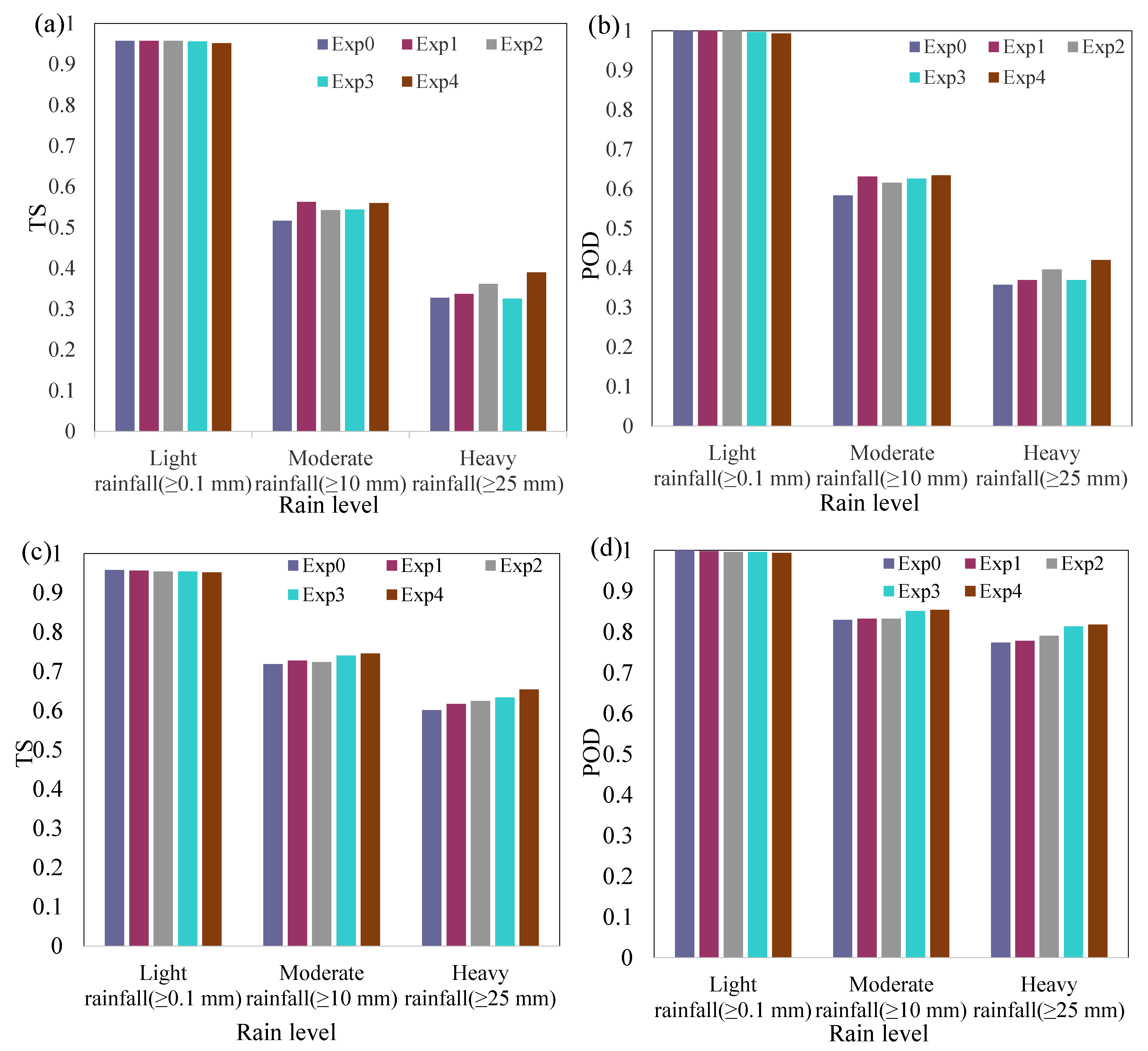
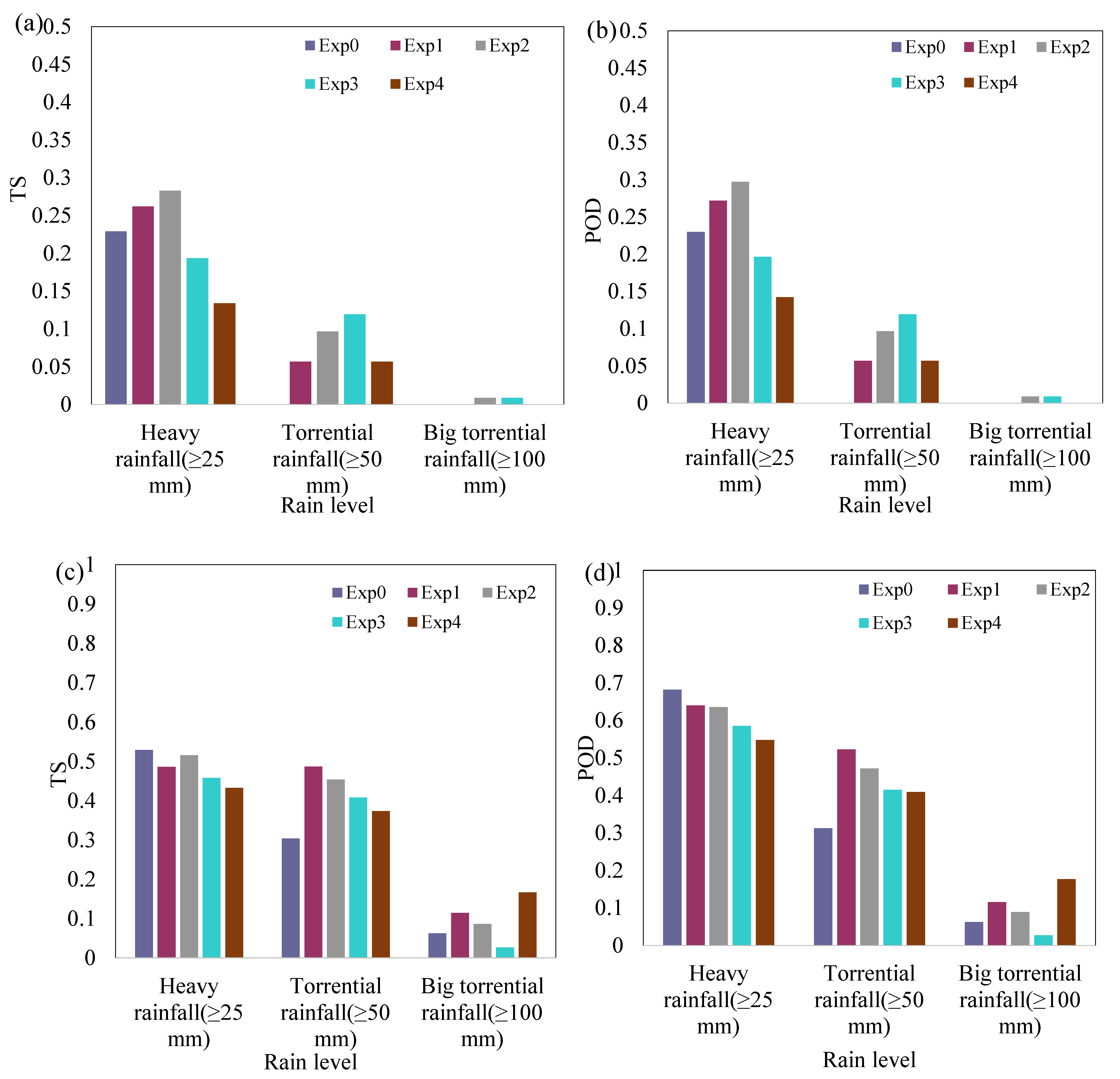
3.3. Quantitative Analysis of Rainfall Simulations

When predicting rainfall, a threshold $\alpha$ is usually used to distinguish between the rainfall levels and/or whether rainfall occurs. In order to more clearly evaluate the improvement of the Henan 20·7 extreme rainfall simulation using the new orography, we used two evaluation indicators, the threat score ($TS$), and the probability of detection ($POD$), which are defined as follows:

$$TS=\frac{Hits}{Hits+False alarms+Misses},$$

(11)

$$POD=\frac{Hits}{Hits+Misses}$$

(12)

$Hits$ represents the number of grid points in which the actual rainfall exceeds the threshold $\alpha$ in the area where the predicted rainfall exceeds the threshold $\alpha$; $Misses$ represents the number of grid points that are predicted not to exceed the threshold $\alpha$ in the area where the measured rainfall exceeds the threshold $\alpha$; and $False alarms$ represents the number of grid points where the actual rainfall does not exceed the threshold $\alpha$ in the area where the predicted rainfall exceeds the threshold $\alpha$. The $TS$ is a comprehensive index used to evaluate the quality of the rainfall simulation. The $POD$ index is the proportion of the actual rainfall area simulated by the model compared to the total actual rainfall area.

The measured rainfall data from 145 meteorological observation stations in the main precipitation area (32–36°N, 110–116°E) in Henan were used to calculate the evaluation indexes. The Cressman interpolation method was used to interpolate the measured station data to the same resolution as the model’s forecast data to evaluate the $TS$ and $POD$ indexes, as shown in Figure 10 and Figure 11. It can be seen from the results presented in Section 3.2 that the rainfall intensity on 19 July was obviously weaker than that on 20 July. Therefore, for the 24 h cumulative rainfall in Henan on 19 July, the $TS$ and $POD$ indexes of the heavy-rainfall level and below were mainly analyzed and evaluated (Figure 10). For the 24 h cumulative rainfall in Henan on 20 July, the $TS$ and $POD$ indexes of the heavy-rainfall level and above were mainly analyzed and evaluated (Figure 11). As can be seen from Figure 10, the simulations conducted using the newly orography significantly improved both the moderate-rainfall level and heavy-rainfall level. According to the simulations obtained using the model started at 00:00 on 18 July (Figure 10a,b), the $TS$ and $POD$ indexes of the light-rainfall in each experiment are similar and are close to 1. For both the moderate-rainfall level and the torrential-rainfall level, the simulations conducted using the new orography are superior to the simulations conducted using model’s original orography. For the moderate-rainfall level, the differences in the $TS$ and $POD$ values of exp1–exp4 are not significant. For the heavy-rainfall level, the $TS$ and $POD$ values of exp2 and exp4 (the orography maintains a higher resolution before conversion into the spectral space) are significantly higher than those of exp1 and exp3 (the orography is interpolated before converting it into the spectral space). From the results of the model started at 00:00 on 19 July (Figure 10c,d), it can be seen that both the $TS$ and $POD$ are higher than those of the results for the model started at 00:00 on 18 July. This demonstrates that the simulation error of the model started closer to the time of the extreme rainfall is smaller and the rainfall evaluation score is higher.

For the rainfall on 20 July, the heavy-rainfall level and above were mainly analyzed and evaluated (Figure 11). It can also be seen from Figure 11 that the simulations of Henan on 20 July obtained using the new orography are also significantly improved in terms of the heavy-rainfall level and above. According to the results of the model started at 00:00 on 18 July (Figure 11a,b), the $TS$ and $POD$ values of exp3 and exp4 (direct two-dimensional filter) for the heavy-rainfall level are lower than those of exp0 (model’s original orography). The $TS$ and $POD$ values of exp1 and exp2 (bidirectional one-dimensional filter) are higher than those of exp0, which is consistent with the results of the analysis of the rainfall distribution in Section 3.2. In terms of the torrential-rainfall level and big-torrential-rainfall level, exp0 (model’s original orography) does not simulate the torrential-rainfall and big-torrential-rainfall in the main areas of Henan, and its $TS$ and $POD$ values are equal to or close to 0 (Figure 8b). However, exp1–exp4 (new orography) simulate the torrential-rainfall level with different degrees of accuracy, and their $TS$ and $POD$ values are greatly improved compared with those of exp0. In addition, $TS$ and $POD$ values of exp2 and exp3 are both greater than 0 for the big-torrential-rainfall level. This demonstrates that the model that uses the new orography improves the simulations of the Henan 20·7 extreme rainfall event and can successfully simulate the torrential-rainfall level and big-torrential-rainfall level.

According to the results of the model started at 00:00 on the 19th (Figure 11c,d), the $TS$ and $POD$ values of exp0–exp4 are greatly improved compared with those of the model started at 00:00 on 18 July (Figure 11a,b). For the heavy-rainfall level, the $TS$ and $POD$ values of exp1–exp4 (new orography) are slightly lower than those of exp0 (model’s original orography). A possible reason for this is that exp0 simulated many false heavy-rainfall areas outside of Henan (Figure 9). However, the calculation of $TS$ in this study mainly considers the rainfall in Henan Province, resulting in the false heavy-rainfall areas failing to affect the $TS$ value. Therefore, the $TS$ value in exp0 may be lower than the current value if the larger rainfall range is considered when calculating the $TS$. For the torrential-rainfall level, the $TS$ and $POD$ values of exp1–exp4 (new orography) are higher than those of exp0 (model’s original orography). The $TS$ and $POD$ values of exp1 and exp2 (bidirectional one-dimensional filter) are higher than those of exp3 and exp4 (direct two-dimensional filter). For the big-torrential-rainfall level, the $TS$ and $POD$ values of exp1–exp4 are also higher than those of exp0, which once again confirms that, regarding the simulation of the Henan 20·7 extreme rainfall event, the results of this model can be improved by using the new orography. The $TS$ value of exp4 is about three times that of exp0, and the simulation of the big-torrential-rainfall level is significantly improved.

3.4. Analysis of Heavy Rain in Beijing

Beijing is located in the northern part of Henan Province (about 39–41°N, 115–117°E). It also experienced strong precipitation on 16 and 17 July 2021. The precipitation at a single station can reach a maximum of more than 226 mm. In order to more effectively verify the validity and superiority of the newly constructed orography, this paper also analyzes the heavy rainfall in Beijing on 16 and 17 July. The maximum width from east to west is about 160 km, and the maximum width from north to south is about 176 km in Beijing. It is very challenging for a global NWP model to predict or simulate a weather event in the small area of Beijing. It can be seen that using the YHGSM is a little difficult to improve the simulation of this heavy rainfall event in Beijing. Based on the analysis in Section 3.2 and Section 3.3, the bidirectional one-dimensional filter is used to filter orography of Beijing and its surrounding, as shown in Figure 12. The Beijing is located at the intersection of plains and mountains, with the Yanshan Mountains to the north and the Taihang Mountains to the west. The Beijing’s orographic features is high in the west and low in the east, high in the north and low in the south. In the unfiltered orography (Figure 12a), there are many peaks over 1000 m in the northwest of Beijing. After the filtering operation (Figure 12b), these peaks above 1000 m were almost filtered out. In the model’s original orography, the orographic height is smoother, and some small-scale orographic features are no longer visible.

The rainfall intensity in Beijing on July 16 was less than that on July 17 (Figure 13a,b). Except for heavy-rainfall in a small area, the overall rainfall in Beijing on July 16 was moderate-rainfall. It can be seen from Figure 13a that there are three rainfall centers from north to south, the ranges of the three rainfall centers were relatively small, and the rainfall center in the north had the highest intensity. From simulation results of the model using the original orography (Figure 13e), it can be seen that the central and southern rainfall centers were not successfully simulated, and the northern rainfall range was too large, resulting in large false rainbands. From the simulation results of the model using the new orography (Figure 13b), it can be seen that the false rainband in the north disappeared, and the rainfall range was reasonably controlled. Two small rainfall centers in northern and central Beijing were connected. Although the southern rainfall center was not successfully simulated, the overall effect of the simulation was better than the simulation results using the model’s original orography. The rainfall intensity in Beijing on 17 July was relatively high, with two big-torrential-rainfall centers (Figure 13b). The YHGSM simulation results were generally small, and these two small-scale heavy rain areas have not been successfully simulated. However, when using the model’s original orography, YHGSM failed to simulate both rainfall centers, only a small area of moderate-rainfall, and also deviated from the actual rainfall center. When using the new orography, YHGSM was able to successfully simulate two heavy-rainfall centers. Although the rainfall intensity was lower than the actual rainfall, the location of the rainfall centers was similar to the location of the actual rainfall centers. In conclusion, although it is difficult for a global model to accurately simulate the weather in this small-scale area of Beijing, YHGSM’s simulation of heavy rain in Beijing has been significantly improved after using the new orography produced.

4. Discussion

In this study, based on ASTER GDEM V3 data, global orographic datasets were produced using different orographic processing operations. The YHGSM was used to simulate the early and peak periods of the Henan 7·20 extreme rainfall event. The results of the simulations conducted using the new global orographic datasets were compared with the results of the simulations conducted using the model’s original orography to verify the new orography. Finally, in order to more effectively verify the effectiveness and superiority of the new orography, YHGSM also used the new orography to simulate the heavy rain in Beijing from 16 to 17 July 2021.

The main difference between the bidirectional one-dimensional filter and the direct two-dimensional filter is that the bidirectional one-dimensional filter maintains a uniform filter scale globally, while the direct two-dimensional filter maintains a uniform number of filter grid-points globally. Due to this characteristic and fact that the Earth is approximately spherical, the bidirectional one-dimensional filter has more grid-points near the poles and fewer near the equator, while the direct two-dimensional filter has a smaller filter scale near the poles and a larger filter scale near the equator. Therefore, they have similar filter scales near the equator. In the nonequatorial regions, the direct two-dimensional filter has a smaller filter scale, which may preserve some of the small-scale orographic features. Based on Figure 3, it was also found that these processing operations only changed the small-scale orographic features, but they all produced similar global large-scale orographic features. From the orographic map of Henan, it was found that the processing of the orography filtered out many of the small-scale orographic features. The bidirectional one-dimensional filter made the orography smoother than the direct two-dimensional filter, and the model’s original orography was the smoothest.

Whether it was the simulation of light-rainfall, moderate-rainfall, and heavy-rainfall on 19 July in Henan or the simulation of the torrential-rainfall and big-torrential-rainfall on 20 July, we found that with the increase in rainfall level, the $TS$ and $POD$ values gradually decreased. This indicates that the model’s simulation bias increases as the rainfall level increases, which is consistent with the findings of Hu et al. [37]. It can be seen that there is an extremely urgent need to improve the simulation performance of extreme rainfall events above the torrential-rainfall level.

Based on the simulations of the extreme rainfall event in Henan on 19 July, the simulations conducted using the bidirectional one-dimensional filter were better than the simulations conducted using the direct two-dimensional filter. However, for the simulations conducted using the direct two-dimensional filter, it was sometimes found that larger levels of rainfall were simulated. A possible reason for this is that the direct two-dimensional filter retained higher mountain heights in the western orography of Henan, which further blocked the movement of the airflow, causing the warm and humid airflow to converge here and cause greater rainfall. For the heavy-rainfall level, maintaining a higher orographic resolution before transferring it to the spectral space may lead to the simulation of more heavy-rainfall areas. This is probably because the mountain height was not further smoothed by the interpolation, resulting in the Gibbs phenomenon mentioned earlier [17]. The increased valleys and mountains of the Gibbs phenomenon can cause the convergence and climb of airflows, which can cause precipitation. Lindberg’s integrated studies at a range of horizontal resolutions of the Geophysical Fluid Dynamics Laboratory (GFDL) climate model also showed that Gibbs ripples can lead to small-scale extremes in the spatial distribution of precipitation [19].

For the simulations of the extreme rainfall event in Henan on 20 July, when the model started at 00:00 on 18 July, the model’s original orography failed to simulate the torrential-rainfall level area. The simulations were improved by using the new orography, and small areas of torrential-rainfall level were simulated. For the simulations when the model started at 00:00 on 19 July, the simulations conducted using the bidirectional one-dimensional filter were better than those conducted using the direct two-dimensional filter in most cases. In a few cases, the model obtained larger rainfall levels when using the direct two-dimensional filter, as shown in the 19 July simulation results. This may be because the model uses orography that has been processed by a direct two-dimensional filter to produce a stronger orographic effect. For the heavy-rainfall level, the simulation conducted using the model’s original orography had a higher $TS$ value. Based on Figure 9, a possible reason for this is that many simulated false heavy rainfall areas outside Henan failed to affect the $TS$ value because of the calculation range of $TS$. The $TS$ value in the simulations using the model’s original orography may be lower than the current value if the larger rainfall range is considered when calculating the $TS$. In conclusion, in most cases, the simulations conducted using the new orography were better than the simulations conducted using the model’s original orography. This paper optimized the orographic description in YHGSM dynamics. Orographic effects are actually described in both the dynamics and physical process parameterization of the NWP model, and the two parts are interrelated. Therefore, the next research plan may be needed to optimize the description of the orographic effect in the parameterization scheme when the filter removes the small-scale orographic features that cannot be described by the NWP model dynamics, so that the orographic effect in the parameterization scheme is approximately equal to that which cannot be described by model dynamics.

5. Conclusions

This study developed a set of orographic construction techniques for NWP spectral models. In orographic processing, both the bidirectional one-dimensional filter and the direct two-dimensional filter are successful against many small-scale orography, but they retain greater orographic realism without over-smoothing compared to the model’s original orography. The bidirectional one-dimensional filter has a larger filtering degree, and the direct two-dimensional filter has a weaker filtering degree, retaining some small-scale orographic features. The new orography constructed based on the ASTER GDEM dataset significantly improves the simulations of the Henan 20·7 extreme rainfall event and the heavy rain in Beijing.

In general, for the simulations of the Henan 20·7 extreme rainfall event, the bidirectional one-dimensional filter was found to be superior to the direct two-dimensional filter in terms of the orographic processing. The bidirectional one-dimensional filter can filter out more of the small-scale orographic information that is harmful to the model prediction, and the direct two-dimensional filter can sometimes simulate more intense rainfall. The effect of maintaining the higher orographic resolution before conversion to the spectral space is not very significant, but it was found that it can lead to the simulation of more heavy-rainfall level areas. In conclusion, in most cases, the YHGSM using the new global orographic dataset based on ASTER GDEM data outperformed that using the model’s original orographic dataset, especially regarding simulation of the torrential-rainfall level and above.

References

1. IPCC. AR6 Climate Change 2021: The Physical Science Basis; IPCC: Geneva, Switzerland, 2021. [Google Scholar] [CrossRef]
2. Xia, Z.; Hui, Y.; Xinmin, W.; Lin, S.; Di, W.; Han, L. Analysis on characteristic and abnormality of atmospheric circulations of the July 2021 extreme precipitation in Henan. Trans. Atmos. Sci. 2021, 44, 672–687. [Google Scholar] [CrossRef]
3. Wenru, S.; Xin, L.; Mingjian, Z.; Bing, Z.; Hongbin, W.; Kefeng, Z.; Xiaoyong, Z. Multi-model comparison and high-resolution regional model forecast analysis for the “7·20” Zhengzhou Severe Heavy Rain. Trans. Atmos. Sci. 2021, 44, 688–702. [Google Scholar] [CrossRef]
4. Sandu, I.; Niekerk, A.V.; Shepherd, T.G.; Vosper, S.B.; Svensson, G. Impacts of orography on large-scale atmospheric circulation. Clim. Atmos. Sci. 2019, 2, 10. [Google Scholar] [CrossRef]
5. Berckmans, J.; Woollings, T.; Demory, M.-E.; Vidale, P.-L.; Roberts, M. Atmospheric blocking in a high resolution climate model: Influences of mean state, orography and eddy forcing. Atmos. Sci. Lett. 2013, 14, 34–40. [Google Scholar] [CrossRef]
6. Wang, Y.; Wu, J. Overview of the Application of Orographic Data in Numerical Weather Prediction in Complex Orographic Areas. Adv. Meteorol. 2022, 2022, 1279625. [Google Scholar] [CrossRef]
7. Chenghai, W.; Xiao, L.; Yi, Y. Atmospheric Numerical Model and Simulation; China Meteorological Press: Beijing, China, 2011; pp. 109–110. [Google Scholar]
8. Berkofsky, L.; Bertoni, E.A. Mean Topographic Charts for the Entire Earth. Bull. Am. Meteorol. Soc. 1955, 36, 350–354. [Google Scholar]
9. Nikolakopoulos, K.G. Comparing a DTM created with ASTER data to GTOPO 30 and to one created from 1/50.000 topographic maps. Proc. SPIE 2004, 5574, 43–51. [Google Scholar]
10. Nikolakopoulos, K.G.; Kamaratakis, E.K.; Chrysoulakis, N. SRTM vs ASTER elevation products. Comparison for two regions in Crete, Greece. Int. J. Remote Sens. 2006, 27, 4819–4838. [Google Scholar] [CrossRef]
11. Farr, T.G.; Rosen, P.A.; Caro, E.; Crippen, R.; Duren, R.; Hensley, S.; Kobrick, M.; Paller, M.; Rodriguez, E.; Roth, L.; et al. The Shuttle Radar Topography Mission. Rev. Geophys. 2007, 45, 1–33. [Google Scholar] [CrossRef] [Green Version]
12. Danielson, J.J.; Gesch, D.B. Global Multi-Resolution Terrain Elevation Data 2010 (GMTED2010); U.S. Geological Survey: Reston, VA, USA, 2011.
13. Husain, S.Z.; Separovic, L.; Girard, C. On the Need of Orography Filtering in a Semi-Lagrangian Atmospheric Model with a Terrain-Following Vertical Coordinate. In Proceedings of the 19th Conference on Mountain Meteorology, Dorval, QC, Canada, 15 July 2020. [Google Scholar]
14. Vosper, S.B.; Brown, A.R.; Webster, S. Orographic drag on islands in the NWP mountain grey zone. Q. J. R. Meteorol. Soc. 2016, 142, 3128–3137. [Google Scholar] [CrossRef]
15. Davies, L.A.; Brown, A.R. Assessment of which scales of orography can be credibly resolved in a numerical model. Q. J. R. Meteorol. Soc. 2001, 127, 1225–1237. [Google Scholar] [CrossRef]
16. Gassmann, A. Filtering of LM-orography. COSMO Newsl. 2000, 1, 71–78. [Google Scholar]
17. Florinsky, I.V. Chapter 5—Errors and Accuracy. In Digital Terrain Analysis in Soil Science and Geology (Second Edition); Florinsky, I.V., Ed.; Academic Press: Cambridge, MA, USA, 2016; pp. 149–187. [Google Scholar]
18. Veregin, H. The Effects of Vertical Error in Digital Elevation Models on the Determination of Flow-path Direction. Cartogr. Geogr. Inf. Syst. 1997, 24, 67–79. [Google Scholar] [CrossRef]
19. Lindberg, C.; Broccoli, A.J. Representation of Topography in Spectral Climate Models and Its Effect on Simulated Precipitation. J. Clim. 1996, 9, 2641–2659. [Google Scholar] [CrossRef]
20. Bouteloup, Y. Improvement of the Spectral Representation of the Earth Topography with a Variational Method. Mon. Weather. Rev. 1995, 123, 1560–1574. [Google Scholar] [CrossRef] [Green Version]
21. Navarra, A.; Stern, W.F.; Miyakoda, K. Reduction of the Gibbs Oscillation in Spectral Model Simulations. J. Clim. 1994, 7, 1169–1183. [Google Scholar] [CrossRef] [Green Version]
22. Raymond, W.H.; Garder, A. A Spatial Filter for Use in Finite Area Calculations. Mon. Weather. Rev. 1988, 116, 209–222. [Google Scholar] [CrossRef] [Green Version]
23. Webster, S.; Brown, A.R.; Cameron, D.R.; Jones, C.P. Improvements to the representation of orography in the Met Office Unified Model. Q. J. R. Meteorol. Soc. 2003, 129, 1989–2010. [Google Scholar] [CrossRef]
24. Raymond, W.H. High-Order Low-Pass Implicit Tangent Filters for Use in Finite Area Calculations. Mon. Weather. Rev. 1988, 116, 2132–2141. [Google Scholar] [CrossRef]
25. Rutt, I.; Thuburn, J.; Staniforth, A. A variational method for orographic filtering in NWP and climate models. Q. J. R. Meteorol. Soc. 2007, 132, 1795–1813. [Google Scholar] [CrossRef]
26. Guanghui, W.; Fengfeng, C.; Xueshun, S.; Jianglin, H. The impact of topography filter processing and horizontal diffusion on precipitation prediction in numerical model. Chin. J. Geophys. 2008, 51, 1642–1650. [Google Scholar]
27. Abrams, M.; Crippen, R.; Fujisada, H. ASTER Global Digital Elevation Model (GDEM) and ASTER Global Water Body Dataset (ASTWBD). Remote Sens. 2020, 12, 1156. [Google Scholar] [CrossRef] [Green Version]
28. Tachikawa, T.; Kaku, M.; Iwasaki, A.; Gesch, D.; Oimoen, M.; Zhang, Z.; Danielson, J.; Krieger, T.; Curtis, B.; Haase, J. ASTER Global Digital Elevation Model Version 2—Summary of Validation Results; NASA: Washington, DC, USA, 2011. [Google Scholar]
29. Peng, J.; Wu, J.; Zhang, W.; Zhao, J.; Zhang, L.; Yang, J. A modified nonhydrostatic moist global spectral dynamical core using a dry-mass vertical coordinate. Q. J. R. Meteorol. Soc. 2019, 145, 2477–2490. [Google Scholar] [CrossRef]
30. Yin, F.; Wu, G.; Wu, J.; Zhao, J.; Song, J. Performance Evaluation of the Fast Spherical Harmonic Transform Algorithm in the Yin–He Global Spectral Model. Mon. Weather. Rev. 2018, 146, 3163–3182. [Google Scholar] [CrossRef]
31. Jiang, T.; Guo, P.; Wu, J. One-sided on-demand communication technology for the semi-Lagrange scheme in the YHGSM. Concurr. Comput. Pract. Exp. 2020, 32, e5586. [Google Scholar] [CrossRef]
32. Peng, J.; Zhao, J.; Zhang, W.; Zhang, L.; Wu, J.; Yang, X. Towards a dry-mass conserving hydrostatic global spectral dynamical core in a general moist atmosphere. Q. J. R. Meteorol. Soc. 2020, 146, 3206–3224. [Google Scholar] [CrossRef]
33. Yang, J.; Song, J.; Wu, J.; Ying, F.; Peng, J.; Leng, H. A semi-implicit deep-atmosphere spectral dynamical kernel using a hydrostatic-pressure coordinate. Q. J. R. Meteorol. Soc. 2017, 143, 2703–2713. [Google Scholar] [CrossRef]
34. Yang, J.; Song, J.; Wu, J.; Ren, K.; Leng, H. A high-order vertical discretization method for a semi-implicit mass-based non-hydrostatic kernel. Q. J. R. Meteorol. Soc. 2015, 141, 2880–2885. [Google Scholar] [CrossRef]
35. Jianping, W.; Jun, Z.; Junqiang, S.; Weiming, Z. Preliminary design of dynamic framework for global non-hydrostatic spectral mode. Comput. Eng. Des. 2011, 32, 3539–3543. [Google Scholar] [CrossRef]
36. Wang, Y.; Wu, J.; Peng, J.; Yang, X.; Liu, D. Extreme Rainfall Simulations with Changing Resolution of Orography Based on the Yin-He Global Spectrum Model: A Case Study of the Zhengzhou 20·7 Extreme Rainfall Event. Atmosphere 2022, 13, 600. [Google Scholar] [CrossRef]
37. Hu, Y.-F.; Yin, F.-K.; Zhang, W.-M. Deep learning-based precipitation bias correction approach for Yin–He global spectral model. Meteorol. Appl. 2021, 28, e2032. [Google Scholar] [CrossRef]
Figure 1. Curve of a one-dimensional Gaussian distribution function.
Remotesensing 14 03840 g001
Figure 2. Distribution of two-dimensional grid. The darkest squares have Manhattan distance ≤ 1, the lightest squares have Manhattan distance = 3, and the squares in between have Manhattan distance = 2.
Remotesensing 14 03840 g002
Figure 3. Natural logarithm of the moduli of the first 1000 orographic spectral coefficients. Model’s original orography (oro_old), orography after processing (oro_new), and the initial orography before processing (oro_init).
Remotesensing 14 03840 g003
Figure 4. Orographic height (unit: m): (a) the new initial orography before processing, (b) the model’s original orography, (c) new orography processed using the bidirectional one-dimensional filter, and (d) new orography processed using the direct two-dimensional filter. The solid black lines are the 1000 m contour lines. The two large white rectangles represent Taihang Mountains (top) and Funiu Mountains (bottom). The small white rectangle in the lower rectangle represents Songshan mountain, which is part of Funiu Mountain.
Remotesensing 14 03840 g004
Figure 5. Hourly changes in total rainfall measured in the main precipitation area from 00:00 on 19 July to 23:00 on 20 July 2021.
Remotesensing 14 03840 g005
Figure 6. The 24 h cumulative rainfall (unit: mm) from 00:00 to 23:00 on 19 July with a model start time of 00:00 on the 18th: (a) measured rainfall, (b) exp0, (c) exp1, (d) exp2, (e) exp3, and (f) exp4.
Remotesensing 14 03840 g006
Figure 7. The 24 h cumulative rainfall (unit: mm) from 00:00 to 23:00 on July 19 with a model start time of 00:00 on the 19th: (a) measured rainfall, (b) exp0, (c) exp1, (d) exp2, (e) exp3, and (f) exp4.
Remotesensing 14 03840 g007
Figure 8. The 24 h cumulative rainfall (unit: mm) from 00:00 to 23:00 on 20 July with a model start time of 00:00 on the 18th: (a) measured rainfall, (b) exp0, (c) exp1, (d) exp2, (e) exp3, and (f) exp4.
Remotesensing 14 03840 g008
Figure 9. The 24 h cumulative rainfall (unit: mm) from 00:00 to 23:00 on 20 July with a model start time of 00:00 on the 19th: (a) measured rainfall, (b) exp0, (c) exp1, (d) exp2, (e) exp3, and (f) exp4.
Remotesensing 14 03840 g009
Figure 10. Evaluation indexes of the 24 h cumulative rainfall from 00:00 to 23:00 on 19 July. (a,b) are the results of the model started at 00:00 on 18 July, (c,d) are the results of the model started at 00:00 on 19 July, (a,c) show the T S values, (b,d) show the P O D values.
Remotesensing 14 03840 g010
Figure 11. Evaluation indexes of the 24 h cumulative rainfall from 00:00 to 23:00 on 20 July. (a,b) are the results of the model started at 00:00 on 18 July, (c,d) are the results of the model started at 00:00 on 19 July, (a,c) show the TS values, (b,d) show the POD values.
Remotesensing 14 03840 g011
Figure 12. Orographic height (unit: m): (a) the new initial orography before processing, (b) new orography processed using the bidirectional one-dimensional filter, and (c) the model’s original orography.
Remotesensing 14 03840 g012
Figure 13. The 24 h cumulative rainfall (unit: mm) on 16 and 17 July 2021 with the model start time of 00:00 on the 15th: (a,c,e) are the rainfall on 16 July, (b,d,f) are the rainfall on 17 July. (a,b) Measured rainfall, (c,d) rainfall simulated using the new orography, (e,f) rainfall simulated using the model’s original orography.
Remotesensing 14 03840 g013