Article

Evolution and Structure of a Dry Microburst Line Observed by Multiple Remote Sensors in a Plateau Airport

1
Plateau Atmosphere and Environment Key Laboratory of Sichuan Province, School of Atmospheric Sciences, Chengdu University of Information Technology, Chengdu 610225, China
2
Meteorological Observatory, Qinghai Sub-Bureau, Civil Aviation Administration of China Northwest Region Air Traffic Management Bureau, Xining 810000, China
3
State Key Laboratory of Severe Weather, Chinese Academy of Meteorological Science, Beijing 100081, China
4
Quanzhou Jinjiang International Airport, Quanzhou 362299, China
*
Author to whom correspondence should be addressed.
Remote Sens. 2022, 14(15), 3841; https://doi.org/10.3390/rs14153841
Submission received: 16 June 2022 / Revised: 27 July 2022 / Accepted: 5 August 2022 / Published: 8 August 2022
(This article belongs to the Special Issue Synergetic Remote Sensing of Clouds and Precipitation)

Abstract

:
The civilian airplane is a common transportation mode for the local people in the Qinghai-Tibet Plateau (QTP). Due to the profound dynamic and thermal effects, the QTP can trigger strong windstorms during the warm season, during which downbursts can cause severe low-level wind shear and threaten aviation safety. However, the study of downbursts over QTP has not been given much attention. This study analyzes and interprets a typical traveling dry microburst line that happened at the Xining Caojiapu International Airport (ZLXN) on 14 May 2020, intending to show a better understanding of the dry downbursts over QTP and explore the synergetic usage of different remote sensing technologies for downburst detection and warning in plateau airports. Specifically, the characteristics of synoptic conditions, the convective system formation process, and the structure and evolution of downbursts and relevant low-level winds are comprehensively investigated. The results show that, under the control of an upstream shallow trough, features of the local atmosphere state, including a dry-adiabatic stratification, a shallow temperature inversion, increases in solar radiation heating, and strong vertical shears of horizontal winds, can be favorable atmospheric prerequisites for the formation and development of dry storms and downbursts. Low-reflectivity storm cells of the Mesoscale Convective System (MCS) organize to form narrow bow echoes, and downbursts show features of radial wind convergences and rapid descending reflectivity cores with hanging virga as observed by a Doppler weather radar. Moreover, details of gales, gust fronts, convergences, turbulences, wind collisions, and outflow interactions triggered by the downburst line are also detected and interpreted by a scanning Doppler wind lidar from different perspectives. In addition, the findings in this work have been compared with the results observed in Denver, U.S., and some simulation studies. Finally, a few conceptual models of low-level wind evolutions influenced by the dry downburst line are given.

1. Introduction

Downbursts are small-scale intense outflows produced by storms or strong cumulonimbuses [1,2], which can cause damaging gales and wind shear. In general, a downburst can be grouped into macroburst and microburst based on its outflow dimension. A macroburst is larger than a microburst with a horizontal extent of more than 4 km in diameter [3,4]. However, a microburst can develop into a macroburst after expanding in space under favorable atmospheric circumstances [5]. According to accompanied rain amount ( R a , mm), downbursts also can be subdivided into dry ( R a ≤ 0.25 mm) and wet ( R a > 0.25 mm) types [1,6,7]. Although the driving mechanisms of these different downbursts are unique, their destructive capabilities threaten human life and property, making comprehensive observations and studies of them of significant importance and necessity.
In the aviation community, microbursts constitute a significant threat to flight safety that has been reported by many previous investigations [6,8,9]. This hazardous meteorological phenomenon attracted public attention for the first time after Flight 66 of Eastern Airlines crashed while attempting to land in New York on 24 June 1975 [10]. As it is closely related to aircraft accidents and incidents, many field experiments, including Northern Illinois Meteorological Research on Downburst Project (NIMROD, 1978) [10], Joint Airport Wind Shear Project (JAWS, 1982) [11], FAA-Lincoln Laboratory Operational Weather Studies (FLOWS, 1985) [12], and Microburst and Severe Thunderstorm Project (MIST, 1986) [13], were conducted during the late 1970s and 1980s in the U.S. Specifically, NIMROD aimed to validate the existence of downburst wind events. JAWS was conducted in Denver, Colorado, to primarily explore environmental conditions for microburst formation and study their outflow structure and evolution on the high plains. In FLOWS, an automatic weather station network was built to locate and reveal the surface wind characteristics of microbursts and to confirm the wind shear detected by Doppler weather radars. The MIST project is an experiment conducted near Huntsville, Alabama, to study downbursts in a relatively humid environment. Based on these experiments, more sophisticated and profound explanations of the microbursts’ formation and evolution mechanisms were proposed. Caracena and Flueck (1987) [11] pointed out that a dry downburst can be typically triggered by a strong evaporative cooling effect when hydrometeors rapidly fall into the dry atmosphere. They also confirmed that microburst events seem predictable, and simple forecasting schemes can be driven using the local radiosonde data. Several favorable indicators for forecasting dry downbursts in Denver, U.S., were summarized as: the existence of a surface shallow radiation inversion in the forenoon, a deep dry-adiabatic layer, appropriate sub-cloud mixing ratios, and enough convection temperatures [12]. Hjelmfelt (1988, 1987) [13,14] found that complicated outflows can be more often caused by a microburst line, which simultaneously consists of multiple downbursts with their outflows forming an outward divergence line. Compared to a single microburst, such linear downbursts commonly possess longer life cycles and larger footprints and also lead to stronger winds and more significant impacts. Following Hjelmfelt et al.’s observational findings, some subsequent research focused on simulating the near-surface wind fields and outflow interactions. Orf (1996) [15] and Vermeire (2011) [16] suggested that the downburst line can form in three distinct patterns, including coalescing, complex interacting, and Soliton-like noninteracting. The wind damage caused by the downburst line during its coalescing and complex interacting periods can be several times stronger than that of the individual downburst event.
Several recent studies [17,18,19,20] have affirmed the experiments and relevant studies on the downburst mentioned above in the U.S. Nevertheless, those studies provide little real-time information on the fine structure of wind fields caused by the downburst’s outflow collision. Moreover, those findings still have limited geographical applicability. For instance, to the best of our knowledge, no one has used meteorological and field campaign data to investigate or warn about dry microburst lines yet in the Qinghai-Tibet Plateau (QTP) of China, a region that possesses frequent convection activity [21], though the civil airplane has been the main mode of transportation for the local people. Therefore, for aviation safety, more observations and studies are needed to better understand the characteristics and environmental conditions of downbursts in such a particular area.
In general, Doppler Weather Radar (DWR) and ground Automated Weather Observing System (AWOS) have been common equipment for monitoring and warning about upcoming thunderstorms and relevant damaging winds around an airport of interest. However, these two observational technologies have shortcomings in precisely observing the low-reflectivity dry microbursts and their wind fields. The DWR can only detect the reflected echoes of liquid or ice hydrometeors under rainy conditions [22], and the AWOS is strictly bound to ground observation. Laser-based instruments, such as Doppler Wind Lidar (DWL), can be an alternative candidate. The scanning DWL can detect high-spatiotemporal-resolution wind fields under non-rainy conditions, which provides a desirable way for investigating the fine structure and evolution details of downbursts and relevant winds [23,24].
This study is motivated by an aircrew report: “go around (GA), which can reset an effective opportunity to stack the odds back in the favor of a pilot to safely land an aircraft in hazardous conditions” when an airplane tried landing at Xining Caojiapu International Airport (located in the northeast of the QTP) under the influence of a dry downburst line event on 14 May 2020. First, we attempt to exploit the synergetic usage of DWR, airport AWOS, and DWL for observation and warning about the dry downburst line. Additionally, measurements from multiple sensors were comprehensively analyzed to reveal the variation, structure, and evolution of dry microbursts in this high-altitude airport. The following contents are organized as: Section 2 describes the geographical background of the airport as well as the instruments used and their measurements. Section 3 briefly introduces data processing methods for the DWR. Detailed analysis and results regarding synoptic conditions and variations, structures, and evolutions of mesoscale convection and relevant microbursts are presented in Section 4. Section 5 gives a comparison and discussion between our findings and counterparts from other areas, and previous simulation works are also further confirmed. In Section 6, we end with a summary of our conclusions.

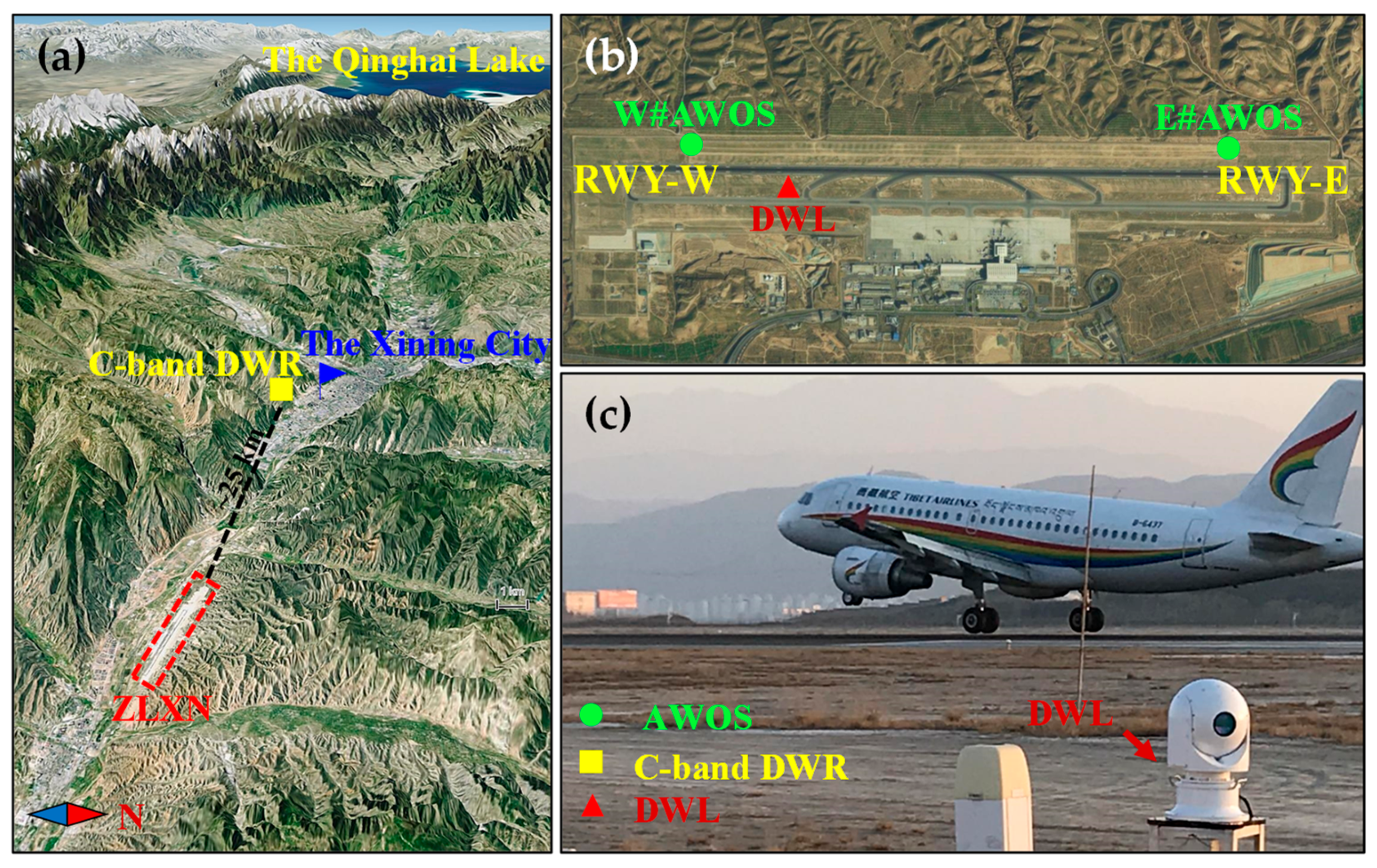
2. Airport, Instruments, and Measurements

The Xining Caojiapu International Airport (denoted by the International Civil Aviation Organization code of ZLXN hereafter) is an important transportation hub for the Qinghai Province and Tibet Autonomous Region of China. It is a 4E-class civil plateau airport located in the northeast of the QTP at an altitude of 2184 m. As shown in Figure 1, the airport is located in a valley approximately 28 km away from the Xining city center. It possesses a southeast-to-northwest oriented runway with a length of 3800 m and magnetic directions of 110° and 290°. For convenience, two sides of the runway are marked as RWY-W and RWY-E as shown in Figure 1b, which denotes the west and east sides of the runway, respectively. Due to complex terrain, irregular winds, and low-level airflow disturbances can frequently affect the airport. The unique topography also results in inhomogeneous flows when convections affect the area, making outflow behaviors and evolutions more unpredictable.
Three types of meteorological remote sensors, including a C-band DWR, a scanning DWL, and two sets of AWOS, were employed in this study. Their installed positions are shown in Figure 1. Detailed information about these sensors and measurements are briefly depicted as follows:
(1)
C-band DWR. It is a member of the China Next Generation Weather Radar (CINRAD) network and was deployed approximately 25 km northwest of ZLXN. The radar takes six minutes to perform a routine VCP-21 (Volume Coverage Pattern) scan that contains nine elevation layers (i.e., 0.5°, 1.5°, 2.4°, 3.4°, 4.3°, 6.0°, 9.9°, 14.6°, and 19.5°). It can provide observations with an effective detection radius of 150 km and a range gate spacing of 300 m. Due to the extensive detection range, radar volume-scanning data are utilized to provide a view of horizontal and vertical organizations of reflectivity and radial velocity, and then infer the cloud-precipitation structure and evolution as well as prominent features of the convective system;
(2)
DWL. In recent years, with a rapid increase in the flight volume of ZLXN, aircraft pilot reports on low-level wind shear and turbulence under non-rainy conditions are also increasing. Therefore, to fill in a gap for wind detection in fair-weather conditions, a scanning DWL manufactured by the No.209 Institute of China North Industries Group Corporation Limited was installed near the runway in 2017. The DWL is a coherent-pulsed lidar operating with a wavelength of 1.55 µm and a pulse repetition frequency of 10 kHz. The laser energy and pulse width of the DWL are 100 µJ per pulse and 355/500/667 ns (adjustable), respectively. The DWL’s effective detection radius is 8–10 km, and the spatial resolution is available at 50/75/100 m. A combined scanning strategy was implemented to achieve three-dimensional detection of wind fields and provide alarms on low-level wind shear. It includes one Doppler-beam-swinging (DBS) scan, four plan-position-indicator (PPI) scans, two glide-path (GP) scans, and two range-height-indicator (RHI) scans. The DBS provides zenithal profiles of vertical and horizontal winds, while the PPI obtains omnidirectional radial velocity, spectrum width, and retrieved wind fields in elevations of 3° and 6° (corresponding to plane angles of aircraft landing and take-off). The GP anticipates observing the headwind and crosswind of the glide path, and the RHI gives cross-sections of radial winds along the runway direction. The combined scanning strategy performs in a sequence of “DBS–PPI(3°)–GP–PPI(4°)–GP–PPI(3°)–RHI–PPI(3°)–RHI” and its whole process takes ~15 min. The main specifications of the DWL are listed in Table 1;
(3)
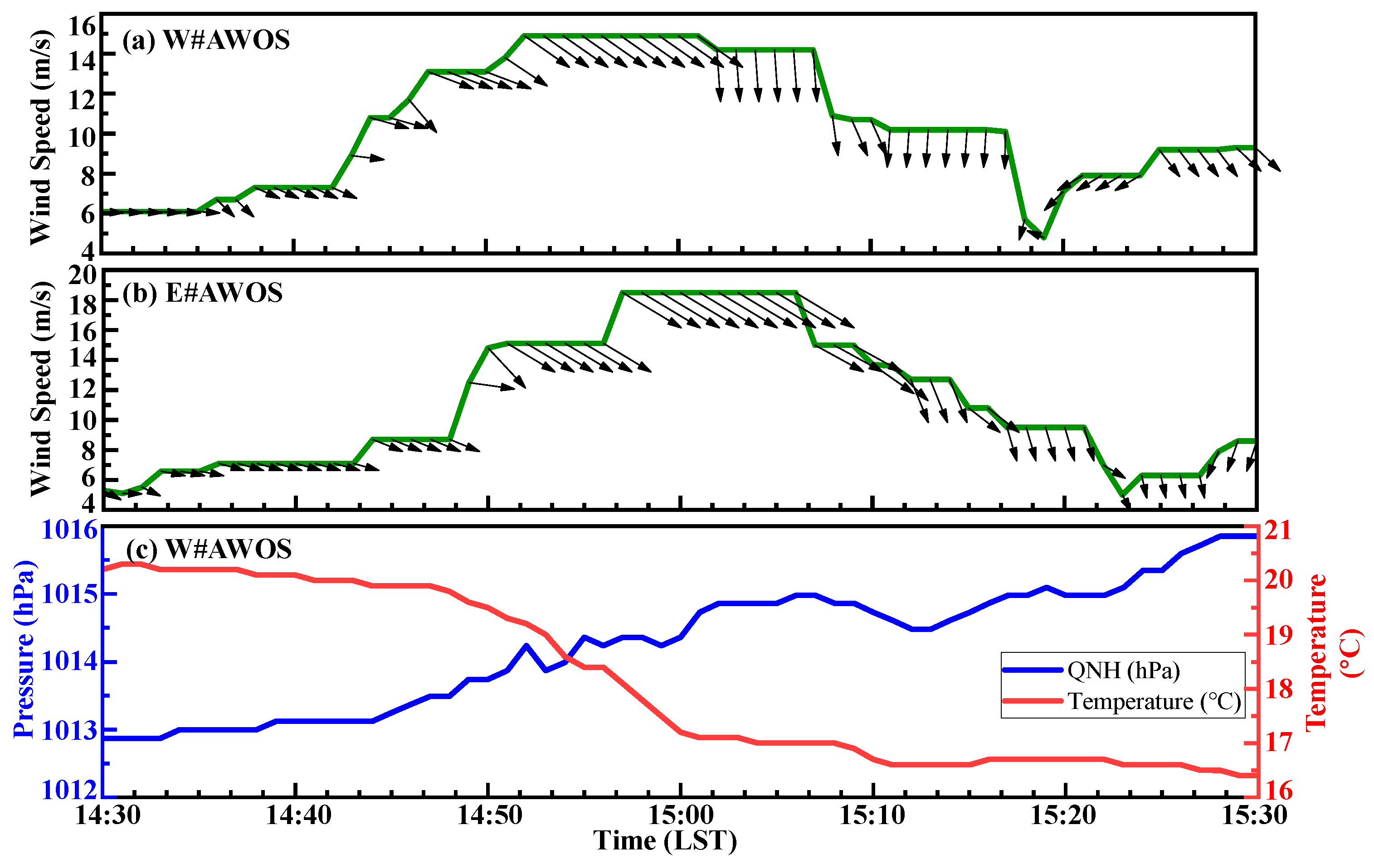
AWOS. As a resident instrument deployed in the civil aviation airport, the AWOS is a set of ground meteorological sensors and information transmission systems manufactured according to the technical standards of the International Civil Aviation Organization and the World Meteorological Organization (WMO). It is usually installed near the airport runway to provide continuous and real-time meteorological data for air traffic controllers and weather forecasters. Two Vaisala MIDAS-IV AWOSs have been installed near touch-down points of the runway, which can obtain ground winds, pressure, temperature, etc., in a temporal interval of 60 s.

3. Data Processing of the C-Band DWR

DWR can produce basic measurements on a single layer for many variables, including radar reflectivity, radial velocity, spectrum width, etc., at different elevation angles. Despite this kind of data being used in operational services, they still have limitations and inconveniences when analyzing the convection intensity center and vertical structures. Reprocessing those basic measurements into the composite reflectivity (CR), reflectivity cross-section (RCS), and velocity cross-section (VCS) is necessary.
CR represents the distribution of maximum radar reflectivities of clouds and precipitation over the entire detectable space. It projects the strongest radar echoes found among all elevation layers for all azimuths through interpolating onto a horizontal cartesian grid. Two steps are involved: collecting data from each layer on the horizontal plane and comparing and selecting the corresponding maximum reflectivity on the same horizontal location. If there are missing values in the horizontal projection, we supplement them with the nearest valid data using the linear interpolation approach.
The RCS is mainly used in conjunction with the VCS to investigate cloud-precipitation vertical structures and kinematics. They are range-height cross-sections of radar reflectivity and radial velocity that can be yielded between any two points within radar coverage (in this study, they are made along the direction of ZLXN’s runway, namely along the 111-degree azimuth of the DWR). The RCS and VCS are similar to the RHI image but with results from interpolation. To calculate the RCS or VCS, first all elevation scans were connected with the basic data. Second, radar reflectivity and radial velocity were linearly interpolated in the vertical direction from two adjacent elevations for spaces where no data was available. Thirdly, outward interpolations from the highest or lowest elevation angle were excluded.

4. Results

At 15:09 LST on 14 May 2020, an aircraft reported an encounter with strong wind shear and then went around when trying to land at ZLXN. Replays of meteorological data confirmed that the wind shear was caused by a dry microburst line process triggered by a mesoscale convective system (MCS). The microburst line process directly invaded the airport for nearly 90 min and caused diverse aviation-hazardous winds or wind changes, including gales, gust fronts, wind convergences, low-level wind shear, turbulence, and roll vortices. Thus, it could be an ideal case for us to explore the dry downburst phenomenon in the plateau airport by using multiple remote sensing technologies. In the following subsections, comprehensive analysis and results regarding synoptic conditions, evolution and structure of the MCS, and evolutional principles of downbursts and relevant wind shear are presented in detail.

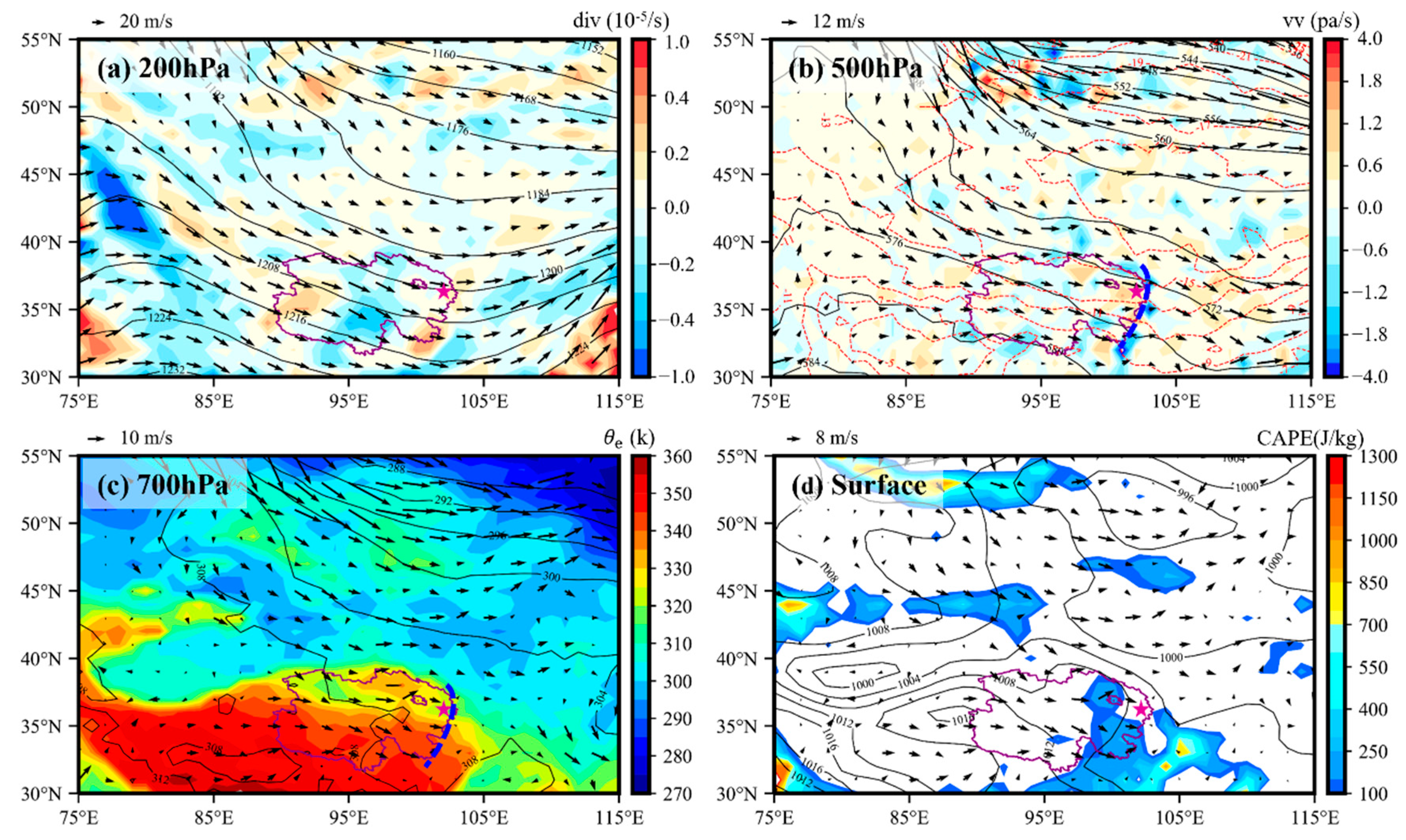
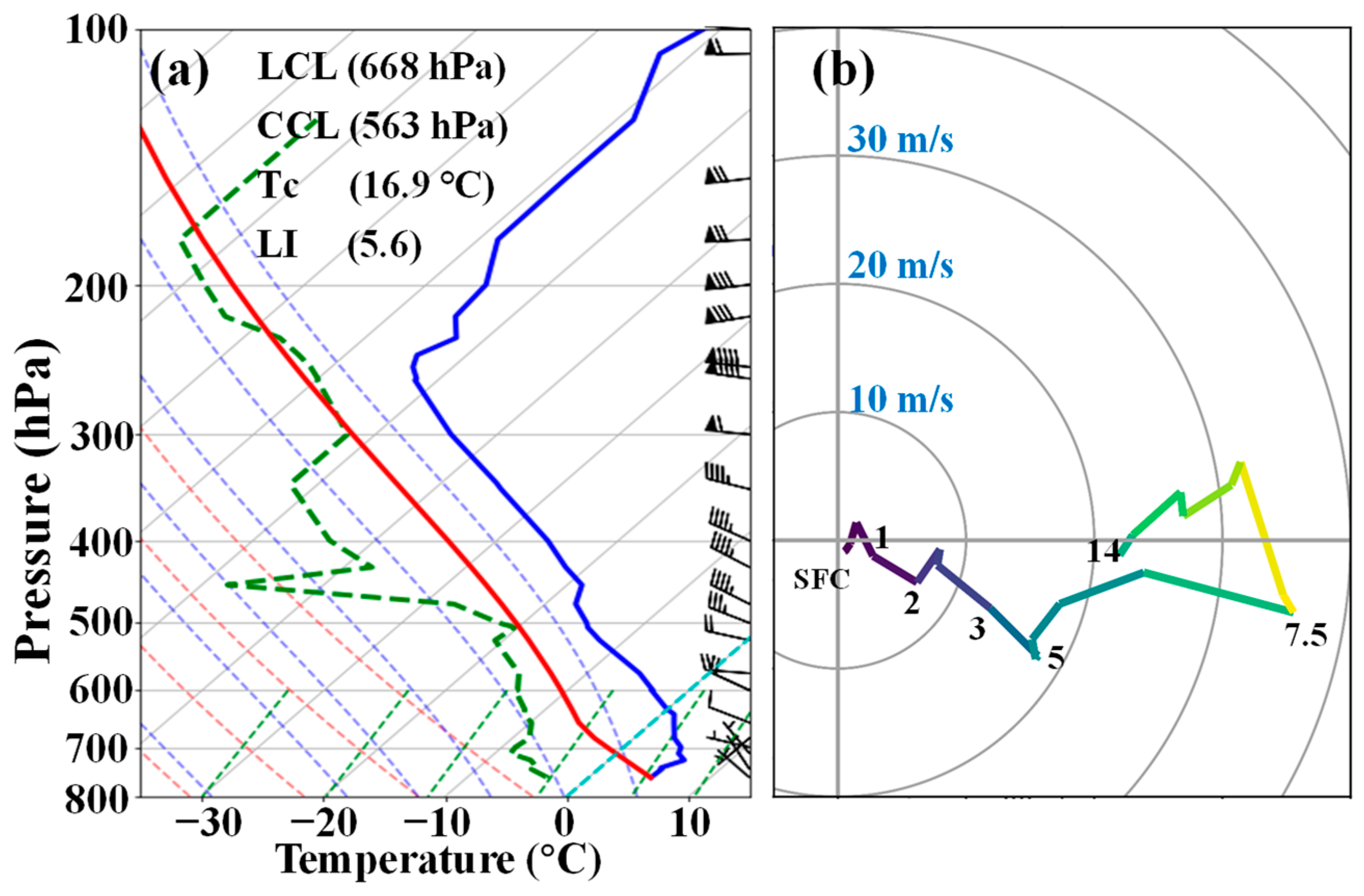
4.1. Synoptic Conditions

As the largest and highest plateau in the world, QTP is frequently covered by active cumulus in summer owing to the strong thermal and dynamic effects of the enormous terrain [25,26,27]. Under the control of local low-pressure synoptic systems, such as shear lines, troughs, and vortices, the plateau cumuli can rapidly develop and merge into MCSs [26,28]. Besides, when solar radiation produces strong thermal forcing in complex-terrain areas, the unstable atmosphere can make convection easier, such as in the northwest of Qinghai Lake [26,27], an upstream area of ZLXN (shown in Figure 1).
To investigate synoptic conditions for the formation of the MCS and microburst line, NCEP/FNL (National Centers for Environmental Prediction Final Operational Global Analysis) and radiosonde data were first analyzed. Figure 2 shows large-scale synoptic circulations at high (200 hPa), middle (500 hPa), low (700 hPa), and surface levels, superimposed by concerned atmospheric kinetic and thermodynamic variables, at 14:00 LST on 14 May 2020. In subgraphs Figure 2a–d, shaded contours denote the divergence (div, 10−5/s), vertical velocity (vv, Pa/s), equivalent potential temperature ( θ e , k), and convective available potential energies (CAPEs, J/kg).
It can be found that a deep cyclonic circulation region resided in the east of Qinghai Province, where the northwest jet controlled ZLXN (purple star) and adjacent areas at 200 hPa (Figure 2a). The divergence fields were located over Qinghai Lake and ZLXN, respectively, which were conducive to accumulating the instability energy in these areas [29]. In the middle troposphere (Figure 2b), Qinghai Province was still dominated by the northwesterly jet stream (≥20 m/s) with relatively warm air (>−13 °C). A shallow north-south oriented trough line (blue bold dotted line) was presented near ZLXN in both the middle and lower troposphere (Figure 2c). The vertical air motions on the west and east sides of the trough were downward and upward, respectively, which provided favorable dynamic conditions for the lifting of water vapor and the formation of cloud-precipitation. The strong northwesterly jet stream also prevailed around the west of the trough to facilitate the formation of a dry-air intrusion at 500 hPa. Temperature contours trended northwest-southeast in Qinghai, which were parallel to the jet stream and implied insignificant temperature advection.
From Figure 2c, we can find that θ e s (≥320 k) was relatively high over Qinghai Lake while low at ZLXN at 700 hPa level, suggesting water vapor transportation from the upstream lake to the airport. This warm moist air advection provided the synoptic-scale lifting and essential moistures to form convections [30]. Close to the surface, it can be found that ZLXN was at the edge of a weak low-pressure system which was centered near Lake Baikal. The CAPEs (≤180 J/kg) near Qinghai Lake implied weak latent instability. Although moisture and CAPEs do not strictly meet the strong convection formation criteria in the low-altitude regions to some extent, they have been proven to be favorable for the development of dry and low-reflectivity storms in plateau mountainous areas [31].
Figure 3a presents the local radiosonde profiles at 08:00 LST on 14 May 2020. Profiles of temperature and dew-point temperature indicate poor humidity conditions, especially at 450 hPa. Observations prove that a shallow dry inversion layer occurred at low level in the early morning, which tends to suppress the development of convection in the boundary layer [32]. As solar radiation heating became stronger, especially by the afternoon, the dry inversion was broken and the lapse rate of atmospheric temperature could reach or even exceed the dry adiabatic rate [33]. Meanwhile, the accumulated unstable energy and water vapor in the boundary layer were ultimately transported to the middle troposphere [34,35,36]. These thermodynamic mechanisms helped form a favorable atmospheric stratification for convective activity in the local area [12,37]. Changes in environmental wind speed can be seen from the hodograph in Figure 3b. Wind shear was mainly unidirectional in the range of 0–3 km and 0–5 km, corresponding to shear values of 12 and 17 m/s, respectively. The unidirectional vertical wind shear can be a potential sign of the follow-on dry downbursts as proposed by Dotzek and Friedrich (2009) [38] and Funk et al. (1999) [39]. Four relevant thermodynamic indexes, including LI (Lifting Index, 5.6), LCL (Lifting Condensation Level, 668 hPa, ~900 m AGL), CCL (Convective Condensation Level, 563 hPa, ~2400 m AGL), and Tc (Convective Temperature, 16.9 °C), were also calculated. It seems that the LI, LCL, and CCL did not reflect apparent potentialities for convection activity in the morning, while the low Tc implied a favorable thermal forcing lift.

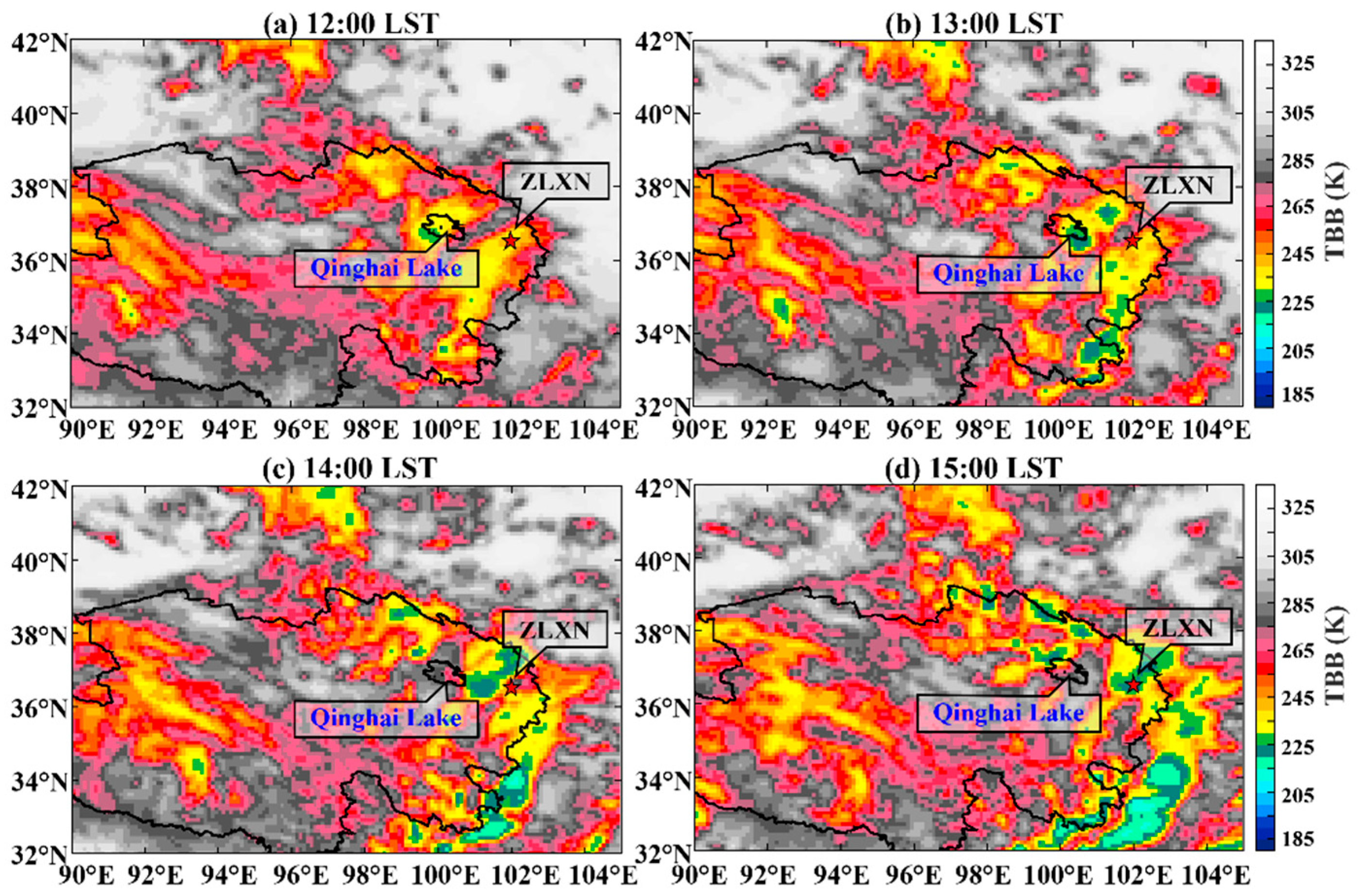
4.2. Evolutions and Structures of the MCS

The geostationary satellite FY-2G provides an overview of the macroscopic evolution of the MCS. Figure 4 shows the black body temperatures (TBBs) during 12:00–16:00 LST on 14 May 2020. The TBB images demonstrate that the MCS had generally formed, and its relevant cloud clusters had already affected ZLXN at 12:00 LST (Figure 4a). Subsequently, the convective system further developed and matured during 13:00–15:00 LST (Figure 4b–d). Clouds and precipitation rapidly became larger and stronger with lower TBBs (minimum to near 220 K) in cluster centers. The MCS generally moved from northwest to southeast. Moreover, we found that the upstream clusters that affect ZLXN are mainly intensified around the eastern edge of Qinghai Province, a windward mountainous terrain. During the convective process, Qinghai Lake also supplemented water vapors to strengthen the convection.
C-band DWR measurements were further used to characterize the storm’s intensity, evolution, and structures. Four instances of radar CRs during the MCS maturing stage are shown in Figure 5a1–d1, in which the solid black lines and squares represent the airport runway and final approach area (1 mile × 1 mile), respectively. It can be seen that, at 14:54 LST (Figure 5a1), the MCS system consists of individual small-scale storm cells, which were jointly organized to form a narrow bow echo (the thick black curves). The narrow bow echo had moved to the west terminal of the runway, with strong reflectivity gradients at the leading edge. Subsequently, the bow echo continually moved southeastward under the guidance of steering flows (Figure 5b1,c1). By 15:14 LST (Figure 5d1), it merged with several emergent cumuli and crossed over the runway and final approach areas.
Figure 5a2–d2,a3–d3 give the contemporaneous RCSs and VCSs of storms along the runway direction. In the subgraphs, the red arrows labeled with ‘A’, ‘B’, ’C’, and ‘D’ denote downdrafts produced by storm cells; the vertical dotted lines and ellipses represent the runway area and radial convergence (RC), respectively. The RCS at 14:54 LST (Figure 5a2) shows that the hydrometeor echo exhibited weak horizontal reflectivity gradients above the cloud base with apparent virga extending towards the ground. By 15:01 LST (Figure 5b2), downdrafts ‘A’ and ‘B’ were both over the runway and were separated by a distance of ~2 km. Meanwhile, a rapid descending reflectivity core corresponding to downdraft ‘C’ appeared at 800–1000 m above ground level (AGL), and ~3 km away from the airport. Note that the RCs in Figure 5b3, which have been reported to play a vital role in the formation and development of downbursts [39], were both under 1.5 km AGL. Their observed heights are much lower than the heights of so-called mid-altitude radial convergences (MARCs) found in windstorms in plain areas [40,41]. As another indicator of microbursts, the hanging virga echoes rapidly break out from low-reflectivity storm cells, as pointed out by the red arrows in Figure 5a2,d2. This phenomenon seems to be the same as that observed in other plateau areas and is perceived to be particularly hazardous to aviation activity [6,12,42]. At 15:08 LST (Figure 5c2,3), we can find that downdrafts ‘A’, ‘B’, and ‘C’ had already touched the ground, and ‘C’ was stronger than both ‘A’ and ‘B’. Moreover, a combination of RC and radial divergence (RD) can be observed, which were very prominent to reflect the wind radial characteristics of the downburst outflows. By 15:14 LST (Figure 5d2,3), downdrafts ‘A’ and ‘B’ merged and passed the runway; however, ‘C’ still affected the right terminal of the runway. Meanwhile, an upcoming downburst of ‘D’ seems to burst at ~7-km away from the left terminal of the runway.
The storms and downbursts led to drastic changes in meteorological elements around the runway. According to the observatory records, the cumulonimbi cloudage was up to 5/8 (8 represents the cloudage of a full sky) when storms approached the airport. Figure 5 shows the time series of horizontal winds, sea-level atmospheric pressures, and temperatures observed by the AWOSs on the runway during 14:30–15:30 LST. It shows that wind speeds on W#AWOS (which denotes the west AWOS on the runway, Figure 6a) and E#AWOS (which denotes the east AWOS on the runway, Figure 6b) sharply increased from 6 m/s to 15 m/s and from 5 m/s to 18.5 m/s, respectively, during 14:30–15:00 LST. Initially, wind directions on RWYs were westerly, but they subsequently rotated clockwise to northerly on W#AWOS and northwesterly on E#AWOS, respectively. By 15:20 LST, wind directions on W#AWOS rotated almost 180°, while those of E#AWOS still maintained northwesterly, indicating a wind field diversion on the runway. All these wind variations react to low-level wind shear [13]. Furthermore, it can be observed from Figure 6c that a decrease of 3.5 °C in temperature and an increase of 3 hPa in query normal height pressure (QNH pressure, which indicates the barometric pressure at sea level) [43] due to the drag effect of virga and the evaporation effect of storm downflows in the dry and warm environment [7]. Additionally, the total rain amount measured by rain gauges on the runway was less than 0.1 mm.

4.3. Variations, Structures, and Evolutions of the Dry Microburst Line and Wind Fields

The scanning DWL can provide more sophisticated and comprehensive wind measurements than the C-band weather radar and AWOSs, especially under non-precipitating or fair-weather conditions. In this subsection, multiple DWL scanning data were further utilized to explore the variations, structures, and evolutions of the dry microburst line and relevant wind fields from various perspectives.

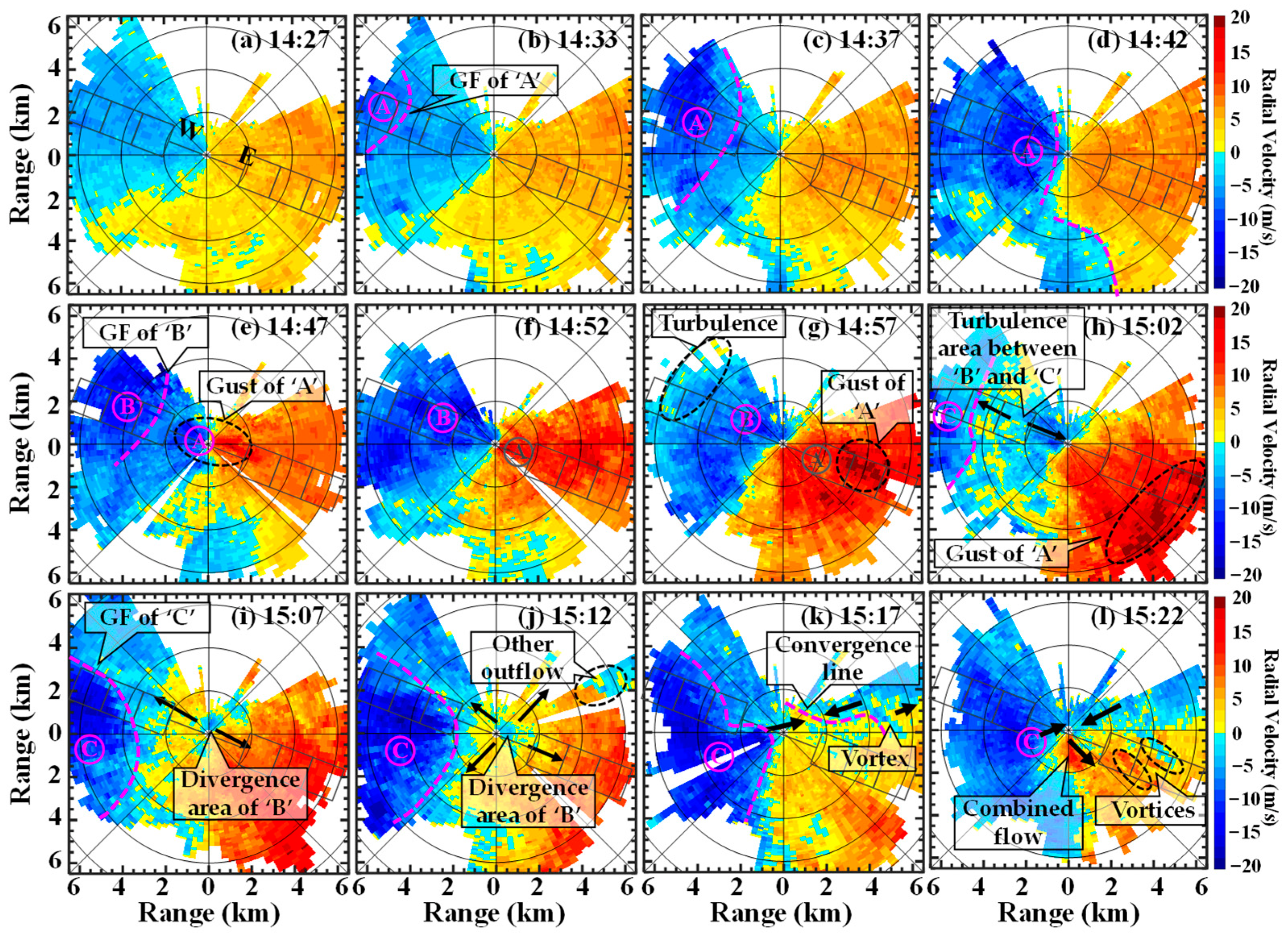
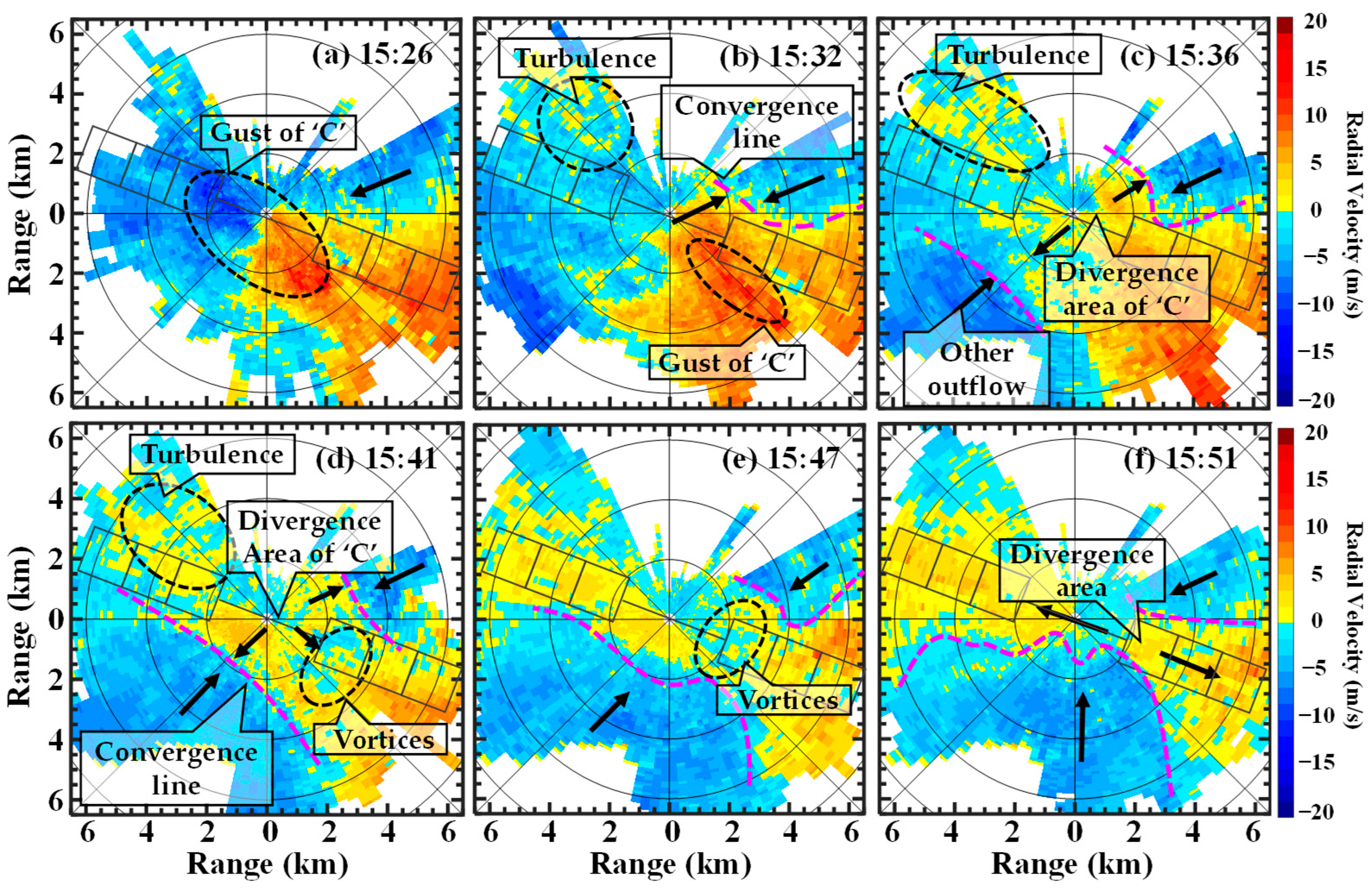
4.3.1. Horizontal Perspectives

To recognize the horizontal characteristics of microbursts and relevant winds, 5 min-interval DWL PPI images of radial velocity from 14:27 to 15:51 LST are drawn in Figure 7 and Figure 8. It can be seen that, before the approach of storms (Figure 7a), ambient winds around the airport were generally northwesterly with small radial speeds of 0–5 m/s. Until 14:33 LST (Figure 7b), outflows (enclosed alphanumerics) and a gust front (GF) (the purple dotted line) produced by the downburst ‘A’ first intruded the corridor with strong northwesterly winds (>10 m/s). As the outflows of ‘A’ gradually moved to the DWL (Figure 7c,d), the divergent gale expanded and the radial wind speeds on RWY-W reached 20 m/s at 14:42 LST. In addition, southerly outflows from other convections also yielded a convergence line (the purple dotted line) located 3–6 km south of the DWL. Five minutes later (Figure 7e), a pair of large radial speed centers (the black dotted ellipse) appeared on both sides of the DWL, implying the outflows of downburst ‘A’ were passing through the runway. Meanwhile, another well-developed downburst of ‘B’ had also spread to the northwest of the site. Furthermore, outflows of downburst ‘A’ and ‘B’ coalesced to form a larger gale area, nearly covering the entire runway and both sides of the corridor at 14:52 LST (Figure 7f). Meanwhile, there formed a weak, unidirectional uniform airflow between ‘A’ and ‘B’ (between the purple dotted line and the black dotted ellipse). Until 14:57 LST, the gale area of two downbursts continually moved southeastward, and two apparent turbulent areas appeared on both sides of the corridor (the dotted ellipses in Figure 7g) due to the interaction of downbursts and the influences of complex terrain. This observational finding is consistent with the simulation results of Orf et al. (1996) [15] and Vermeire et al. (2011) [16].
In the next 25 min, the third downburst of ‘C’ successively affected the airport. By 15:02 LST (Figure 7h), the gust leading edge of downburst ‘C’ appeared with large radial speeds in the west of the corridor. The junction area between downbursts ‘B’ and ‘C’ was the center of collision regions of turbulence [15,16], in which winds seemed to be disorderly. During 15:07–15:17 LST (Figure 7i–k), the divergence center of ‘B’ had gradually passed the runway and further moved southeastward. At the same time, outflows of ‘C’ further burst and yielded a larger divergent gale area, blocking the continued westward extension of outflows of ‘B’. Whereas as ambient flows changed from northwesterly to northerly (see AWOS results in Figure 6a), the divergent gale subsequently moved southwesterly and approached the DWL site. By 15:22 LST (Figure 7l), interestingly, the airport was controlled mostly by inflows in the first three quadrants but by outflows in the fourth quadrant. In addition, there existed several streak-shaped flows on the east side of the corridor (the dotted ellipses), which may be caused by horizontal roll vortices as proposed by Etling et al. (1993) [44] and Brown et al. (1980) [45].
Winds resumed blowing northwesterly and calmed down to some extent at 15:26 LST (Figure 8a) when outflow fronts of ‘C’ passed the site. Until 15:32 LST (Figure 8b), turbulences (the dotted circle) appeared in the northwest again, which may be related to the downburst ‘D’. Meanwhile, a convergence line (the purple dotted lines) can be found in the northeast as a result of the collision between ‘C’ and outflows from other northeastern windstorms. The divergent center of ‘C’ appeared at 15:36 LST (Figure 8c). In the third quadrant, a relatively longer convergence line was also formed by the intrusion of southwesterly outflows from other convections (the purple dotted line). It was found that the turbulence area caused by ‘D’ was expanding northwesterly. Under the joint impact of the above-mentioned outflows from different directions, wind fields changed more complicatedly during the next 10 min. At 15:41 LST (Figure 8d), wind speeds generally weakened to a large extent. In addition, the northeasterly outflows created a barrier in the movement direction of ‘C’. They squeezed ‘C’ together with southwesterly outflows, resulting in two velocity pairs resembling roll vortices in the front of ‘C’ (the southeast dotted ellipses). By 15:47 LST (Figure 8e), northwest turbulences faded away and the ‘C’ had moved to the end of RWY-E. As two strong inflows (from the northeast and south) approached, the vortices structure remained, whereas its size became smaller than before. At 15:51 (Figure 8f) LST, the vortices gradually decayed because of the extrusion of two robust inflows. However, these two inflows did not further erode due to the resistance of the ‘C’ legacy wind fields, which formed a band-shape divergent area over the whole runway. Under these circumstances, although wind speeds are relatively weak, they can produce wind shear in several directions and pose a significant potential danger to the aircraft. The entire microburst line process lasted for ~90 min and had a strong sense of turbulence with several sudden changes in wind fields. When all the convections left the airport, those winds finally calmed down after 16:05 LST.

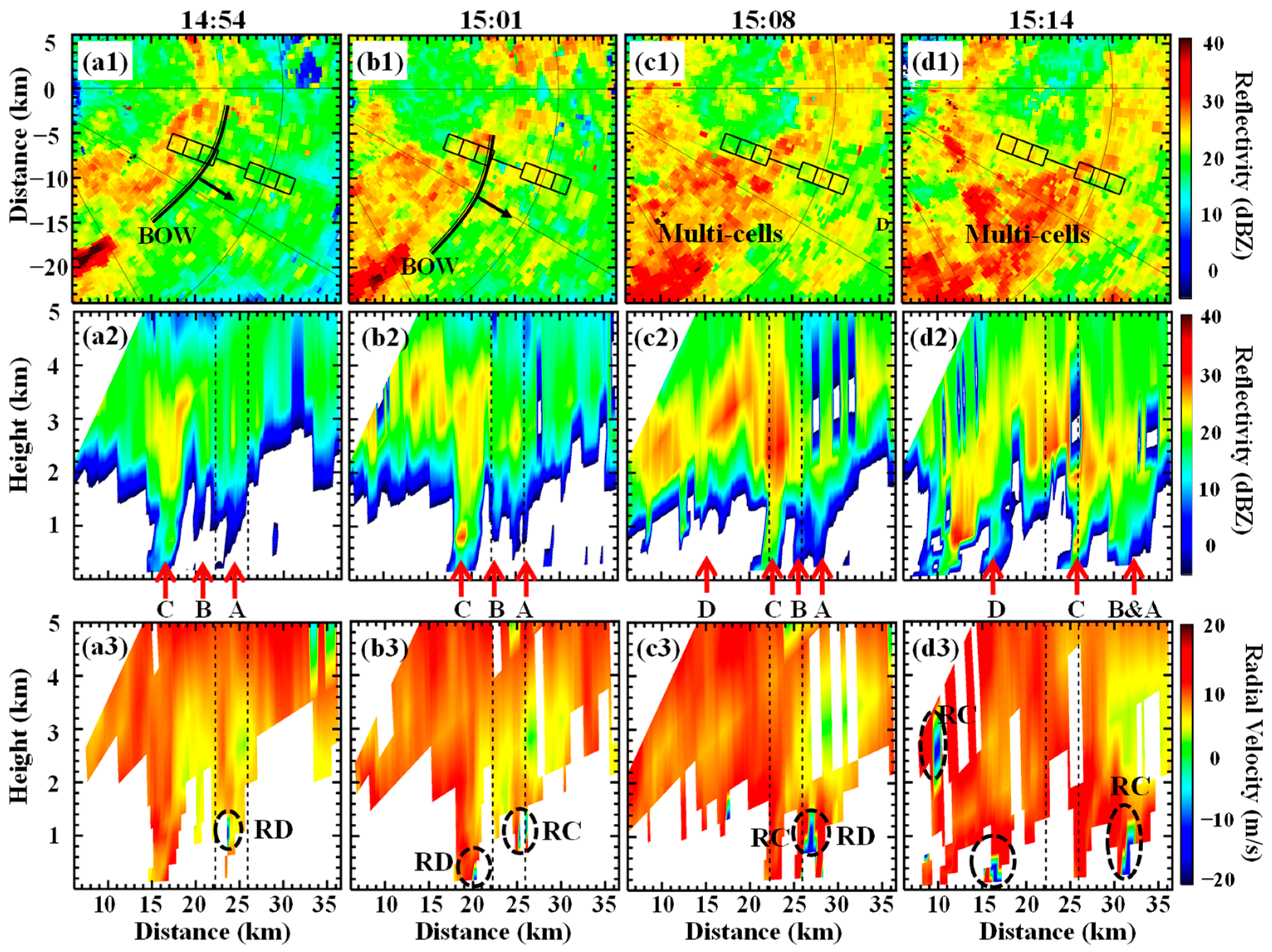
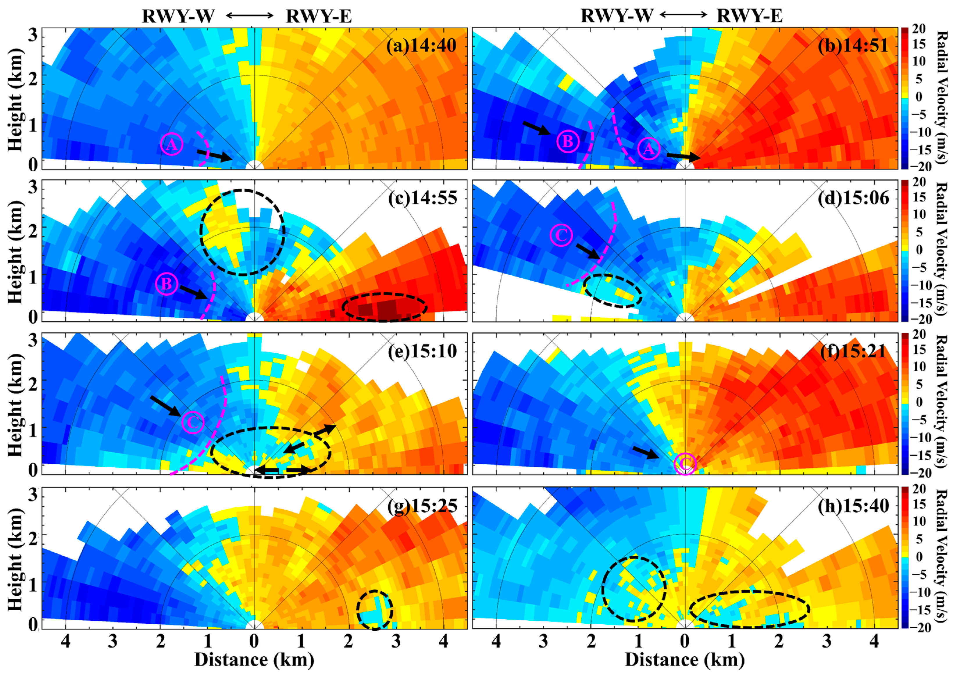
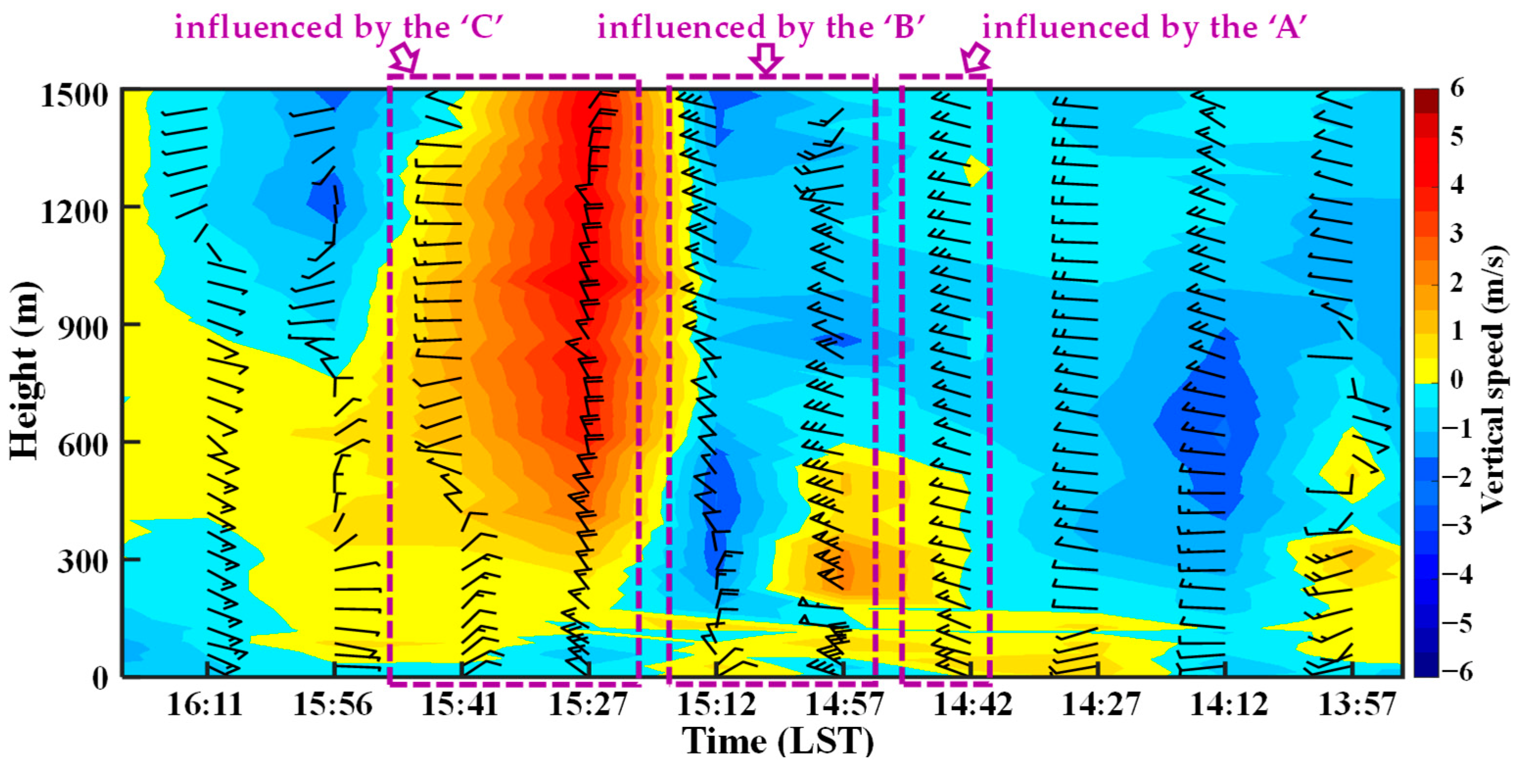
4.3.2. Vertical Perspectives

We analyzed the DWL RHI and DBS measurements to investigate the characteristics of downbursts and relevant wind fields from vertical perspectives in this section. Figure 9 presents eight RHI panels of radial velocity aloft on the runway during 14:40–15:40 LST. It can be observed that, at 14:40 LST (Figure 9a) (before the invasion of downburst ‘A’), ambient winds at low levels were homogeneous and relatively weak in general. As the outflows of ‘A’ gradually descended and spread to the near ground, radial winds became faster with a maximum speed of ~15 m/s. Note that there is a lack of measurements from 90° to 140° due to the laser attenuation caused by clouds and precipitation. Until 14:51 LST (Figure 9b), outflows of ‘B’ followed ‘A’ from the northwest with a space interval of ~1 km, and the coalescence region under 1 km, between two downbursts (the junction between the two purple dotted lines) was distinctly visible. Four minutes later (Figure 9c), the DWL captured an “adverse wind area” aloft the site (the dotted circle), which corresponds to the RD observed by DWR as shown in Figure 5a3. Meanwhile, even stronger radial winds exceeding 19 m/s appeared at the front of ‘A’. Until 15:06 LST (Figure 9d), a transparent shear layer appeared at 1 km ASL since the front of ‘C’ was still perched in the air. Due to the absence of measurements from 169° to 177°, the turbulence zone (the dotted ellipse) was not noticeable. By 15:10 LST (Figure 9e), the front of ‘C’ downed to low levels from 1 km to 0.5 km with wind speeds of ~10–15 m/s. In addition, near the site, a divergence area exhibited by vortices structures (the dotted ellipse and black arrows), of which the horizontal extent was near 2.5 km, can be found due to the interaction between the outflows of ‘C’ and ambient winds. After ten minutes (Figure 9f), the vortices disappeared, and ‘C’ finally touched the ground and then passed the site to make the radial winds asymmetrically distributed. As ‘C’ further propagated eastward, a residual vortex circulation (the dotted ellipse) can be seen near RWY-E at 15:25 LST (Figure 9g). Until 15:40 LST (Figure 9h), outflows from all convections generally dissipated or moved out, and ambient winds gradually calmed down. In contrast, divergent and turbulent areas (the dotted ellipse and circle) near the surface may still be hazardous for the following aircraft.
Figure 10 shows a time-height profile of horizontal and vertical winds observed by the DWL DBS mode at a distance of under 1.5 km during the period of 13:57–16:11 LST. Specifically, before 14:27 LST, horizontal winds (wind barbs) were mostly westerly with speeds of 2–8 m/s. Vertical air motions (shaded contours) were very weak and mostly downward. Until 14:42 LST, as the front of downburst ‘A’ initially approached the site, horizontal winds mainly changed from westerly to northwesterly with an increase of 2–4 m/s. A weak updraft of nearly 550 m was also observed as the cool downburst outflows embedded and lifted the warm ambient airflows. Subsequently, by 14:57 LST, outflows of downburst ‘B’ invaded the site to significantly strengthen horizontal winds, especially those within 130–420 m height. The horizontal gales can be up to 20–26 m/s. Furthermore, the lower part of updrafts at this moment had been disturbed to some extent under 200 m, whereas the motion center near 300 m had strengthened. After 15 min, the horizontal winds greatly calmed down with speeds only within 2–4 m/s, while wind directions under 400 m changed to be northerly or northeasterly since the residual of downburst ‘B’ had just moved to the northeast side of the DWL (Figure 7j). The vertical winds exhibited a slight counterclockwise rotation, indicating a weak cold advection dominated the vertical motions. By 15:27 LST, downburst ‘C’ weakened and just passed the DWL site (Figure 8a), and the in situ winds were jointly influenced by the outflows from ‘C’ and other northeast convections, resulting in northerly or northwesterly horizontal winds. The horizontal winds had a general trend of a clockwise rotation from ground to air, corresponding to a warm advection, corresponding to a strong and profound updraft simultaneously observed by the DWL. In the next 20 min, as the residual of downburst ‘C’ further moved eastward, the in situ horizontal winds changed to be weak northeasterly under 600 m and maintained westerly within 600 m–1.5 km. After 15:56 LST, stable eastern flows gradually controlled the boundary layer.

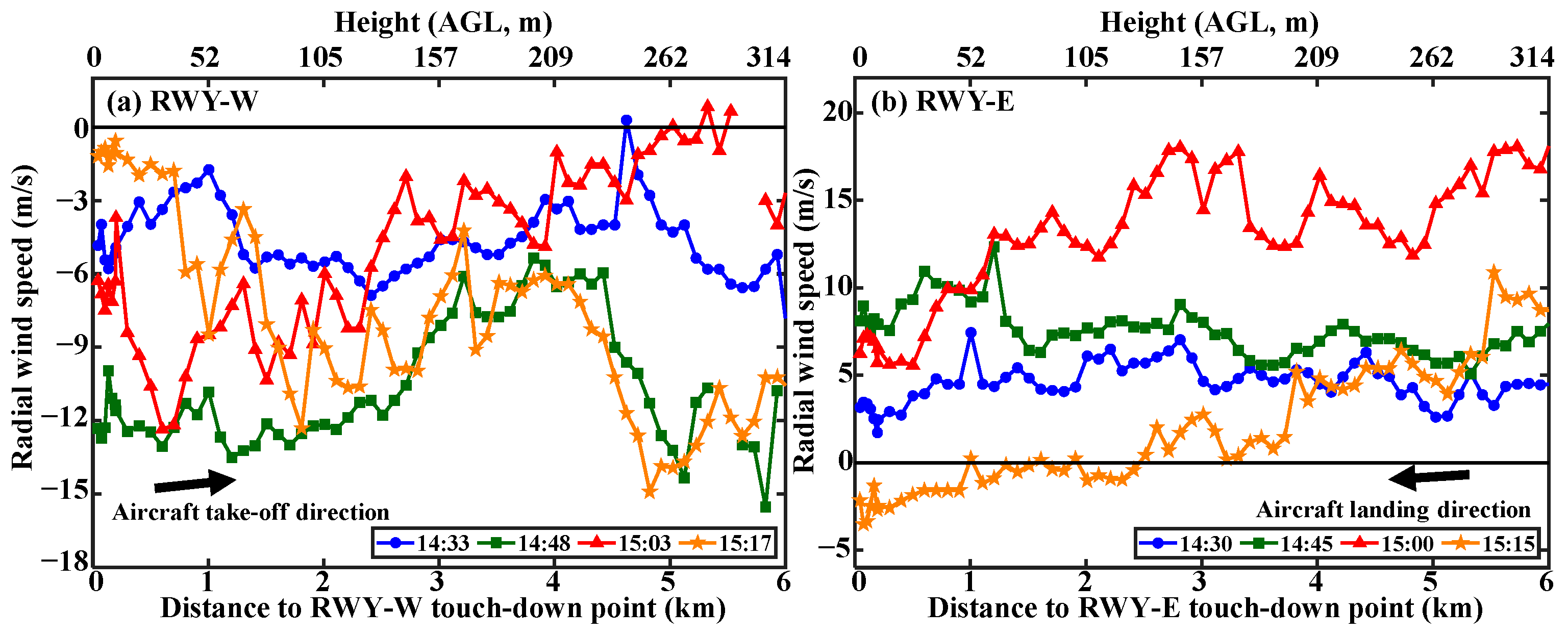
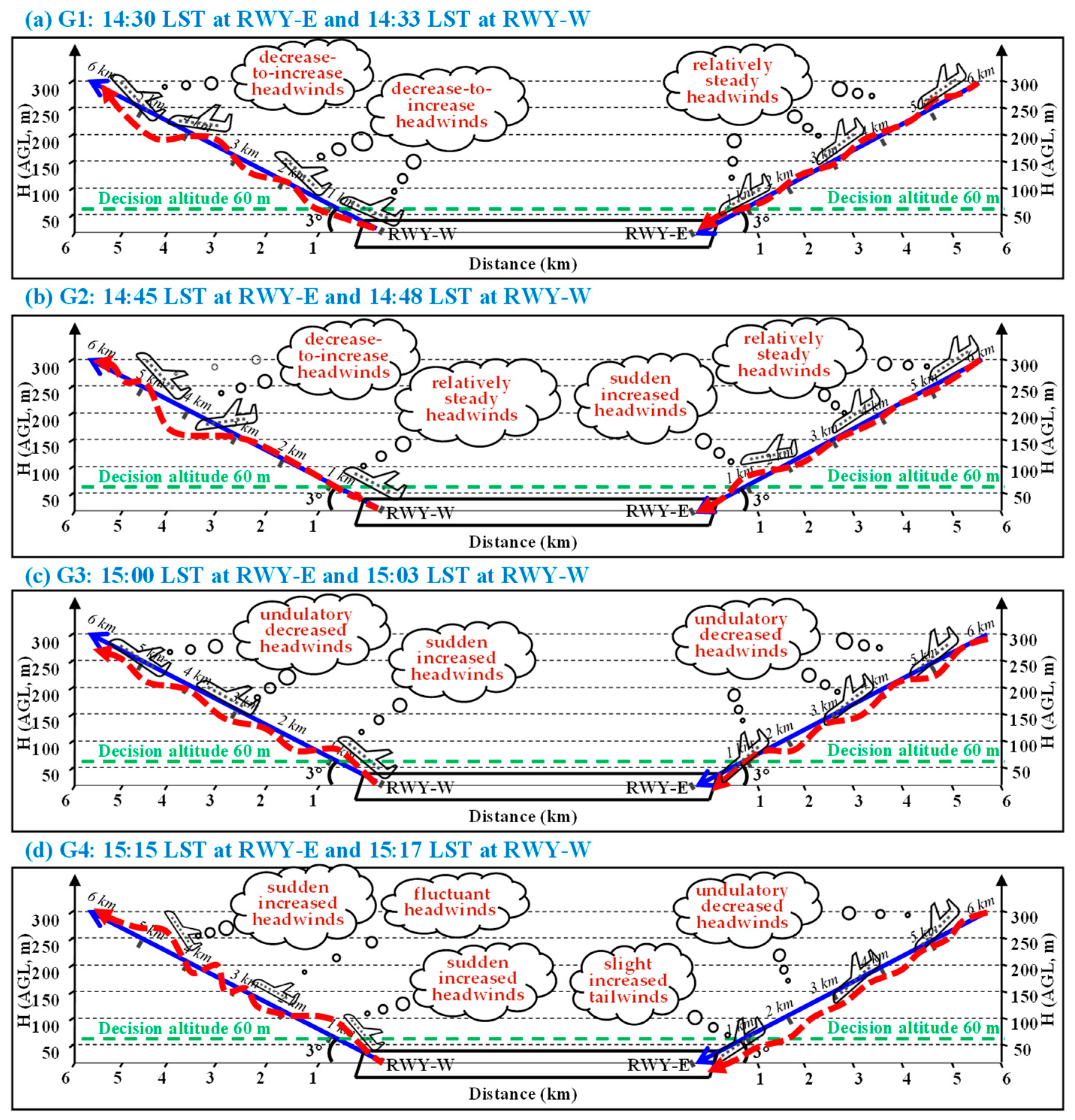
4.3.3. Glide-Path Perspectives

For civilian aircraft, descending and taking off through glide paths can be the most dangerous moments of the flight. Hence, wind changes along two glide paths observed by the DWL were further analyzed to investigate wind shear caused by the downburst activity along two glide paths of ZLXN and possible influences on aircraft. As the DWL was operated by a multi-mode combined scanning strategy, only eight instances of GP data were available during the impact period of downbursts, which herein were divided into four temporal groups as listed in Table 2. Figure 11 shows the radial wind speeds of the four temporal groups. Although the whole process is complicated, the surface wind was still dominated by northwest flows according to AWOSs (Figure 6). Thus, herein, the aircraft was assumed to land at RWY-E and depart from RWY-W by obeying a headwind condition. As aircraft gradually fly away from or land on the runway, distances from the corridor to touch-down points and heights above the ground level vary from 6 to 0 km and from 314 to 0 m (the angle between the glide path and horizontal level was assumed to be three degrees), respectively. We also plotted a schematic drawing (Figure 12) to show the aircraft trajectory and states during the take-off and landing phase under four circumstances, i.e., G1–G4. In Figure 12, the solid blue lines represent ideal aircraft trajectories, and the red curves denote actual aircraft trajectories under the influence of different radial winds. The cloud-shape annotations describe the details of wind changes.
From Figure 11 and Figure 12a, it can be seen that, for G1, radial winds along the glide path over RWY-W (take-off process) fluctuated within −8–0 m/s before the approach of downburst ‘A’. Meanwhile, the decreased headwinds near 1.2 km (almost close to a decision altitude of 60 m for pilots) pulled up the flight trajectories, and prominent decrease-to-increase speeds at 4–6 km made the aircraft suddenly fall and rise. The counterparts along the glide path over RWY-E (landing process) were within 2–7 m/s with relatively small fluctuations. Hence, aircraft would generally descend under steady headwinds and be able to land at the touch-down point. For G2 (Figure 12b), radial winds along glide paths have been dominated by outflows of downbursts ‘A’ and ‘B’. When the aircraft took off through the glide path over RWY-W, it was first influenced by steady headwinds with a speed of ~12 m/s before 1.5 km but then underwent decrease-to-increase speeds at 2.5–5 km. For the landing that took place through the glide path over RWY-E, the aircraft experienced increased headwinds within 1.5–1.1 km with increased lift, and its final touchdown position would be slightly in front of the anticipated point.
For G3 (Figure 12c), downbursts ‘B’ and ‘C’ jointly controlled radial winds along two glide paths. The aircraft generally suffered from undulatory decrease-to-increase headwinds when taking off through the glide path over RWY-W within 0–0.8 km and then encountered a gradually decreasing headwind on the rest of the way. The aircraft would undergo undulatory headwinds along the glide path over RWY-E within 6–3 km. Subsequently, it can immediately encounter consecutively decreasing headwinds and touch the ground behind the scheduled landing point. For G4 (Figure 12d), radial winds along the glide path over RWY-W were dominated by outflows of downburst ‘C’, while counterparts along the glide path over RWY-E may be jointly influenced by outflows of downburst ‘B’ and other northerly convections. When aircraft depart from the glide path over RWY-W, wind conditions may be inappropriate, and headwinds from surface to 6 km can fluctuate significantly (0 to 4 km) to severely (4 to 5 km), affecting the aircraft’s trajectory and state. Radial winds along the glide path over RWY-E indicate that aircraft would first experience undulatory decreased headwinds during 6–2.5 km and then immediately undergo slightly increased tailwinds in the lower levels. Thus, the actual touchdown position of the aircraft will be much behind the expected point.
Note that the actual aircraft experience can be more complicated than the previously mentioned wind conditions. Herein, other influencing factors, such as flight speed, planeload, aircraft types, human intervention, etc., are not considered.

5. Discussion

Due to the lack of observation networks and the harsh natural environment, small-scale convections, and downbursts over QTP have been rarely investigated and understood by meteorologists. In this work, the observational characteristics of downbursts like this one that happened in ZLXN (the QTP of China) were compared with the results obtained on the Denver plateau in the U.S. [11]. Comparisons suggest that dry downbursts in these two high-altitude regions both occurred in the afternoon under dry atmospheric conditions. Local radiosonde profiles exhibit similar observational features in the early morning, namely, the existence of a dry-adiabatic atmosphere and a shallow temperature inversion. As the strong solar radiation heated the plateau, shallow temperature inversions both broke in the afternoon to facilitate the formation and development of convections [12,46]. Vertical shears of horizontal winds are also prerequisites for the downburst formation. However, they are more apparently found in the QTP, which may be more conducive to the maintenance and organization of the downburst line by momentum propagation and hydrometeor evaporation [47,48,49].
The observational features and variations of storms and downbursts by the DWR in this study, including bow-shape echoes, descending reflectivity cores, RCs, and RDs, are also similar to the results of a conceptual model proposed by Roberts et al. (1989) [41] and other outcomes in studies within the literature [4,37,50]. Although not all of the DWR features in this study are identical in spatial terms to other research, such as the heights of RCs being lower than those in plain areas [40,41], these standard features hint that the radar observations based on our work and previous literature can be helpful for dry downbursts forecasting and warning in the eastern QTP.
The evolution of low-level winds for this downburst line event is eventually summarized in conceptual models drawn in Figure 13. The downburst line begins with a gust front and is successively joined by the other two following microbursts. Consistent with the findings of Parsons and Kropfli (1990) [48], the GF of ‘A’ does not contain horizontal roll vortices at the leading edge and may indicate a lack of strong downdrafts below 1 km (Figure 10). In addition, the adjacent interaction between downbursts ‘A’ and ‘B’ makes the variation of near-surface wind fields similar to simulation results of complex interaction and coalescent patterns of downbursts reported by Orf et al. (1996) [15] and Vermeire et al. (2011) [16]. Moreover, our integrated observations by multiple sensors can actually reveal more dynamics and thermodynamics details: (1) The frontal outflows of downburst ‘B’ may undercut the backward outflows of ‘A’ and reorder the shape of the coalescent area as weak and one-way uniform airflows (as shown in Figure 13a); (2) according to Figure 13b, ‘B’ causes a complete divergence as the following ‘C’ keeps an appropriate distance. Meanwhile, the divergence area of ‘B’ and the outflows of ‘C’ together yield a turbulent region under complex interaction factors; (3) as presented in Figure 13c, outflows of ‘C’ are captured and invaded by inrush flows from other directions; (4) the combined flows change the moving direction of ‘C’ and trigger the horizontal vortices at its front; and (5) it is apparent from Figure 13d that complex interactions, driven by multi-outflows, are responsible for the formation of unique small-scale outflow features, such as changing the divergence area shape of ‘C’ and triggering small vortices.

6. Conclusions

The QTP possesses frequent convective activities owing to its special dynamic and thermal effects on the atmosphere, and the civilian airplane has been the most important mode of transportation for the local people. However, to date, only rare studies or investigations have paid enough attention to the small-scale downbursts over this high-altitude region. To better understand dry downburst events over QTP and explore the synergetic usage of different remote sensing technologies for downburst detection and warning in the airport terminal, this study describes and interprets a typical traveling low-reflectivity dry microburst line that happened at ZLXN on 14 May 2020. Specifically, characteristics of synoptic conditions, the MCS formation process, and the structure and evolution of downbursts and their low-level winds were comprehensively analyzed. The main findings can be concluded as follows.
The microburst line consists of three individual dry microbursts and persists for nearly 90 min. During this process, gales can exceed 18 m/s and cause hazardous low-level wind shear, resulting in the go-around of an arriving aircraft. Before the formation of storms and downbursts, synoptic conditions and radiosonde characteristics observed near ZLXN are found to be similar to counterparts obtained in Denver, U.S., even though the climates and geographic locations of the two regions are different. Specifically, the deep, dry boundary layer may favor evaporative cooling and melting of precipitation that create negative buoyancy [51]. These features enabled the ZLXN microburst line to be driven and maintained with the support of strong vertical shears of horizontal winds. For windstorms, the DWR reflectivity during the observation period exhibited a gradual progression from narrow bow-shape echo (associated with strong gusts) to multi-cell convections. Furthermore, the descending airflows are mostly associated with descending high reflectivity cores, RCs, and RDs.
The interactive outflows between downbursts exhibit different features. When downdrafts hit the ground, significant turbulence and radial divergences were observed in the lowest few hundred meters. During or after outflows colliding, the DWL spotlighted the evolution of roll vortices and discontinuity of radial speed in a high spatiotemporal resolution. The DWL captured the unique features of horizontal downburst outflows and their collision effects, which are high-speed burst swaths, turbulences, divergence regions, convergence lines, and vortices. The manifestations of low-level wind shear in PPI and RHI scans can be considered a critical validation and supplement of previous simulation results [15,16].
From the perspective of aviation safety, compared with an isolated downburst, the downburst line can enlarge the damaging lifetime, footprints, and prediction difficulty. This study demonstrates that a synergy of various types of real-time detection devices can help to monitor and warn of the occurrence of downbursts and concomitant wind shear. In the future, other downbursts will be investigated similarly to categorize the meteorological situations and observational signs that are conducive to downburst formation in plateau areas. In addition, research on the automatic identification and warning algorithms for downbursts and wind shear is also of significant necessity.

Author Contributions

Conceptualization, X.H. and J.Z.; methodology, X.H. and Y.C.; software, X.H., and T.R.; validation, X.H. and Y.C.; formal analysis, X.H.; investigation, J.Z. and G.W.; resources, J.Z.; data curation, Z.H. and W.T.; writing—original draft preparation, X.H.; writing—review and editing, J.Z. and Y.C.; visualization, X.H. and J.Z.; supervision, J.Z., and Z.S.; project administration, J.Z., and L.S.; funding acquisition, J.Z. and Y.C. All authors have read and agreed to the published version of the manuscript.

Funding

This research was funded by the National Key Research and Development Program of China (Grant No. 2021YFC3001902) and the National Natural Science Foundation of China (Grant No. 41905084).

Institutional Review Board Statement

Not applicable.

Informed Consent Statement

Not applicable.

Data Availability Statement

Not applicable.

Acknowledgments

The authors would like to thank the reviewers for their thorough comments that helped to improve the manuscript.

Conflicts of Interest

The authors declare no conflict of interest.

References

  1. Fujita, T.T. The downburst. SMRP 1985, 210, 112. [Google Scholar]
  2. Solari, G. Thunderstorm downbursts and wind loading of structures: Progress and prospect. Front. Built Environ. 2020, 6, 63. [Google Scholar] [CrossRef]
  3. Wakimoto, R.M. Convectively driven high wind events. In Severe Convective Storms; Springer: New York, NY, USA, 2001; pp. 255–298. [Google Scholar]
  4. Fujita, T.T. Tornadoes and downbursts in the context of generalized planetary scales. J. Atmos. Sci. 1981, 38, 1511–1534. [Google Scholar] [CrossRef] [Green Version]
  5. Hawbecker, P.S. The Influence of Ambient Stability on Downburst Winds. Available online: https://www.proquest.com/openview/8bf62d3b131104a6906af6654740dd52/1?pq-origsite=gscholar&cbl=18750 (accessed on 1 June 2022).
  6. Wilson, J.W.; Roberts, R.D.; Kessinger, C.; McCarthy, J. Microburst wind structure and evaluation of Doppler radar for airport wind shear detection. J. Appl. Meteorol. Climatol. 1984, 23, 898–915. [Google Scholar] [CrossRef] [Green Version]
  7. Proctor, F.H. Numerical simulations of an isolated microburst. Part II: Sensitivity experiments. J. Atmos. Sci. 1989, 46, 2143–2165. [Google Scholar] [CrossRef] [Green Version]
  8. Fujita, T.T. Downbursts and microbursts-An aviation hazard. In Proceedings of the Conference on Radar Meteorology, Miami Beach, FL, USA, 1 January 1980. [Google Scholar]
  9. Fujita, T.T. Microbursts as an aviation wind shear hazard. In Proceedings of the 19th Aerospace Sciences Meeting, St. Louis, MO, USA, 12–15 January 1981; p. 386. [Google Scholar]
  10. Wilson, J.W.; Wakimoto, R.M. The discovery of the downburst: TT Fujita’s contribution. Bull. Am. Meteorol. Soc. 2001, 82, 49–62. [Google Scholar] [CrossRef]
  11. Caracena, F.; Flueck, J. Forecasting and classifying dry microburst activity in the Denver area subjectively and objectively. In Proceedings of the 25th AIAA Aerospace Sciences Meeting, Reno, NV, USA, 24–26 March 1987; p. 443. [Google Scholar]
  12. Wakimoto, R.M. Forecasting dry microburst activity over the high plains. Mon. Weather Rev. 1985, 113, 1131–1143. [Google Scholar] [CrossRef] [Green Version]
  13. Hjelmfelt, M.R. Structure and life cycle of microburst outflows observed in Colorado. J. Appl. Meteorol. Clim. 1988, 27, 900–927. [Google Scholar] [CrossRef]
  14. Hjelmfelt, M.R. The microbursts of 22 June 1982 in JAWS. J. Atmos. Sci. 1987, 44, 1646–1665. [Google Scholar] [CrossRef] [Green Version]
  15. Orf, L.G.; Anderson, J.R.; Straka, J.M. A three-dimensional numerical analysis of colliding microburst outflow dynamics. J. Atmos. Sci. 1996, 53, 2490–2511. [Google Scholar] [CrossRef] [Green Version]
  16. Vermeire, B.C.; Orf, L.G.; Savory, E. A parametric study of downburst line near-surface outflows. J. Wind Eng. Ind. Aerodyn. 2011, 99, 226–238. [Google Scholar] [CrossRef]
  17. Tse, S. Optimization of terminal Doppler weather radar at Hong Kong international airport for microburst detection. In Proceedings of the 9th European Conference on Radar and Meteorology and Hydrology, Antalya, Turkey, 10–14 October 2016. [Google Scholar]
  18. Ozdemir, E.T.; Deniz, A.; Sezen, I.; Aslan, Z.; Yavuz, V. Investigation of thunderstorms over Ataturk International Airport (LTBA), Istanbul. Mausam 2017, 68, 175–180. [Google Scholar] [CrossRef]
  19. Adachi, T.; Kusunoki, K.; Yoshida, S.; Arai, K.-I.; Ushio, T. High-speed volumetric observation of a wet microburst using X-band phased array weather radar in Japan. Mon. Weather Rev. 2016, 144, 3749–3765. [Google Scholar] [CrossRef]
  20. Burlando, M.; Romanić, D.; Solari, G.; Hangan, H.; Zhang, S. Field data analysis and weather scenario of a downburst event in Livorno, Italy, on 1 October 2012. Mon. Weather Rev. 2017, 145, 3507–3527. [Google Scholar] [CrossRef]
  21. Zheng, Y.; Chen, J.; Zhu, P. Climatological distribution and diurnal variation of mesoscale convective systems over China and its vicinity during summer. Sci. Bull. 2008, 53, 1574–1586. [Google Scholar] [CrossRef] [Green Version]
  22. Haines, D.A. Downbursts and Wildland Fires: A Dangerous Combination. Available online: https://www.fs.usda.gov/sites/default/files/fire-management-today/64-1.pdf#page=59 (accessed on 1 June 2022).
  23. Intrieri, J.M.; Bedard, A.J., Jr.; Hardesty, R.M. Details of colliding thunderstorm outflows as observed by Doppler lidar. J. Atmos. Sci. 1990, 47, 1081–1099. [Google Scholar] [CrossRef] [Green Version]
  24. Nechaj, P.; Gaal, L.; Bartok, J.; Vorobyeva, O.; Gera, M.; Kelemen, M.; Polishchuk, V. Monitoring of low-level wind shear by ground-based 3D lidar for increased flight safety, protection of human lives and health. Int J. Environ. Res. Public Health 2019, 16, 4584. [Google Scholar] [CrossRef] [Green Version]
  25. Yanai, M.; Li, C. Mechanism of heating and the boundary layer over the Tibetan Plateau. Mon. Weather Rev. 1994, 122, 305–323. [Google Scholar] [CrossRef]
  26. Guofu, Z.; Shoujun, C. Analysis and comparison of mesoscale convective systems over the Qinghai-Xizang (Tibetan) Plateau. Adv. Atmos. Sci. 2003, 20, 311–322. [Google Scholar] [CrossRef]
  27. Sugimoto, S.; Ueno, K. Formation of mesoscale convective systems over the eastern Tibetan Plateau affected by plateau-scale heating contrasts. J. Geophys. Res. 2010, 115. [Google Scholar] [CrossRef]
  28. Liu, L.; Zheng, J.; Ruan, Z.; Cui, Z.; Hu, Z.; Wu, S.; Dai, G.; Wu, Y. Comprehensive radar observations of clouds and precipitation over the Tibetan Plateau and preliminary analysis of cloud properties. J. Meteorol. Res. 2015, 29, 546–561. [Google Scholar] [CrossRef]
  29. Li, L.; Zhang, R.; Wen, M. Diurnal variation in the occurrence frequency of the Tibetan Plateau vortices. Meteorol. Atmos. Phys. 2014, 125, 135–144. [Google Scholar] [CrossRef]
  30. Martin, J.E.; Locatelli, J.D.; Hobbs, P.V.; Wang, P.-Y.; Castle, J.A. Structure and evolution of winter cyclones in the central United States and their effects on the distribution of precipitation. Part I: A synoptic-scale rainband associated with a dryline and lee trough. Mon. Weather Rev. 1995, 123, 241–264. [Google Scholar] [CrossRef] [Green Version]
  31. Vasiloff, S.V.; Howard, K.W. Investigation of a severe downburst storm near Phoenix, Arizona, as seen by a mobile Doppler radar and the KIWA WSR-88D. Weather Forecast. 2009, 24, 856–867. [Google Scholar] [CrossRef]
  32. Wrona, B.; Avotniece, Z. The forecasting of tornado events: The synoptic background of two different tornado case studies. Meteorol. Hydrol. Water Manag. 2015, 3, 51–58. [Google Scholar] [CrossRef] [Green Version]
  33. Ye, D.-Z.; Wu, G.-X. The role of the heat source of the Tibetan Plateau in the general circulation. Meteorol. Atmos. Phys. 1998, 67, 181–198. [Google Scholar] [CrossRef]
  34. Yang, K.; Koike, T.; Fujii, H.; Tamura, T.; Xu, X.; Bian, L.; Zhou, M. The daytime evolution of the atmospheric boundary layer and convection over the Tibetan Plateau: Observations and simulations. J. Meteorol. Soc. Jpn. Ser. II 2004, 82, 1777–1792. [Google Scholar] [CrossRef] [Green Version]
  35. De Meutter, P.; Gerard, L.; Smet, G.; Hamid, K.; Hamdi, R.; Degrauwe, D.; Termonia, P. Predicting small-scale, short-lived downbursts: Case study with the NWP limited-area ALARO model for the Pukkelpop thunderstorm. Mon. Weather Rev. 2015, 143, 742–756. [Google Scholar] [CrossRef] [Green Version]
  36. Johns, R.H.; Doswell III, C.A. Severe local storms forecasting. Weather Forecast. 1992, 7, 588–612. [Google Scholar] [CrossRef] [Green Version]
  37. Lee, W.-C.; Wakimoto, R.M.; Carbone, R.E. The evolution and structure of a “bow–echo-microburst” event. Part II: The Bow Echo. Mon. Weather Rev. 1992, 120, 2211–2225. [Google Scholar] [CrossRef] [Green Version]
  38. Dotzek, N.; Friedrich, K. Downburst-producing thunderstorms in southern Germany: Radar analysis and predictability. Atmos. Res. 2009, 93, 457–473. [Google Scholar] [CrossRef] [Green Version]
  39. Funk, T.W.; Darmofal, K.E.; Kirkpatrick, J.D.; DeWald, V.L.; Przybylinski, R.W.; Schmocker, G.K.; Lin, Y.-J. Storm reflectivity and mesocyclone evolution associated with the 15 April 1994 squall line over Kentucky and southern Indiana. Weather Forecast. 1999, 14, 976–993. [Google Scholar] [CrossRef]
  40. Smith, T.M.; Elmore, K.L.; Dulin, S.A. A damaging downburst prediction and detection algorithm for the WSR-88D. Weather Forecast. 2004, 19, 240–250. [Google Scholar] [CrossRef]
  41. Roberts, R.D.; Wilson, J.W. A proposed microburst nowcasting procedure using single-Doppler Radar. J.Appl. Meteorol. Climatol. 1989, 28, 285–303. [Google Scholar] [CrossRef] [Green Version]
  42. Wakimoto, R.M.; Kessinger, C.J.; Kingsmill, D.E. Kinematic, thermodynamic, and visual structure of low-reflectivity microbursts. Mon. Weather Rev. 1994, 122, 72–92. [Google Scholar] [CrossRef] [Green Version]
  43. Estival, D.; Farris, C.; Molesworth, B. Aviation English: A Lingua Franca for Pilots and Air Traffic Controllers; Routledge: London, UK, 2016. [Google Scholar] [CrossRef]
  44. Etling, D.; Brown, R.A. Roll vortices in the planetary boundary layer: A review. Bound. Layer Meteorol 1993, 65, 215–248. [Google Scholar] [CrossRef]
  45. Brown, R.A. Longitudinal instabilities and secondary flows in the planetary boundary layer: A review. Rev. Geophys. 1980, 18, 683–697. [Google Scholar] [CrossRef]
  46. Kessinger, C.J.; Parsons, D.B.; Wilson, J.W. Observations of a storm containing misocyclones, downbursts, and horizontal vortex circulations. Mon. Weather Rev. 1988, 116, 1959–1982. [Google Scholar] [CrossRef] [Green Version]
  47. McNulty, R.P. Downbursts from innocuous clouds: An example. Weather Forecast. 1991, 6, 148–154. [Google Scholar] [CrossRef] [Green Version]
  48. Parsons, D.B.; Kropfli, R.A. Dynamics and fine structure of a microburst. J. Atmos. Sci. 1990, 47, 1674–1692. [Google Scholar] [CrossRef] [Green Version]
  49. Knupp, K.R. Structure and evolution of a long-lived, microburst-producing storm. Mon. Weather Rev. 1996, 124, 2785–2806. [Google Scholar] [CrossRef] [Green Version]
  50. Straka, J.M.; Anderson, J.R. Numerical simulations of microburst-producing storms: Some results from storms observed during COHMEX. J. Atmos. Sci. 1993, 50, 1329–1348. [Google Scholar] [CrossRef] [Green Version]
  51. Eilts, M.D.; Doviak, R.J. Oklahoma downbursts and their asymmetry. J. Appl. Meteorol. Climatol. 1987, 26, 69–78. [Google Scholar] [CrossRef] [Green Version]
Figure 1. The terrain of the Xining Caojiapu International Airport (ZLXN) and the positions of the installed instruments. In panel (a), the red rectangle represents the airport, and its detailed layout is shown in panel (b). The yellow square, green circle, and red triangle denote the positions of the C-band Doppler Weather Radar (DWR), ground Automated Weather Observing System (AWOS), and scanning Doppler Wind Lidar (DWL), respectively. Panel (c) shows the appearance of the DWL.
Remotesensing 14 03841 g001
Figure 2. Large-scale synoptic circulations at high (200 hPa), middle (500 hPa), low (700 hPa), and surface levels, superimposed by several concerned kinetic and thermodynamic variables, at 14:00 LST on 14 May 2020. Subgraph (a) shows geopotential heights (black solid contoured at intervals of 80 gpm) and divergence fields (div, 10−5/s; shaded, positive and negative value indicate divergence and convergence, respectively), superimposed with horizontal wind vectors, at 200 hPa; (b) shows geopotential heights (black solid contoured at intervals of 40 gpm), temperatures (dash contoured at intervals of 2 °C in red), and vertical velocities (vv, pa/s; shaded, positive and negative values indicate downdraft and updraft, respectively), at 500 hPa; (c) shows geopotential heights (black solid contoured at intervals of 40 gpm) and equivalent potential temperatures ( θ e , k; shaded), superimposed with horizontal wind vectors, at 700 hPa. (d) shows sea level pressures (hPa, contoured in black), convective available potential energies (CAPEs, J/kg; shaded), and 10 m surface wind vectors. The shallow troughs at 500 hPa and 700 hPa are marked by bold blue dotted curves. Locations in Qinghai Province and Qinghai Lake are represented by purple solid lines, and ZLXN is marked by purple pentagrams.
Remotesensing 14 03841 g002
Figure 3. (a) Sounding profiles of the Xining (52,866) radiosonde at 08:00 LST on 14 May 2020. The solid red line, solid blue line, and green dash line stand for the state curve, atmospheric temperature, and dew-point temperature. (b) Hodograph from surface (SFC) to 100 hPa (~14 km AGL) over Xining at 08:00 LST. The colored solid line represents the wind velocities (m/s) and corresponding height (km, AGL).
Remotesensing 14 03841 g003
Figure 4. Black body temperatures (TBBs) observed by the FY-2G geostationary satellite during 12:00–16:00 LST on 14 May 2020.
Remotesensing 14 03841 g004
Figure 5. Composite reflectivities (CRs, the first row (a1d1)) and vertical cross-sections (RCSs, the second row, (a2d2); VCSs, the third row, (a3d3)) of storm cells observed by the Xining C-band Doppler Weather Radar (DWR) at four different times (14:54, 15:01, 15:08, and 15:14) during the MCS mature stage. In subgraph (ad), a range ring represents 30 km, and an azimuth line denotes 15 degrees; the solid black lines and squares represent the airport runway and final approach area (1 mile × 1 mile), respectively; the thick black curves guided by the black arrows are the ‘bow echo’ formed by the storm cells. Subgraphs in each column are simultaneous. In subgraphs (a2d2) and (a3d3), the vertical black dotted lines, red arrows, and dotted circles indicate the runways, downdrafts, and radial convergences (RCs, or radial divergences, RDs).
Remotesensing 14 03841 g005
Figure 6. Time series of horizontal wind, QNH pressure, and temperature observed by the AWOSs during 14:30–15:30 LST on 14 May 2020. (a,b) are horizontal winds measured on W#AWOS and E#AWOS, respectively. (c) gives QNH pressures and temperatures measured on the W#AWOS.
Remotesensing 14 03841 g006
Figure 7. Five minute-interval plan position indicator (PPI) images of radial velocity (m/s) observed by the Doppler Wind Lidar (DWL) at 3° elevation from 14:27 to 15:22 LST. Note that, in subgraph (a), W and E represent RWY-W and RWY-E, respectively, and blind areas in subgraphs between the azimuths of 336° and 57° were due to the terrain shade. The purple dotted lines mark the gust fronts or convergence lines, and the circled letters ‘A’, ‘B’, and ‘C’ generally denote the positions of downburst outflows. The black dotted ellipses represent the apparent variation of the wind field, and the black arrows mark the flow motion directions. The rectangular dialogue bubble annotations describe the details of wind field variations.
Remotesensing 14 03841 g007
Figure 8. Same as Figure 7, but for the period from 15:26 to 15:51 LST.
Remotesensing 14 03841 g008
Figure 9. Range height indicators (RHIs) of DWL radial velocity aloft on the runway during 14:40–15:40 LST. The meanings of the auxiliary marks are the same as those described in Figure 7.
Remotesensing 14 03841 g009
Figure 10. Time-height cross-sections of horizontal (wind barbs) and vertical (shaded contours) winds observed by the DWL DBS mode under 1.5 km during the period of 13:57–16:11 LST. The short and long lines of the horizontal vane represent 2 m/s and 4 m/s, respectively, and the triangle represents 20 m/s. For vertical winds, positive and negative values denote updrafts and downdrafts, respectively.
Remotesensing 14 03841 g010
Figure 11. Headwind speeds along glide paths corresponding to RWY-W and RWY-E at four temporal groups, namely, 14:30 at RWY-E and 14:33 at RWY-W, 14:45 at RWY-E and 14:48 at RWY-W, 15:00 at RWY-E and 15:03 at RWY-W, and 15:15 at RWY-E and 15:17 at RWY-W.
Remotesensing 14 03841 g011
Figure 12. A simple sketch of hypothetical flight paths while the aircraft lands on the runway in wind circumstances at the four temporal groups. Note that, herein, other influencing factors, which also can deeply affect the flight paths and aircraft states, such as the flight speed, the planeload, aircraft types, human intervention, etc., were not taken into account. In the sketch, the blue solid lines represent ideal landing trajectories, while the red curves imply the actual trajectories under the influence of different headwinds. The cloud-shape annotations describe the headwind details.
Remotesensing 14 03841 g012
Figure 13. Conceptual diagrams for ZLXN downburst line event. (a) meteorological elements in context and the ‘A and B’ outflow coalescing, (b) configuration of ‘B’ (divergence wind field) and ‘C’ (downburst gust front) when the flow merges horizontally, and (c,d) are exhibition of kinematic processes in multi-outflow interaction.
Remotesensing 14 03841 g013
Table 1. Main specifications of the Doppler Wind Lidar (DWL).
ParametersValue
Average power (W)≤200
Wavelength (μm)1.55
Scan range (azimuth/pitch) (°)0–360/0–90
Detection range (km)≤10
Scanning modeDBS/PPI/RHI/GP
Spatial resolution (DBS/PPI/RHI/GP) (m)50/100/100/100
Pulse width (DBS/PPI/RHI/GP) (ns)355/667/667/667
Time resolution (DBS/PPI/RHI/GP) (s)25/180/50/13
Wind speed range (m/s)−60–+60
Velocity accuracy (m/s)≤0.2
Angle accuracy (°)≤0.1
MeasurementsRadial velocity, wind profile, vertical air motion,
spectrum width, signal-to-noise ratio, etc.
Table 2. Temporal groups classification of eight instances of GP data corresponding to Figure 12.
GroupGP Data
RWY-ERWY-W
G1 (Figure 12a)14:30 LST14:33 LST
G2 (Figure 12b)14:45 LST14:48 LST
G3 (Figure 12c)15:00 LST15:03 LST
G4 (Figure 12d)15:15 LST15:17 LST
Publisher’s Note: MDPI stays neutral with regard to jurisdictional claims in published maps and institutional affiliations.

