
Advances in the Quality of Global Soil Moisture Products: A Review


Abstract
:
1. Introduction
- (1)
- Point-scale original data acquisition: in situ measurements
- (2)
- Large-scale data acquisition: spaceborne remote-sensing technology
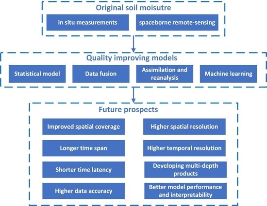
2. Models to Improve the Quality of SM Products
2.1. Statistical Model
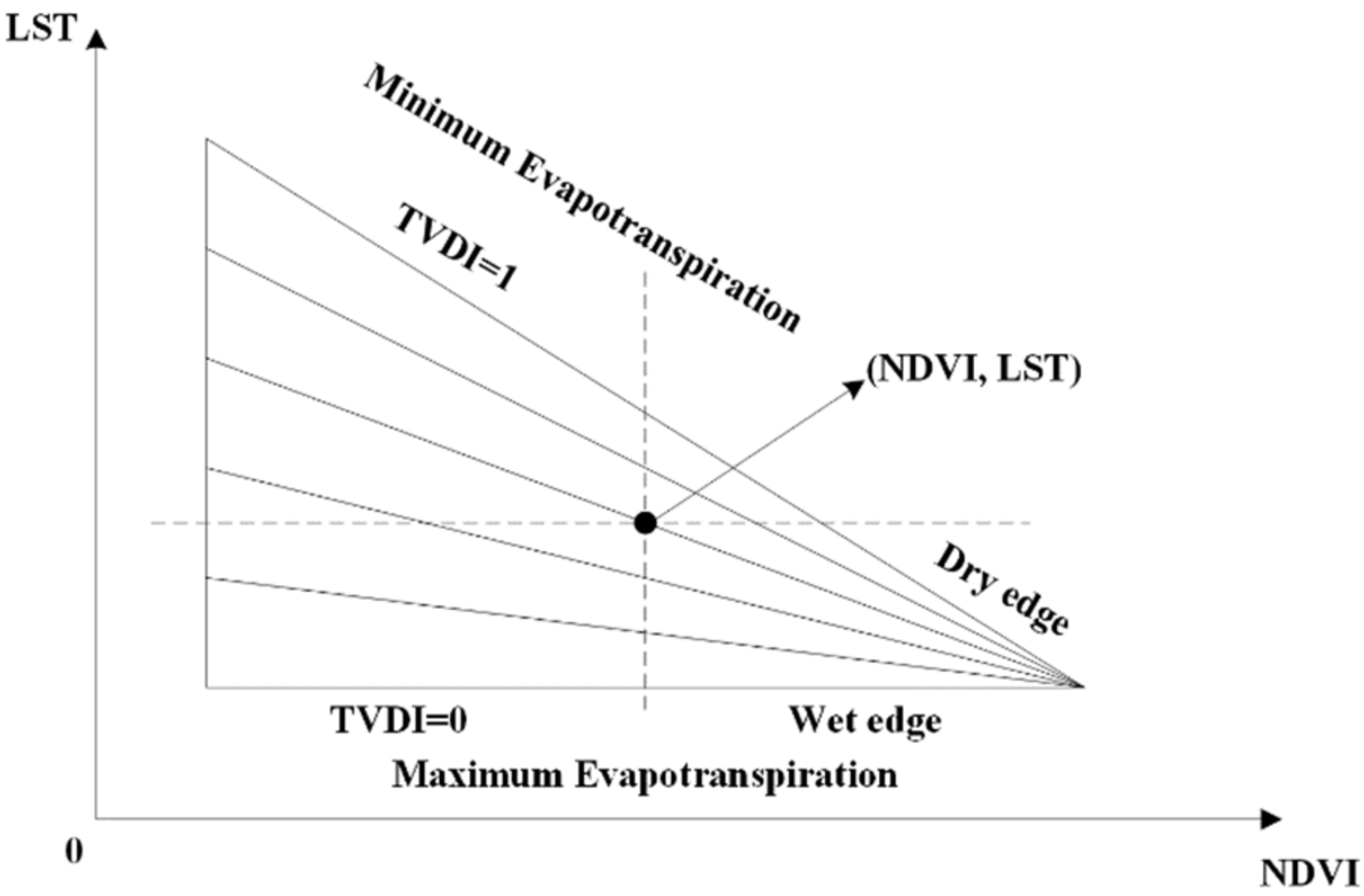
2.1.1. Triangular (Tri)-Based Method
2.1.2. Disaggregation Based on Physical and Theoretical Scale Change (DISPATCH) Algorithm
2.2. Data Fusion
- (1)
- ECV SM
- (2)
- SMOPS
- (3)
- SMAP
2.3. Assimilation and Reanalysis

| Type | Program | LSM | Assimilation Algorithm | Spatial Extent | Spatial Resolution | Time Range | Temporal Resolution | Publisher | Detailed Information |
|---|---|---|---|---|---|---|---|---|---|
| Assimilation | Global Land Data Assimilation System (GLDAS) | Mosaic, CLM, Noah | Ensemble Kalman filter, extended Kalman filter, optimal interpolation | global | 0.25° × 0.25°, 1° × 1° | 1948.1.1 ongoing | 3 h, 1 day, 1 month | NASA GSFC | [130] |
| North American Land Data Assimilation System (NLDAS) | Mosaic, CLM, Noah | Ensemble Kalman filter, extended Kalman filter, optimal interpolation | 67°W–125°W, 25°N–53°N | 0.125° × 0.125° | 1979.1.1 ongoing | 1 h, 1 month | NASA GSFC | [135,136] | |
| European Land Data Assimilation System (ELDAS) | Lokal Modell, ISBA and TERRA, TESSEL | Four-dimensional variational, Kalman filter, optimal interpolation | 15°W–38°E, 35°N–72°N | 0.2° × 0.2°, 1° × 1° | 1999.10–2000.12 | 3 h, 1 day | The European Centre for Medium-Range Weather Forecasts (ECMWF) | [137,138] | |
| CMA Land Data Assimilation System (CLDAS) | The Common Land Model, CLM, Noah | Three-dimensional variational, optimal interpolation | 60°E–160°E, 0–65°N | 0.0625° × 0.0625° | 2012.1.1 ongoing | 3 h, 1 day | CMA | [139,140] | |
| Satellite Application Facility on Support to Operational Hydrology and Water Management (H SAF) | The Hydrology Tiled ECMWF Scheme for Surface Exchanges over Land | Four-dimensional variational | Global | 1 km × 1 km; 12.5 km × 12.5 km; 25 km × 25 km; | 2005 ongoing | 1 day | European Organization for the Exploitation of Meteorological Satellites (EUMETSAT) | [26,141] | |
| Reanalysis | The National Centers for Environmental Prediction/the National Center for Atmospheric Research (NCEP/NCAR) | The T62/28-level NCEP global operational spectral model | Three-dimensional variational, four-dimensional variational, optimal interpolation, SSI | Global | 2.5° × 2.5° | 1948.1.1 ongoing | 6 h, 1 day, 1 month | The NOAA Earth System Research Laboratory Physical Sciences Laboratory | [142,143] |
| NCEP Climate Forecast System Reanalysis (CFSR) | NCEP Coupled Climate Forecast System Dynamical Model, the Seasonal Forecast Model | Three-dimensional variational, GSI | Global | 0.5° × 0.5°, 2.5° × 2.5° | 1979.1.1–2011.3.31 | 1 h, 6 h, 1 month | The NOAA National Centers for Environmental Information | [144] | |
| ECMWF Reanalysis v5 (ERA5) | Land-surface model (HTESSEL), ocean wave model | Four-dimensional variational | Global | 9 × 9 km2, 30 × 30 km2 | 1950.1 ongoing | 1 h, 1 day, 1 month | ECMWF | [145,146] | |
| Modern Era Retrospective-Analysis for Research and Applications (MERRA) | The GEOS-5 atmospheric general circulation model | Three-dimensional variational, Gridpoint Statistical Interpolation (GSI) | Global | 1/2° × 2/3°, 1.25° × 1.25°, 1° × 1.25° | 1979–2016.2 | 1 h, 3 h, 6 h | NASA GSFC | [147] | |
| the Japan Meteorological Agency (JMA) | MRI/NPD unified nonhydrostatic model | Four-dimensional variational | Global | 10 × 10 km2 | 1958–2013 | 6 h, 1 day | The Japan Meteorological Agency | [148] | |
| CMA Reanalysis (CRA) | Noah | EnKF, three-dimensional variational | Global | ~34 × 34 km2 | 1979–2018 | 6 h | CMA | [149,150] |
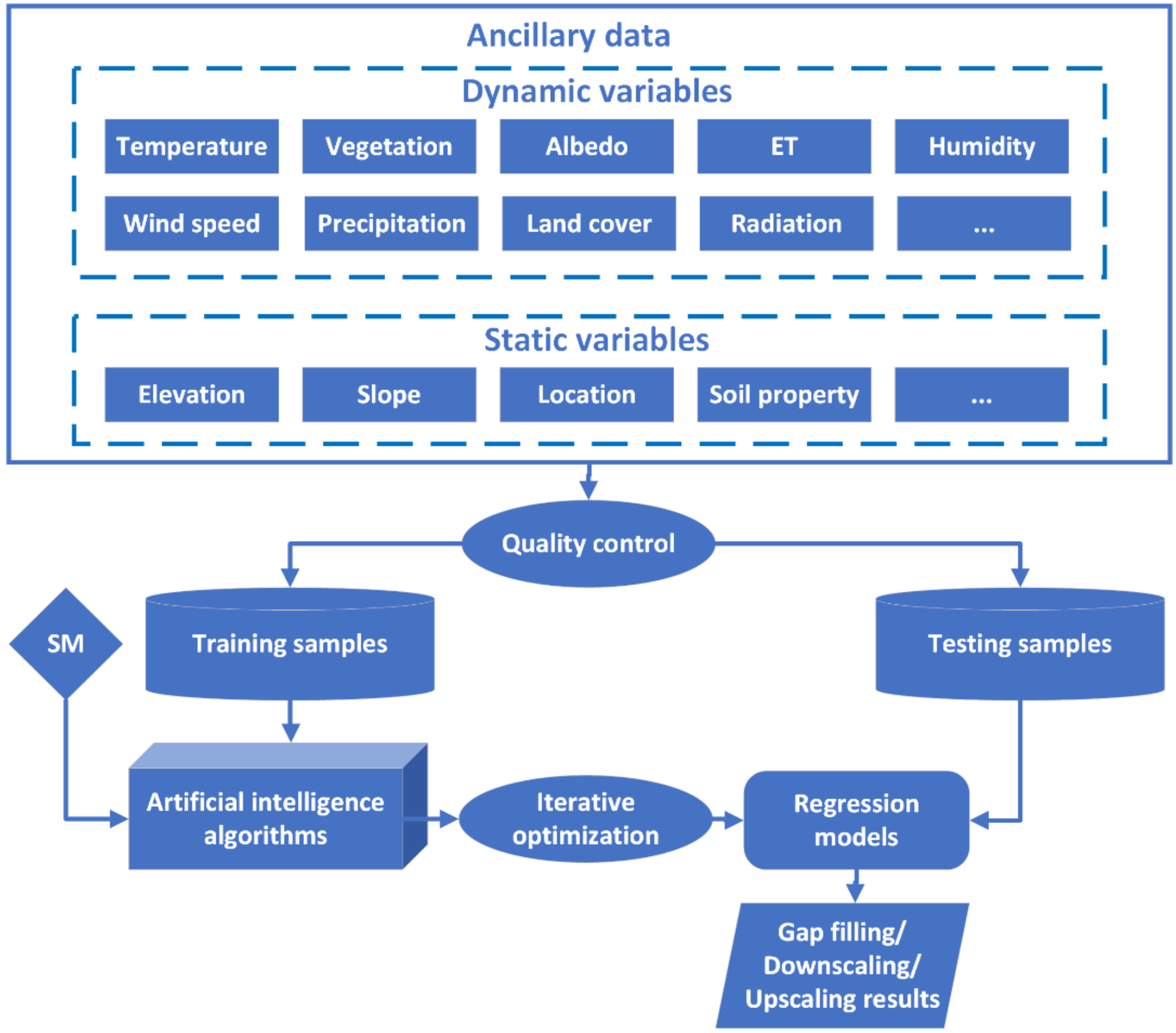
2.4. Machine Learning
2.4.1. Traditional Machine Learning
2.4.2. Deep Learning
| Type | Source | Algorithm | Target SM Data | Result | Conclusion |
|---|---|---|---|---|---|
| Gap filling | [170] | A two-layer machine learning-based framework | SMAP/Sentinel-1 SM product | 3 km resolution SM estimations at four study regions (Arkansas, Arizona, Iowa, and Oklahoma) in a 3.5-year period between 1 April 2015 and 30 September 2018 | The two-layer machine learning-based framework can reconstruct 3 km SM at gap regions with high fitting degree and low error |
| [171] | Long Short-Term Memory (LSTM) | SMAP passive SM product | 36 km resolution SM estimations in the continental United States from April 2015 to April 2017 | The LSTM exhibit good spatial and temporal generalization capability in simulating SM | |
| [152] | RF | ECV active-passive combined SM product | Global gap-filled monthly ECV SM from January 2001 to December 2012 | The gap-filled products achieve comparable performance as the original ECV | |
| [172] | Linear interpolation, cubic interpolation, SVM, and SVM combined with principal component analysis | ECV active-passive combined SM product | Gap-filled daily ECV SM in Southern Europe from 2003 to 2015 | There are no substantial differences between the accuracy of the original and the SVM-reconstructed SM products | |
| Downscaling | [153] | ANN, SVM, relevance vector machine, the generalized linear model | SMOS SM product | 0.05° resolution SM estimations in southwestern England from February 2011 to January 2012 | The ANN outperforms other algorithms in SM downscaling with higher accuracy |
| [173] | RF | ECV active-passive combined SM product, CLDAS SM retrievals at 0–10 cm depth, in situ measurements | 1 km resolution SM estimations at crop growth periods during 2015–2016 over Hebei Province, which is one of the major grain production regions of China | The RF model downscaled SM results display generally comparable and even better accuracy than the original SM products | |
| [14] | ANN, Bayesian, CART, KNN, RF, SVM | ECV active-passive combined SM product | 1 km resolution SM estimations at four case study regions with quite different climate types and underlying surfaces across the globe | The RF model downscaled SM achieves excellent performance with a high correlation coefficient and a low regression error | |
| [154] | CART, GBDT, RF, XGBoost | SMAP passive and enhanced passive SM products | 1 km resolution SM estimations in western Europe from January 2016 to December 2017 | Multi-decision tree-derived RF, XGBoost, and GBDT could all achieve good performances in SM downscaling, and GBDT shows slight superiority to the other two methods | |
| [9] | RF | ECV, SMAP, and CLDAS SM products, in situ measurements | 30 m resolution SM estimations during 1 March–31 October of years 2015, 2016, and 2017 in the Haihe Basin, which is one of the major grain production regions of China | The potential of the RF model is maximized to provide accurate and highly valuable SM estimations for hydrological research at the field scale | |
| [174] | H2O | AMSR-2 SM products, in situ measurements | 4 km resolution SM estimations in the Korean Peninsula from 2014 to 2016 | The H2O deep learning downscaled SM estimations indicate higher agreement with the in situ measurements than the original AMSR-2 and GLDAS SM products | |
| [175] | CNN, GRU | MODIS-based surface soil moisture data as a target variable obtained from the GLDAS 2.0 model | Forecasted SM in the Australian Murray Darling Basin on the 1st, 5th, 7th, 14th, 21st, and 30th day between 1 February 2003 and 31 March 2020 | The CNN-GRU hybrid models are considerably superior in SM forecasting to standalone methods | |
| Upscaling | [156] | XGBoost | Multi-layer in situ measurements (5, 10, 20, 50, and 100 cm depths), SMAP surface (0–5 cm), and root-zone (0–100 cm) SM products | 1 km resolution SM retrievals at 5, 10, 20, 50, and 100 cm depths over the United States from 31 March 2015 to 29 February 2019 | The multi-layer SM retrievals well match the temporal dynamics of SM; the ubRMSE is less than 0.04 m3/m3 at most sites |
| [176] | Bayesian | 0–5 cm depth in situ measurements | 100 km grid-box SM at 0–5 cm depth over the central Tibetan Plateau from 1 August 2010 to 20 September 2011 | The upscaled SM revealed higher reliability and robustness compared to the point-scale data | |
| [177] | RF | In situ measurements from three networks, respectively | Gridded SM estimations with an approximate spatial resolution of 100 m at three networks located in North America | The RF model upscaled SM expresses high level matching degree against field samples and outperforms other common regression methods. | |
| [178] | DFNN | Top 10 cm in situ measurements at croplands | 750 m resolution SM over the cropland of China on the 1st, 11th, and 21st day from May to October in 2012 to 2015 | The deep learning model retrieved SM shows better accuracy than SMAP radar and GLDAS SM products |
3. Applications
3.1. Drought Monitoring
3.2. Climate Change
3.3. Hydrology
3.4. Ecology
4. Outlook
4.1. Improved Spatial Coverage
4.2. Higher Spatial Resolution
4.3. Longer Time Span
4.4. Higher Temporal Resolution
4.5. Shorter Time Latency
4.6. Developing Multi-Depth Products
4.7. Higher Data Accuracy
4.8. Better Model Performance and Interpretability
5. Conclusions
Author Contributions
Funding
Data Availability Statement
Acknowledgments
Conflicts of Interest
Acronyms
| AMSR-2 | the Advanced Microwave Scanning Radiometer 2 |
| AMSR-E | the Advanced Microwave Scanning Radiometer for the Earth observing system |
| ANN | Artificial Neural Network |
| ASCAT MetOp-A | the Advanced Scatterometer on MetOp-A |
| ASCAT MetOp-B | the Advanced Scatterometer on MetOp-B |
| CART | Classification and Regression Trees |
| CFSR | the NCEP Climate Forecast System Reanalysis |
| CLDAS | the CMA Land Data Assimilation System |
| CMA | China Meteorological Administration |
| CRA | the CMA Reanalysis |
| CLM | the Community Land Model |
| CNN | Convolutional Neural Network |
| CYGNSS | Cyclone Global Navigation Satellite System |
| DEM | Digital Elevation Model |
| DBN | Deep Belief Network |
| DFNN | Deep Feedforward Neural Network |
| DISPATCH | Disaggregation based on physical and theoretical scale change |
| ECV SM | the Essential Climate Variable Soil Moisture |
| ECMWF | the European Centre for Medium-Range Weather Forecasts |
| ELDAS | the European Land Data Assimilation System |
| ENVISAT | the Environmental Satellite |
| ERA5 | the ECMWF Reanalysis v5 |
| ERS-1 | the European Remote-Sensing Satellite-1 |
| ERS-2 | the European Remote-Sensing Satellite-2 |
| ESA | the European Space Agency |
| ET | Evapotranspiration |
| EUMETSAT | European Organization for the Exploitation of Meteorological Satellites |
| EVI | enhanced vegetation index |
| FY-3B | FengYun-3B |
| FY-3C | FengYun-3C |
| GBDT | Gradient Boost Decision Tree |
| GLDAS | the Global Land Data Assimilation System |
| GPM GMI | the Global Precipitation Measurement Microwave Imager |
| GRU | Gated Recurrent Unit |
| GSFC | Goddard Space Flight Center |
| H SAF | Satellite Application Facility on Support to Operational Hydrology and Water Management |
| ISMN | the International Soil Moisture Network |
| JMA | the Japan Meteorological Agency |
| KNN | K Nearest Neighbor |
| LSM | the Land Surface Model |
| LST | land surface temperature |
| LSTM | Long Short Term Memory |
| MERRA | the Modern Era Retrospective-Analysis for Research and Applications |
| MODIS | the Moderate Resolution Imaging Spectroradiometer |
| NCEP/NCAR | the National Centers for Environmental Prediction/the National Center for Atmospheric Research |
| NDVI | Normalized Difference Vegetation Index |
| NLDAS | the North American Land Data Assimilation System |
| NPP | Net Primary Productivity |
| NSIDC | the National Snow and Ice Data Center |
| ResNet | Residual Network |
| RF | Random Forest |
| RFI | Radio Frequency Interference |
| SAR | Synthetic Aperture Radar |
| SAVI | Soil Adjusted Vegetation Index |
| SEE | the Soil Evaporative Efficiency |
| SM | Soil Moisture |
| SMMR | the Scanning Multichannel Microwave Radiometer |
| SMAP | the Soil Moisture Active Passive |
| SMOPS | the Soil Moisture Operational Product System |
| SMOS | the Soil Moisture and Ocean Salinity |
| SSM/I | the Special Sensor Microwave Imager |
| ST | Soil Temperature |
| SVM | Support Vector Machine |
| Tri | the Triangular-Based Method |
| TRMM TMI | the Tropical Rainfall Measuring Mission Microwave Imager |
| TVDI | Temperature Vegetation Drought Index |
| UTC | Coordinated Universal Time |
| XGB | Extreme Gradient Boost |
References
- Babaeian, E.; Sadeghi, M.; Jones, S.B.; Montzka, C.; Vereecken, H.; Tuller, M. Ground, proximal, and satellite remote sensing of soil moisture. Rev. Geophys. 2019, 57, 530–616. [Google Scholar] [CrossRef] [Green Version]
- Li, Z.-L.; Leng, P.; Zhou, C.; Chen, K.-S.; Zhou, F.-C.; Shang, G.-F. Soil moisture retrieval from remote sensing measurements: Current knowledge and directions for the future. Earth-Sci. Rev. 2021, 218, 103673. [Google Scholar] [CrossRef]
- Baatz, R.; Hendricks Franssen, H.; Euskirchen, E.; Sihi, D.; Dietze, M.; Ciavatta, S.; Fennel, K.; Beck, H.; De Lannoy, G.; Pauwels, V. Reanalysis in Earth system science: Toward terrestrial ecosystem reanalysis. Rev. Geophys. 2021, 59, e2020RG000715. [Google Scholar] [CrossRef]
- Kornelsen, K.C.; Coulibaly, P. Advances in soil moisture retrieval from synthetic aperture radar and hydrological applications. J. Hydrol. 2013, 476, 460–489. [Google Scholar] [CrossRef]
- Gruber, A.; Dorigo, W.A.; Zwieback, S.; Xaver, A.; Wagner, W. Characterizing Coarse-Scale Representativeness of in situ Soil Moisture Measurements from the International Soil Moisture Network. Vadose Zone J. 2013, 12, 522–525. [Google Scholar] [CrossRef] [Green Version]
- Wang, L.; Qu, J.J. Satellite remote sensing applications for surface soil moisture monitoring: A review. Front. Earth Sci. China 2009, 3, 237–247. [Google Scholar] [CrossRef]
- Ali, I.; Greifeneder, F.; Stamenkovic, J.; Neumann, M.; Notarnicola, C. Review of Machine Learning Approaches for Biomass and Soil Moisture Retrievals from Remote Sensing Data. Remote Sens. 2015, 7, 221–236. [Google Scholar] [CrossRef] [Green Version]
- Li, Y.; Shu, H.; Mousa, B.; Jiao, Z. Novel Soil Moisture Estimates Combining the Ensemble Kalman Filter Data Assimilation and the Method of Breeding Growing Modes. Remote Sens. 2020, 12, 889. [Google Scholar] [CrossRef] [Green Version]
- Abowarda, A.S.; Bai, L.; Zhang, C.; Long, D.; Li, X.; Huang, Q.; Sun, Z. Generating surface soil moisture at 30 m spatial resolution using both data fusion and machine learning toward better water resources management at the field scale. Remote Sens. Environ. 2021, 255, 112301. [Google Scholar] [CrossRef]
- Llamas, R.; Guevara, M.; Rorabaugh, D.; Taufer, M.; Vargas, R. Spatial Gap-Filling of ESA CCI Satellite-Derived Soil Moisture Based on Geostatistical Techniques and Multiple Regression. Remote Sens. 2020, 12, 665. [Google Scholar] [CrossRef] [Green Version]
- Sadeghi, M.; Babaeian, E.; Tuller, M.; Jones, S. The optical trapezoid model: A novel approach to remote sensing of soil moisture applied to Sentinel-2 and Landsat-8 observations. Remote Sens. Environ. 2017, 198, 52–68. [Google Scholar] [CrossRef] [Green Version]
- Babaeian, E.; Sadeghi, M.; Franz, T.E.; Jones, S.; Tuller, M. Mapping soil moisture with the OPtical TRApezoid Model (OPTRAM) based on long-term MODIS observations. Remote Sens. Environ. 2018, 211, 425–440. [Google Scholar] [CrossRef]
- Leng, P.; Song, X.; Duan, S.-B.; Li, Z.-L. A practical algorithm for estimating surface soil moisture using combined optical and thermal infrared data. Int. J. Appl. Earth Obs. Geoinf. 2016, 52, 338–348. [Google Scholar] [CrossRef]
- Liu, Y.; Jing, W.; Wang, Q.; Xia, X. Generating high-resolution daily soil moisture by using spatial downscaling techniques: A comparison of six machine learning algorithms. Adv. Water Resour. 2020, 141, 103601. [Google Scholar] [CrossRef]
- Walker, J.P.; Houser, P.R. A methodology for initializing soil moisture in a global climate model: Assimilation of near-surface soil moisture observations. J. Geophys. Res. Atmos. 2001, 106, 11761–11774. [Google Scholar] [CrossRef] [Green Version]
- Sheffield, J.; Wood, E.F. Global Trends and Variability in Soil Moisture and Drought Characteristics, 1950–2000, from Observation-Driven Simulations of the Terrestrial Hydrologic Cycle. J. Clim. 2006, 21, 432–458. [Google Scholar] [CrossRef] [Green Version]
- Peng, J.; Loew, A.; Merlin, O.; Verhoest, N.E.C. A review of spatial downscaling of satellite remotely sensed soil moisture. Rev. Geophys. 2017, 55, 341–366. [Google Scholar] [CrossRef]
- Dorigo, W.A.; Wagner, W.; Hohensinn, R.; Hahn, S.; Paulik, C.; Xaver, A.; Gruber, A.; Drusch, M.; Mecklenburg, S.; Oevelen, P.V. The International Soil Moisture Network: A data hosting facility for global in situ soil moisture measurements. Hydrol. Earth Syst. Sci. 2011, 15, 1675–1698. [Google Scholar] [CrossRef] [Green Version]
- Dorigo, W.A.; Xaver, A.; Vreugdenhil, M.; Gruber, A.; Hegyiová, A.; Sanchis-Dufau, A.D.; Zamojski, D.; Cordes, C.; Wagner, W.; Drusch, M. Global Automated Quality Control of In Situ Soil Moisture Data from the International Soil Moisture Network. Vadose Zone J. 2013, 12, 918–924. [Google Scholar] [CrossRef]
- Paulik, C.; Dorigo, W.; Wagner, W.; Kidd, R. Validation of the ASCAT Soil Water Index using in situ data from the International Soil Moisture Network. Int. J. Appl. Earth Obs. Geoinf. 2014, 30, 1–8. [Google Scholar] [CrossRef]
- Chen, Y.; Yang, K.; Qin, J.; Cui, Q.; Lu, H.; Zhu, L.; Han, M.; Tang, W. Evaluation of SMAP, SMOS, and AMSR2 soil moisture retrievals against observations from two networks on the Tibetan Plateau. J. Geophys. Res. Atmos. 2017, 122, 5780–5792. [Google Scholar] [CrossRef]
- Ma, H.; Zeng, J.; Chen, N.; Zhang, X.; Cosh, M.H.; Wang, W. Satellite surface soil moisture from SMAP, SMOS, AMSR2 and ESA CCI: A comprehensive assessment using global ground-based observations. Remote Sens. Environ. 2019, 231, 111215. [Google Scholar] [CrossRef]
- Griesfeller, A.; Lahoz, W.A.; De Jeu, R.A.M.; Dorigo, W.; Haugen, L.E.; Svendby, T.M.; Wagner, W. Evaluation of satellite soil moisture products over Norway using ground-based observations. Int. J. Appl. Earth Obs. Geoinf. 2016, 45, 155–164. [Google Scholar] [CrossRef] [Green Version]
- Dorigo, W.A.; Gruber, A.; Jeu, R.A.M.D.; Wagner, W.; Stacke, T.; Loew, A.; Albergel, C.; Brocca, L.; Chung, D.; Parinussa, R.M. Evaluation of the ESA CCI soil moisture product using ground-based observations. Remote Sens. Environ. 2015, 162, 380–395. [Google Scholar] [CrossRef]
- Beck, H.E.; Pan, M.; Miralles, D.G.; Reichle, R.H.; Dorigo, W.A.; Hahn, S.; Sheffield, J.; Karthikeyan, L.; Balsamo, G.; Parinussa, R.M. Evaluation of 18 satellite-and model-based soil moisture products using in situ measurements from 826 sensors. Hydrol. Earth Syst. Sci. 2021, 25, 17–40. [Google Scholar] [CrossRef]
- Albergel, C.; De Rosnay, P.; Gruhier, C.; Muñoz-Sabater, J.; Hasenauer, S.; Isaksen, L.; Kerr, Y.; Wagner, W. Evaluation of remotely sensed and modelled soil moisture products using global ground-based in situ observations. Remote Sens. Environ. 2012, 118, 215–226. [Google Scholar] [CrossRef]
- Chen, S.; Liu, Y.; Wen, Z. Satellite retrieval of soil moisture: An overview. Adv. Earth Sci. 2012, 27, 1192–1203. [Google Scholar]
- Goward, S.N.; Xue, Y.; Czajkowski, K.P. Evaluating land surface moisture conditions from the remotely sensed temperature/vegetation index measurements: An exploration with the simplified simple biosphere model. Remote Sens. Environ. 2002, 79, 225–242. [Google Scholar] [CrossRef]
- Quiring, S.M.; Ganesh, S. Evaluating the utility of the Vegetation Condition Index (VCI) for monitoring meteorological drought in Texas. Agric. For. Meteorol. 2010, 150, 330–339. [Google Scholar] [CrossRef]
- Gu, Y.; Hunt, E.; Wardlow, B.; Basara, J.B.; Brown, J.F.; Verdin, J.P. Evaluation of MODIS NDVI and NDWI for vegetation drought monitoring using Oklahoma Mesonet soil moisture data. Geophys. Res. Lett. 2008, 35, 1092–1104. [Google Scholar] [CrossRef] [Green Version]
- Patel, N.; Anapashsha, R.; Kumar, S.; Saha, S.; Dadhwal, V. Assessing potential of MODIS derived temperature/vegetation condition index (TVDI) to infer soil moisture status. Int. J. Remote Sens. 2009, 30, 23–39. [Google Scholar] [CrossRef]
- Mallick, K.; Bhattacharya, B.K.; Patel, N. Estimating volumetric surface moisture content for cropped soils using a soil wetness index based on surface temperature and NDVI. Agric. For. Meteorol. 2009, 149, 1327–1342. [Google Scholar] [CrossRef]
- Walker, J.P.; Houser, P.R.; Willgoose, G.R. Active microwave remote sensing for soil moisture measurement: A field evaluation using ERS-2. Hydrol. Processes 2004, 18, 1975–1997. [Google Scholar] [CrossRef]
- Barrett, B.W.; Dwyer, E.; Whelan, P. Soil moisture retrieval from active spaceborne microwave observations: An evaluation of current techniques. Remote Sens. 2009, 1, 210–242. [Google Scholar] [CrossRef] [Green Version]
- Wagner, W.; Dorigo, W.; de Jeu, R.; Fernandez, D.; Benveniste, J.; Haas, E.; Ertl, M. Fusion of Active and Passive Microwave Observations to Create AN Essential Climate Variable Data Record on Soil Moisture. ISPRS Ann. Photogramm. Remote Sens. Spatial Inf. Sci. 2012, I-7, 315–321. [Google Scholar] [CrossRef]
- Zhao, W.; Li, A.; Jin, H.; Zhang, Z.; Bian, J.; Yin, G. Performance evaluation of the triangle-based empirical soil moisture relationship models based on Landsat-5 TM data and in situ measurements. IEEE Trans. Geosci. Remote Sens. 2017, 55, 2632–2645. [Google Scholar] [CrossRef]
- Carlson, T.N.; Perry, E.M.; Schmugge, T.J. Remote estimation of soil moisture availability and fractional vegetation cover for agricultural fields. Agric. For. Meteorol. 1990, 52, 45–69. [Google Scholar] [CrossRef]
- Magagi, R.D.; Kerr, Y.H. Retrieval of soil moisture and vegetation characteristics by use of ERS-1 wind scatterometer over arid and semi-arid areas. J. Hydrol. 1997, 188–189, 361–384. [Google Scholar] [CrossRef]
- Altese, E.; Bolognani, O.; Mancini, M.; Troch, P.A. Retrieving soil moisture over bare soil from ERS 1 synthetic aperture radar data: Sensitivity analysis based on a theoretical surface scattering model and field data. Water Resour. Res. 1996, 32, 653–661. [Google Scholar] [CrossRef]
- Wang, C.; Qi, J.; Moran, S.; Marsett, R. Soil moisture estimation in a semiarid rangeland using ERS-2 and TM imagery. Remote Sens. Environ. 2004, 90, 178–189. [Google Scholar] [CrossRef]
- Pathe, C.; Wagner, W.; Sabel, D.; Doubkova, M.; Basara, J.B. Using ENVISAT ASAR global mode data for surface soil moisture retrieval over Oklahoma, USA. IEEE Trans. Geosci. Remote Sens. 2009, 47, 468–480. [Google Scholar] [CrossRef]
- Bartalis, Z.; Wagner, W.; Naeimi, V.; Hasenauer, S.; Scipal, K.; Bonekamp, H.; Figa, J.; Anderson, C. Initial soil moisture retrievals from the METOP-A Advanced Scatterometer (ASCAT). Geophys. Res. Lett. 2007, 34. [Google Scholar] [CrossRef] [Green Version]
- Gruber, A.; Paloscia, S.; Santi, E.; Notarnicola, C.; Pasolli, L.; Smolander, T.; Pulliainen, J.; Mittelbach, H.; Dorigo, W.; Wagner, W. Performance inter-comparison of soil moisture retrieval models for the MetOp-A ASCAT instrument. In Proceedings of the 2014 IEEE Geoscience and Remote Sensing Symposium, Quebec City, QC, Canada, 13–18 July 2014; pp. 2455–2458. [Google Scholar]
- Brocca, L.; Crow, W.T.; Ciabatta, L.; Massari, C.; De Rosnay, P.; Enenkel, M.; Hahn, S.; Amarnath, G.; Camici, S.; Tarpanelli, A. A review of the applications of ASCAT soil moisture products. IEEE J. Sel. Top. Appl. Earth Obs. Remote Sens. 2017, 10, 2285–2306. [Google Scholar] [CrossRef]
- Chew, C.; Small, E. Description of the UCAR/CU soil moisture product. Remote Sens. 2020, 12, 1558. [Google Scholar] [CrossRef]
- Aubert, M.; Baghdadi, N.; Zribi, M.; Douaoui, A.; Loumagne, C.; Baup, F.; El Hajj, M.; Garrigues, S. Analysis of TerraSAR-X data sensitivity to bare soil moisture, roughness, composition and soil crust. Remote Sens. Environ. 2011, 115, 1801–1810. [Google Scholar] [CrossRef] [Green Version]
- Kseneman, M.; Gleich, D.; Potočnik, B. Soil-moisture estimation from TerraSAR-X data using neural networks. Mach. Vis. Appl. 2012, 23, 937–952. [Google Scholar] [CrossRef]
- Baghdadi, N.; Aubert, M.; Zribi, M. Use of TerraSAR-X Data to Retrieve Soil Moisture Over Bare Soil Agricultural Fields. IEEE Geosci. Remote Sens. Lett. 2012, 9, 512–516. [Google Scholar] [CrossRef] [Green Version]
- Balenzano, A.; Mattia, F.; Satalino, G.; Lovergine, F.P.; Palmisano, D.; Peng, J.; Marzahn, P.; Wegmüller, U.; Cartus, O.; Dąbrowska-Zielińska, K.; et al. Sentinel-1 soil moisture at 1 km resolution: A validation study. Remote Sens. Environ. 2021, 263, 112554. [Google Scholar] [CrossRef]
- Balenzano, A.; Mattia, F.; Satalino, G.; Lovergine, F.P.; Palmisano, D.; Davidson, M.W.J. Dataset of Sentinel-1 surface soil moisture time series at 1 km resolution over Southern Italy. Data Brief 2021, 38, 107345. [Google Scholar] [CrossRef]
- Owe, M.; de Jeu, R.; Holmes, T. Multisensor historical climatology of satellite-derived global land surface moisture. J. Geophys. Res. Earth Surf. 2008, 113. [Google Scholar] [CrossRef]
- Reichle, R.H.; Koster, R.D.; Liu, P.; Mahanama, S.P.; Njoku, E.G.; Owe, M. Comparison and assimilation of global soil moisture retrievals from the Advanced Microwave Scanning Radiometer for the Earth Observing System (AMSR-E) and the Scanning Multichannel Microwave Radiometer (SMMR). J. Geophys. Res. Atmos. 2007, 112. [Google Scholar] [CrossRef]
- Ridder, K.D. Surface soil moisture monitoring over Europe using Special Sensor Microwave/Imager (SSM/I) imagery. J. Geophys. Res. 2003, 108, 4422. [Google Scholar] [CrossRef]
- Drusch, M.; Wood, E.F.; Gao, H. Observation operators for the direct assimilation of TRMM microwave imager retrieved soil moisture. Geophys. Res. Lett. 2005, 32. [Google Scholar] [CrossRef]
- Njoku, E.G.; Jackson, T.J.; Lakshmi, V.; Chan, T.K.; Nghiem, S.V. Soil moisture retrieval from AMSR-E. IEEE Trans. Geosci. Remote Sens. 2003, 41, 215–229. [Google Scholar] [CrossRef]
- Brocca, L.; Hasenauer, S.; Lacava, T.; Melone, F.; Moramarco, T.; Wagner, W.; Dorigo, W.; Matgen, P.; Martínez-Fernández, J.; Llorens, P. Soil moisture estimation through ASCAT and AMSR-E sensors: An intercomparison and validation study across Europe. Remote Sens. Environ. 2011, 115, 3390–3408. [Google Scholar] [CrossRef]
- Bindlish, R.; Cosh, M.H.; Jackson, T.J.; Koike, T.; Fujii, H.; Chan, S.K.; Asanuma, J.; Berg, A.; Bosch, D.D.; Caldwell, T. GCOM-W AMSR2 Soil Moisture Product Validation Using Core Validation Sites. IEEE J. Sel. Top. Appl. Earth Obs. Remote Sens. 2018, 11, 209–219. [Google Scholar] [CrossRef] [Green Version]
- Parinussa, R.M.; Holmes, T.R.H.; Wanders, N.; Dorigo, W.A.; De Jeu, R.A.M. A Preliminary Study toward Consistent Soil Moisture from AMSR2. J. Hydrometeorol. 2013, 16, 932–947. [Google Scholar] [CrossRef]
- Li, L.; Gaiser, P.W.; Gao, B.C.; Bevilacqua, R.M.; Jackson, T.J.; Njoku, E.G.; Rudiger, C.; Calvet, J.C.; Bindlish, R. WindSat Global Soil Moisture Retrieval and Validation. IEEE Trans. Geosci. Remote Sens. 2010, 48, 2224–2241. [Google Scholar] [CrossRef]
- Gaiser, P.W.; St Germain, K.M.; Twarog, E.M.; Poe, G.A.; Purdy, W.; Richardson, D.; Grossman, W.; Jones, W.L.; Spencer, D.; Golba, G. The WindSat spaceborne polarimetric microwave radiometer: Sensor description and early orbit performance. IEEE Trans. Geosci. Remote Sens. 2004, 42, 2347–2361. [Google Scholar] [CrossRef]
- Al Bitar, A.; Leroux, D.; Kerr, Y.H.; Merlin, O.; Richaume, P.; Sahoo, A.; Wood, E.F. Evaluation of SMOS soil moisture products over continental US using the SCAN/SNOTEL network. IEEE Trans. Geosci. Remote Sens. 2012, 50, 1572–1586. [Google Scholar] [CrossRef] [Green Version]
- Liu, Y.; Zhou, Y.; Lu, N.; Tang, R.; Liu, N.; Li, Y.; Yang, J.; Jing, W.; Zhou, C. Comprehensive assessment of Fengyun-3 satellites derived soil moisture with in-situ measurements across the globe. J. Hydrol. 2021, 594, 125949. [Google Scholar] [CrossRef]
- Parinussa, R.M.; Wang, G.; Holmes, T.R.H.; Liu, Y.Y.; Dolman, A.J.; Jeu, R.A.M.D.; Jiang, T.; Zhang, P.; Shi, J. Global surface soil moisture from the Microwave Radiation Imager onboard the Fengyun-3B satellite. Int. J. Remote Sens. 2014, 35, 7007–7029. [Google Scholar] [CrossRef]
- Wu, S.; Chen, J. Instrument Performance and Cross Calibration of FY-3C MWRI. In Proceedings of the 2016 IEEE International Geoscience and Remote Sensing Symposium (IGARSS), Beijing, China, 10–15 July 2016; pp. 388–391. [Google Scholar]
- Zhang, S.; Weng, F.; Yao, W. A Multivariable Approach for Estimating Soil Moisture from Microwave Radiation Imager (MWRI). J. Meteorol. Res. 2020, 34, 732–747. [Google Scholar] [CrossRef]
- Entekhabi, D.; Njoku, E.G.; O’Neill, P.E.; Kellogg, K.H.; Crow, W.T.; Edelstein, W.N.; Entin, J.K.; Goodman, S.D.; Jackson, T.J.; Johnson, J.; et al. The Soil Moisture Active Passive (SMAP) Mission. Proc. IEEE 2010, 98, 704–716. [Google Scholar] [CrossRef]
- Chan, S.K.; Bindlish, R.; O’Neill, P.E.; Njoku, E.; Jackson, T.; Colliander, A.; Fan, C.; Burgin, M.; Dunbar, S.; Piepmeier, J. Assessment of the SMAP Passive Soil Moisture Product. IEEE Trans. Geosci. Remote Sens. 2016, 54, 4994–5007. [Google Scholar] [CrossRef]
- Piepmeier, J.R.; Johnson, J.T.; Mohammed, P.N.; Bradley, D.; Ruf, C.; Aksoy, M.; Garcia, R.; Hudson, D.; Miles, L.; Wong, M. Radio-Frequency Interference Mitigation for the Soil Moisture Active Passive Microwave Radiometer. IEEE Trans. Geosci. Remote Sens. 2014, 52, 761–775. [Google Scholar] [CrossRef]
- Lacava, T.; Faruolo, M.; Pergola, N.; Coviello, I.; Tramutoli, V. A comprehensive analysis of AMSRE C- and X-bands Radio Frequency Interferences. In Proceedings of the Microwave Radiometry and Remote Sensing of the Environment, Rome, Italy, 5–9 March 2012; pp. 1–4. [Google Scholar]
- Draper, D.W. Radio Frequency Environment for Earth-Observing Passive Microwave Imagers. IEEE J. Sel. Top. Appl. Earth Obs. Remote Sens. 2018, 11, 1913–1922. [Google Scholar] [CrossRef]
- Zou, X.; Zhao, J.; Weng, F.; Qin, Z. Detection of Radio-Frequency Interference Signal Over Land From FY-3B Microwave Radiation Imager (MWRI). Adv. Meteorol. Sci. Technol. 2013, 50, 4994–5003. [Google Scholar] [CrossRef]
- Liu, Y.; Yao, L.; Jing, W.; Di, L.; Yang, J.; Li, Y. Comparison of two satellite-based soil moisture reconstruction algorithms: A case study in the state of Oklahoma, USA. J. Hydrol. 2020, 590, 125406. [Google Scholar] [CrossRef]
- Mohseni, F.; Mokhtarzade, M. A new soil moisture index driven from an adapted long-term temperature-vegetation scatter plot using MODIS data. J. Hydrol. 2020, 581, 124420. [Google Scholar] [CrossRef]
- Yang, J.; Zhang, D. Soil moisture estimation with a remotely sensed dry edge determination based on the land surface temperature-vegetation index method. J. Appl. Remote Sens. 2019, 13, 024511. [Google Scholar] [CrossRef]
- Peng, J.; Loew, A.; Zhang, S.; Wang, J.; Niesel, J. Spatial downscaling of satellite soil moisture data using a vegetation temperature condition index. IEEE Trans. Geosci. Remote Sens. 2016, 54, 558–566. [Google Scholar] [CrossRef]
- Holzman, M.; Rivas, R.; Piccolo, M. Geoinformation. Estimating soil moisture and the relationship with crop yield using surface temperature and vegetation index. Int. J. Appl. Earth Obs. Geoinf. 2014, 28, 181–192. [Google Scholar]
- Chen, J.; Wang, C.; Jiang, H.; Mao, L.; Yu, Z. Estimating soil moisture using Temperature–Vegetation Dryness Index (TVDI) in the Huang-huai-hai (HHH) plain. Int. J. Remote Sens. 2011, 32, 1165–1177. [Google Scholar] [CrossRef]
- Yuan, L.; Li, L.; Zhang, T.; Chen, L.; Zhao, J.; Hu, S.; Cheng, L.; Liu, W. Soil moisture estimation for the Chinese Loess Plateau using MODIS-derived ATI and TVDI. Remote Sens. 2020, 12, 3040. [Google Scholar] [CrossRef]
- Sandholt, I.; Rasmussen, K.; Andersen, J. A simple interpretation of the surface temperature/vegetation index space for assessment of surface moisture status. Remote Sens. Environ. 2002, 79, 213–224. [Google Scholar] [CrossRef]
- Carlson, T. An Overview of the Triangle Method for Estimating Surface Evapotranspiration and Soil Moisture from Satellite Imagery. Sensors 2007, 7, 1612–1629. [Google Scholar] [CrossRef] [Green Version]
- Rahmati, M.; Oskouei, M.M.; Neyshabouri, M.R.; Walker, J.P.; Fakherifard, A.; Ahmadi, A.; Mousavi, S.B. Soil moisture derivation using triangle method in the lighvan watershed, north western Iran. J. Soil Sci. Plant Nutr. 2015, 15, 167–178. [Google Scholar] [CrossRef]
- Tang, R.; Li, Z.-L.; Tang, B. An application of the Ts–VI triangle method with enhanced edges determination for evapotranspiration estimation from MODIS data in arid and semi-arid regions: Implementation and validation. Remote Sens. Environ. 2010, 114, 540–551. [Google Scholar] [CrossRef]
- Zhang, F.; Zhang, L.W.; Shi, J.J.; Huang, J.F. Soil Moisture Monitoring Based on Land Surface Temperature-Vegetation Index Space Derived from MODIS Data. Pedosphere 2014, 24, 450–460. [Google Scholar] [CrossRef]
- Shafian, S.; Maas, S.J. Index of soil moisture using raw Landsat image digital count data in Texas high plains. Remote Sens. 2015, 7, 2352–2372. [Google Scholar] [CrossRef] [Green Version]
- Sun, H. Two-Stage Trapezoid: A New Interpretation of the Land Surface Temperature and Fractional Vegetation Coverage Space. IEEE J. Sel. Top. Appl. Earth Obs. Remote Sens. 2016, 9, 336–346. [Google Scholar] [CrossRef]
- Merlin, O.; Malbéteau, Y.; Notfi, Y.; Bacon, S.; Er-Raki, S.; Khabba, S.; Jarlan, L. Performance metrics for soil moisture downscaling methods: Application to DISPATCH data in central Morocco. Remote Sens. 2015, 7, 3783–3807. [Google Scholar] [CrossRef] [Green Version]
- Djamai, N.; Magagi, R.; Goïta, K.; Merlin, O.; Kerr, Y.; Roy, A. A combination of DISPATCH downscaling algorithm with CLASS land surface scheme for soil moisture estimation at fine scale during cloudy days. Remote Sens. Environ. 2016, 184, 1–14. [Google Scholar] [CrossRef]
- Fontanet, M.; Fernàndez-Garcia, D.; Ferrer, F. The value of satellite remote sensing soil moisture data and the DISPATCH algorithm in irrigation fields. Hydrol. Earth Syst. Sci. 2018, 22, 5889–5900. [Google Scholar] [CrossRef] [Green Version]
- Dumedah, G.; Walker, J.P.; Merlin, O. Root-zone soil moisture estimation from assimilation of downscaled Soil Moisture and Ocean Salinity data. Adv. Water Resour. 2015, 84, 14–22. [Google Scholar] [CrossRef]
- Malbéteau, Y.; Merlin, O.; Balsamo, G.; Er-Raki, S.; Khabba, S.; Walker, J.; Jarlan, L. Toward a surface soil moisture product at high spatiotemporal resolution: Temporally interpolated, spatially disaggregated SMOS data. J. Hydrometeorol. 2018, 19, 183–200. [Google Scholar] [CrossRef]
- Ojha, N.; Merlin, O.; Suere, C.; Escorihuela, M.J. Extending the Spatio-Temporal Applicability of DISPATCH Soil Moisture Downscaling Algorithm: A Study Case Using SMAP, MODIS and Sentinel-3 Data. Front. Environ. Sci. 2021, 9, 555216. [Google Scholar] [CrossRef]
- Merlin, O.; Chehbouni, A.G.; Kerr, Y.H.; Njoku, E.G.; Entekhabi, D. A combined modeling and multispectral/multiresolution remote sensing approach for disaggregation of surface soil moisture: Application to SMOS configuration. IEEE Trans. Geosci. Remote Sens. 2005, 43, 2036–2050. [Google Scholar] [CrossRef]
- Merlin, O.; Rudiger, C.; Bitar, A.A.; Richaume, P.; Walker, J.P.; Kerr, Y.H. Disaggregation of SMOS Soil Moisture in Southeastern Australia. IEEE Trans. Geosci. Remote Sens. 2012, 50, 1556–1571. [Google Scholar] [CrossRef] [Green Version]
- Merlin, O.; Escorihuela, M.J.; Mayoral, M.A.; Hagolle, O.; Al Bitar, A.; Kerr, Y. Self-calibrated evaporation-based disaggregation of SMOS soil moisture: An evaluation study at 3km and 100m resolution in Catalunya, Spain. Remote Sens. Environ. 2013, 130, 25–38. [Google Scholar] [CrossRef] [Green Version]
- Malbéteau, Y.; Merlin, O.; Molero, B.; Rüdiger, C.; Bacon, S. DisPATCh as a tool to evaluate coarse-scale remotely sensed soil moisture using localized in situ measurements: Application to SMOS and AMSR-E data in Southeastern Australia. Int. J. Appl. Earth Obs. Geoinf. 2016, 45, 221–234. [Google Scholar] [CrossRef]
- Dorigo, W.; Wagner, W.; Albergel, C.; Albrecht, F.; Balsamo, G.; Brocca, L.; Chung, D.; Ertl, M.; Forkel, M.; Gruber, A. ESA CCI Soil Moisture for improved Earth system understanding: State-of-the art and future directions. Remote Sens. Environ. 2017, 203, 185–215. [Google Scholar] [CrossRef]
- Naeimi, V.; Scipal, K.; Bartalis, Z.; Hasenauer, S.; Wagner, W. An improved soil moisture retrieval algorithm for ERS and METOP scatterometer observations. IEEE Trans. Geosci. Remote Sens. 2009, 47, 1999–2013. [Google Scholar] [CrossRef]
- De Jeu, R.A.M.; Holmes, T.R.H.; Panciera, R.; Walker, J.P. Parameterization of the Land Parameter Retrieval Model for L-Band Observations Using the NAFE’05 Data Set. IEEE Geosci. Remote Sens. Lett. 2009, 6, 630–634. [Google Scholar] [CrossRef]
- Gruber, A.; Scanlon, T.; van der Schalie, R.; Wagner, W.; Dorigo, W. Evolution of the ESA CCI Soil Moisture climate data records and their underlying merging methodology. Earth Syst. Sci. Data 2019, 11, 717–739. [Google Scholar] [CrossRef] [Green Version]
- Wang, S.; Mo, X.; Liu, S.; Lin, Z.; Hu, S. Validation and trend analysis of ECV soil moisture data on cropland in North China Plain during 1981–2010. Int. J. Appl. Earth Obs. Geoinf. 2016, 48, 110–121. [Google Scholar] [CrossRef]
- McNally, A.; Shukla, S.; Arsenault, K.R.; Wang, S.; Peters-Lidard, C.D.; Verdin, J.P. Evaluating ESA CCI soil moisture in East Africa. Int. J. Appl. Earth Obs. Geoinf. 2016, 48, 96–109. [Google Scholar] [CrossRef] [Green Version]
- Wang, Y.; Leng, P.; Peng, J.; Marzahn, P.; Ludwig, R. Global assessments of two blended microwave soil moisture products CCI and SMOPS with in-situ measurements and reanalysis data. Int. J. Appl. Earth Obs. Geoinf. 2021, 94, 102234. [Google Scholar] [CrossRef]
- González-Zamora, Á.; Sánchez, N.; Pablos, M.; Martínez-Fernández, J. CCI soil moisture assessment with SMOS soil moisture and in situ data under different environmental conditions and spatial scales in Spain. Remote Sens. Environ. 2018, 225, 469–482. [Google Scholar] [CrossRef]
- Liu, Y.; Yang, Y.; Yue, X. Evaluation of Satellite-Based Soil Moisture Products over Four Different Continental In-Situ Measurements. Remote Sens. 2018, 10, 1161. [Google Scholar] [CrossRef] [Green Version]
- Liu, J.; Zhan, X.; Hain, C.; Yin, J.; Fang, L.; Li, Z.; Zhao, L. NOAA Soil Moisture Operational Product System (SMOPS) and Its Validations. In Proceedings of the 2016 IEEE International Geoscience and Remote Sensing Symposium (IGARSS), Beijing, China, 10–15 July 2016; pp. 3477–3480. [Google Scholar]
- Jackson, T.J., III. Measuring surface soil moisture using passive microwave remote sensing. Hydrol. Processes 1993, 7, 139–152. [Google Scholar] [CrossRef]
- Yin, J.; Zhan, X.; Liu, J. NOAA Satellite Soil Moisture Operational Product System (SMOPS) Version 3.0 Generates Higher Accuracy Blended Satellite Soil Moisture. Remote Sens. 2020, 12, 2861. [Google Scholar] [CrossRef]
- Yin, J.; Zhan, X.; Liu, J.; Schull, M. An intercomparison of Noah model skills with benefits of assimilating SMOPS blended and individual soil moisture retrievals. Water Resour. Res. 2019, 55, 2572–2592. [Google Scholar] [CrossRef]
- Pan, M.; Cai, X.; Chaney, N.; Entekhabi, D.; Wood, E.F. An Initial Assessment of SMAP Soil Moisture Retrievals Using High Resolution Model Simulations and In-situ Observations: SMAP Comparisons. Geophys. Res. Lett. 2016, 43, 9662–9668. [Google Scholar] [CrossRef] [Green Version]
- Jagdhuber, T.; Entekhabi, D.; Das, N.N.; Link, M.; Baur, M.; Akbar, R.; Montzka, C.; Kim, S.; Yueh, S.; Baris, I. Physics-based modeling of active-passive microwave covariations for geophysical retrievals. In Proceedings of the IGARSS 2018–2018 IEEE International Geoscience and Remote Sensing Symposium, Valencia, Spain, 22–27 July 2018; pp. 250–253. [Google Scholar]
- Mo, T.; Choudhury, B.; Schmugge, T.; Wang, J.R.; Jackson, T. A model for microwave emission from vegetation-covered fields. J. Geophys. Res. Ocean. 1982, 87, 11229–11237. [Google Scholar] [CrossRef]
- Das, N.N.; Entekhabi, D.; Dunbar, R.S.; Chaubell, M.J.; Colliander, A.; Yueh, S.; Jagdhuber, T.; Chen, F.; Crow, W.; O’Neill, P.E. The SMAP and Copernicus Sentinel 1A/B microwave active-passive high resolution surface soil moisture product. Remote Sens. Environ. 2019, 233, 111380. [Google Scholar] [CrossRef]
- Kim, H.; Lee, S.; Cosh, M.H.; Lakshmi, V.; Kwon, Y.; McCarty, G.W. Assessment and Combination of SMAP and Sentinel-1A/B-Derived Soil Moisture Estimates With Land Surface Model Outputs in the Mid-Atlantic Coastal Plain, USA. IEEE Trans. Geosci. Remote Sens. 2020, 59, 991–1011. [Google Scholar] [CrossRef]
- Draper, C.; Reichle, R.; De Lannoy, G.; Liu, Q. Assimilation of passive and active microwave soil moisture retrievals. Geophys. Res. Lett. 2012, 39. [Google Scholar] [CrossRef] [Green Version]
- Bi, H.; Ma, J.; Zheng, W.; Zeng, J. Comparison of soil moisture in GLDAS model simulations and in situ observations over the Tibetan Plateau. J. Geophys. Res. Atmos. 2016, 121, 2658–2678. [Google Scholar] [CrossRef] [Green Version]
- Kumar, S.V.; Reichle, R.H.; Koster, R.D.; Crow, W.T.; Peters-Lidard, C.D. Role of subsurface physics in the assimilation of surface soil moisture observations. J. Hydrometeorol. 2009, 10, 1534–1547. [Google Scholar] [CrossRef]
- Weisse, A.; Michel, C.; Aubert, D.; Loumagne, C. Assimilation of Soil Moisture in a Hydrological Model for Flood Forecasting; IAHS Publication: Maastricht, The Netherlands, 2001; pp. 249–256. [Google Scholar]
- Bouttier, F.; Mahfouf, J.; Noilhan, J. Sequential assimilation of soil moisture from atmospheric low-level parameters. Part I: Sensitivity and calibration studies. J. Appl. Meteorol. Climatol. 1993, 32, 1335–1351. [Google Scholar] [CrossRef] [Green Version]
- Reichle, R.H.; Entekhabi, D.; McLaughlin, D.B. Downscaling of radio brightness measurements for soil moisture estimation: A four-dimensional variational data assimilation approach. Water Resour. Res. 2001, 37, 2353–2364. [Google Scholar] [CrossRef] [Green Version]
- De Rosnay, P.; Drusch, M.; Vasiljevic, D.; Balsamo, G.; Albergel, C.; Isaksen, L. A simplified extended Kalman filter for the global operational soil moisture analysis at ECMWF. Q. J. R. Meteorol. Soc. 2013, 139, 1199–1213. [Google Scholar] [CrossRef]
- Lan, X.; Guo, Z.; Tian, Y.; Lei, X.; Wang, J. Review in soil moisture remote sensing estimation based on data assimilation. Adv. Earth Sci. 2015, 30, 668–679. [Google Scholar]
- Montzka, C.; Moradkhani, H.; Weihermüller, L.; Franssen, H.-J.H.; Canty, M.; Vereecken, H. Hydraulic parameter estimation by remotely-sensed top soil moisture observations with the particle filter. J. Hydrol. 2011, 399, 410–421. [Google Scholar] [CrossRef]
- Huang, C.; Li, X.; Lu, L.; Gu, J. Experiments of one-dimensional soil moisture assimilation system based on ensemble Kalman filter. Remote Sens. Environ. 2008, 112, 888–900. [Google Scholar] [CrossRef]
- Brandhorst, N.; Erdal, D.; Neuweiler, I. Soil moisture prediction with the ensemble Kalman filter: Handling uncertainty of soil hydraulic parameters. Adv. Water Resour. 2017, 110, 360–370. [Google Scholar] [CrossRef]
- Balsamo, G.; Bouyssel, F.; Noilhan, J. A simplified bi-dimensional variational analysis of soil moisture from screen-level observations in a mesoscale numerical weather-prediction model. Q. J. R. Meteorol. Soc. A J. Atmos. Sci. Appl. Meteorol. Phys. Oceanogr. 2004, 130, 895–915. [Google Scholar] [CrossRef]
- Srivastava, P.K.; Han, D.; Ricoramirez, M.A.; Oneill, P.E.; Islam, T.; Gupta, M.; Dai, Q. Performance evaluation of WRF-Noah Land surface model estimated soil moisture for hydrological application: Synergistic evaluation using SMOS retrieved soil moisture. J. Hydrol. 2015, 529, 200–212. [Google Scholar] [CrossRef]
- Decker, M.; Zeng, X. Impact of Modified Richards Equation on Global Soil Moisture Simulation in the Community Land Model (CLM3.5). J. Adv. Model. Earth Syst. 2009, 1. [Google Scholar] [CrossRef]
- Liston, G.; Sud, Y.; Walker, G. Design of a Global Soil Moisture Initialization Procedure for the Simple Biosphere Model; Technical Memorandum; NASA: Washington, DC, USA, 1993. [Google Scholar]
- He, L.; Chen, J.M.; Mostovoy, G.; Gonsamo, A. Soil Moisture Active Passive Improves Global Soil Moisture Simulation in a Land Surface Scheme and Reveals Strong Irrigation Signals Over Farmlands. Geophys. Res. Lett. 2021, 48, e2021GL092658. [Google Scholar] [CrossRef]
- Rodell, M.; Houser, P.; Jambor, U.; Gottschalck, J.; Mitchell, K.; Meng, C.-J.; Arsenault, K.; Cosgrove, B.; Radakovich, J.; Bosilovich, M. The global land data assimilation system. Bull. Am. Meteorol. Soc. 2004, 85, 381–394. [Google Scholar] [CrossRef] [Green Version]
- Spennemann, P.C.; Rivera, J.A.; Saulo, A.C.; Penalba, O.C. A comparison of GLDAS soil moisture anomalies against standardized precipitation index and multisatellite estimations over South America. J. Hydrometeorol. 2015, 16, 158–171. [Google Scholar] [CrossRef]
- Wu, Z.; Feng, H.; He, H.; Zhou, J.; Zhang, Y. Evaluation of Soil Moisture Climatology and Anomaly Components Derived From ERA5-Land and GLDAS-2.1 in China. Water Resour. Manag. 2021, 35, 629–643. [Google Scholar] [CrossRef]
- Ji, L.; Senay, G.B.; Verdin, J.P. Evaluation of the Global Land Data Assimilation System (GLDAS) air temperature data products. J. Hydrometeorol. 2015, 16, 2463–2480. [Google Scholar] [CrossRef]
- Li, M.; Wu, P.; Ma, Z. A comprehensive evaluation of soil moisture and soil temperature from third-generation atmospheric and land reanalysis data sets. Int. J. Climatol. 2020, 40, 5744–5766. [Google Scholar] [CrossRef]
- Mitchell, K.E.; Lohmann, D.; Houser, P.R.; Wood, E.F.; Schaake, J.C.; Robock, A.; Cosgrove, B.A.; Sheffield, J.; Duan, Q.; Luo, L. The multi-institution North American Land Data Assimilation System (NLDAS): Utilizing multiple GCIP products and partners in a continental distributed hydrological modeling system. J. Geophys. Res. Atmos. 2004, 109. [Google Scholar] [CrossRef] [Green Version]
- Cosgrove, B.A.; Lohmann, D.; Mitchell, K.E.; Houser, P.R.; Wood, E.F.; Schaake, J.C.; Robock, A.; Marshall, C.; Sheffield, J.; Duan, Q. Real-time and retrospective forcing in the North American Land Data Assimilation System (NLDAS) project. J. Geophys. Res. Atmos. 2003, 108, 8842. [Google Scholar] [CrossRef] [Green Version]
- Van den Hurk, B. Overview of the European Land Data Assimilation System (ELDAS) Project. AGU Fall Meet. Abstr. 2002, 2002, H62D-0886. [Google Scholar]
- Jacobs, C.; Moors, E.; Ter Maat, H.; Teuling, A.; Balsamo, G.; Bergaoui, K.; Ettema, J.; Lange, M.; Van Den Hurk, B.; Viterbo, P. Evaluation of European Land Data Assimilation System (ELDAS) products using in situ observations. Tellus A Dyn. Meteorol. Oceanogr. 2008, 60, 1023–1037. [Google Scholar] [CrossRef]
- Shi, C.; Xie, Z.; Qian, H.; Liang, M.; Yang, X. China land soil moisture EnKF data assimilation based on satellite remote sensing data. Sci. China Earth Sci. 2011, 54, 1430–1440. [Google Scholar] [CrossRef]
- Shi, C.; Jiang, L.; Zhang, T.; Xu, B.; Han, S. Status and plans of CMA land data assimilation system (CLDAS) project. In Proceedings of the EGU General Assembly Conference, Vienna, Austria, 27 April–2 May 2014; p. 5671. [Google Scholar]
- Hasenauer, S.; Wagner, W.; Scipal, K.; Naeimi, V.; Bartalis, Z. Implementation of Near Real-Time Soil Moisture Products in the SAF Network Based on MetOp ASCAT Data; Citeseer: Princeton, NJ, USA, 2006. [Google Scholar]
- Kistler, R.; Kalnay, E.; Collins, W.; Saha, S.; White, G.; Woollen, J.; Chelliah, M.; Ebisuzaki, W.; Kanamitsu, M.; Kousky, V. The NCEP–NCAR 50-year reanalysis: Monthly means CD-ROM and documentation. Bull. Am. Meteorol. Soc. 2001, 82, 247–268. [Google Scholar] [CrossRef]
- Kalnay, E.; Kanamitsu, M.; Kistler, R.; Collins, W.; Deaven, D.; Gandin, L.; Iredell, M.; Saha, S.; White, G.; Woollen, J. The NCEP/NCAR 40-year reanalysis project. Bull. Am. Meteorol. Soc. 1996, 77, 437–472. [Google Scholar] [CrossRef] [Green Version]
- Saha, S.; Nadiga, S.; Thiaw, C.; Wang, J.; Wang, W.; Zhang, Q.; Van den Dool, H.; Pan, H.-L.; Moorthi, S.; Behringer, D. The NCEP climate forecast system. J. Clim. 2006, 19, 3483–3517. [Google Scholar] [CrossRef] [Green Version]
- Hersbach, H.; Bell, B.; Berrisford, P.; Hirahara, S.; Horányi, A.; Muñoz-Sabater, J.; Nicolas, J.; Peubey, C.; Radu, R.; Schepers, D. The ERA5 global reanalysis. Q. J. R. Meteorol. Soc. 2020, 146, 1999–2049. [Google Scholar] [CrossRef]
- Hoffmann, L.; Günther, G.; Li, D.; Stein, O.; Wu, X.; Griessbach, S.; Heng, Y.; Konopka, P.; Müller, R.; Vogel, B. From ERA-Interim to ERA5: The considerable impact of ECMWF’s next-generation reanalysis on Lagrangian transport simulations. Atmos. Chem. Phys. 2019, 19, 3097–3124. [Google Scholar] [CrossRef] [Green Version]
- Rienecker, M.M.; Suarez, M.J.; Gelaro, R.; Todling, R.; Bacmeister, J.; Liu, E.; Bosilovich, M.G.; Schubert, S.D.; Takacs, L.; Kim, G.-K. MERRA: NASA’s modern-era retrospective analysis for research and applications. J. Clim. 2011, 24, 3624–3648. [Google Scholar] [CrossRef]
- Saito, K.; Fujita, T.; Yamada, Y.; Ishida, J.-i.; Kumagai, Y.; Aranami, K.; Ohmori, S.; Nagasawa, R.; Kumagai, S.; Muroi, C. The operational JMA nonhydrostatic mesoscale model. Mon. Weather. Rev. 2006, 134, 1266–1298. [Google Scholar] [CrossRef]
- Liu, Z.; Shi, C.; Zhou, Z.; Jiang, L.; Liang, X.; Zhang, T.; Liao, J.; Liu, J.; Wang, M.; Yao, S. CMA Global Reanalysis (CRA-40): Status and Plans. In Proceedings of the 5th International Conference on Reanalysis, Rome, Italy, 13–17 November 2017; pp. 13–17. [Google Scholar]
- Liang, X.; Jiang, L.; Pan, Y.; Shi, C.; Liu, Z.; Zhou, Z. A 10-Yr Global Land Surface Reanalysis Interim Dataset (CRA-Interim/Land): Implementation and Preliminary Evaluation. J. Meteorol. Res. 2020, 34, 101–116. [Google Scholar] [CrossRef]
- Lary, D.J.; Alavi, A.H.; Gandomi, A.H.; Walker, A.L. Machine learning in geosciences and remote sensing. Geosci. Front. 2016, 7, 3–10. [Google Scholar] [CrossRef] [Green Version]
- Jing, W.; Zhang, P.; Zhao, X. Reconstructing Monthly ECV Global Soil Moisture with an Improved Spatial Resolution. Water Resour. Manag. 2018, 32, 2523–2537. [Google Scholar] [CrossRef]
- Srivastava, P.K.; Han, D.; Ramirez, M.R.; Islam, T. Machine Learning Techniques for Downscaling SMOS Satellite Soil Moisture Using MODIS Land Surface Temperature for Hydrological Application. Water Resour. Manag. 2013, 27, 3127–3144. [Google Scholar] [CrossRef]
- Liu, Y.; Xia, X.; Yao, L.; Jing, W.; Zhou, C.; Huang, W.; Li, Y.; Yang, J. Downscaling Satellite Retrieved Soil Moisture Using Regression Tree-based Machine Learning Algorithms Over Southwest France. Earth Space Sci. 2020, 7, e2020EA001267. [Google Scholar] [CrossRef]
- Sabaghy, S.; Walker, J.P.; Renzullo, L.J.; Jackson, T.J. Spatially enhanced passive microwave derived soil moisture: Capabilities and opportunities. Remote Sens. Environ. 2018, 209, 551–580. [Google Scholar] [CrossRef]
- Karthikeyan, L.; Mishra, A.K. Multi-layer high-resolution soil moisture estimation using machine learning over the United States. Remote Sens. Environ. 2021, 266, 112706. [Google Scholar] [CrossRef]
- Wei, Z.; Meng, Y.; Zhang, W.; Peng, J.; Meng, L. Downscaling SMAP soil moisture estimation with gradient boosting decision tree regression over the Tibetan Plateau. Remote Sens. Environ. 2019, 225, 30–44. [Google Scholar] [CrossRef]
- Abbaszadeh, P.; Moradkhani, H.; Zhan, X. Downscaling SMAP radiometer soil moisture over the CONUS using an ensemble learning method. Water Resour. Res. 2019, 55, 324–344. [Google Scholar] [CrossRef] [Green Version]
- Jia, Y.; Jin, S.; Savi, P.; Gao, Y.; Tang, J.; Chen, Y.; Li, W. GNSS-R soil moisture retrieval based on a XGboost machine learning aided method: Performance and validation. Remote Sens. 2019, 11, 1655. [Google Scholar] [CrossRef] [Green Version]
- Liu, Y.; Yang, Y.; Jing, W.; Yue, X. Comparison of Different Machine Learning Approaches for Monthly Satellite-Based Soil Moisture Downscaling over Northeast China. Remote Sens. 2017, 10, 31. [Google Scholar] [CrossRef] [Green Version]
- Zhao, W.; Sánchez, N.; Lu, H.; Li, A. A spatial downscaling approach for the SMAP passive surface soil moisture product using random forest regression. J. Hydrol. 2018, 563, 1009–1024. [Google Scholar] [CrossRef]
- Reichstein, M.; Camps-Valls, G.; Stevens, B.; Jung, M.; Denzler, J.; Carvalhais, N. Deep learning and process understanding for data-driven Earth system science. Nature 2019, 566, 10. [Google Scholar] [CrossRef] [PubMed]
- Deng, L.; Yu, D. Deep Learning: Methods and Applications; Now Publishers: Norwell, MA, USA, 2014; Volume 7, pp. 197–387. [Google Scholar]
- Lecun, Y.; Bengio, Y.; Hinton, G. Deep learning. Nature 2015, 521, 436–444. [Google Scholar] [CrossRef] [PubMed]
- Kamilaris, A.; Prenafeta-Boldú, F.X. Deep learning in agriculture: A survey. Comput. Electron. Agric. 2018, 147, 70–90. [Google Scholar] [CrossRef] [Green Version]
- Liu, J.; Rahmani, F.; Lawson, K.; Shen, C. A Multiscale Deep Learning Model for Soil Moisture Integrating Satellite and In Situ Data. Geophys. Res. Lett. 2022, 49, e2021GL096847. [Google Scholar] [CrossRef]
- Li, Q.; Wang, Z.; Shangguan, W.; Li, L.; Yao, Y.; Yu, F. Improved daily SMAP satellite soil moisture prediction over China using deep learning model with transfer learning. J. Hydrol. 2021, 600, 126698. [Google Scholar] [CrossRef]
- Aa, Y.; Wang, G.; Hu, P.; Lai, X.; Xue, B.; Fang, Q. Root-zone soil moisture estimation based on remote sensing data and deep learning. Environ. Res. 2022, 212, 113278. [Google Scholar] [CrossRef]
- Zhao, H.; Li, J.; Yuan, Q.; Lin, L.; Yue, L.; Xu, H. Downscaling of soil moisture products using deep learning: Comparison and analysis on Tibetan Plateau. J. Hydrol. 2022, 607, 127570. [Google Scholar] [CrossRef]
- Mao, H.; Kathuria, D.; Duffield, N.; Mohanty, B.P. Gap Filling of High-Resolution Soil Moisture for SMAP/Sentinel-1: A Two-layer Machine Learning-based Framework. Water Resour. Res. 2019, 55, 6986–7009. [Google Scholar] [CrossRef] [Green Version]
- Fang, K.; Shen, C.; Kifer, D.; Yang, X. Prolongation of SMAP to spatiotemporally seamless coverage of continental US using a deep learning neural network. Geophys. Res. Lett. 2017, 44, 11030–11039. [Google Scholar] [CrossRef] [Green Version]
- Almendra-Martín, L.; Martínez-Fernández, J.; Piles, M.; González-Zamora, Á. Comparison of gap-filling techniques applied to the CCI soil moisture database in Southern Europe. Remote Sens. Environ. 2021, 258, 112377. [Google Scholar] [CrossRef]
- Long, D.; Bai, L.; Yan, L.; Zhang, C.; Yang, W.; Lei, H.; Quan, J.; Meng, X.; Shi, C. Generation of spatially complete and daily continuous surface soil moisture of high spatial resolution. Remote Sens. Environ. 2019, 233, 111364. [Google Scholar] [CrossRef]
- Lee, C.S.; Sohn, E.; Park, J.D.; Jang, J.-D. Estimation of soil moisture using deep learning based on satellite data: A case study of South Korea. GIScience Remote Sens. 2019, 56, 43–67. [Google Scholar] [CrossRef]
- Ahmed, A.; Deo, R.C.; Raj, N.; Ghahramani, A.; Feng, Q.; Yin, Z.; Yang, L. Deep Learning Forecasts of Soil Moisture: Convolutional Neural Network and Gated Recurrent Unit Models Coupled with Satellite-Derived MODIS, Observations and Synoptic-Scale Climate Index Data. Remote Sens. 2021, 13, 554. [Google Scholar] [CrossRef]
- Qin, J.; Yang, K.; Lu, N.; Chen, Y.; Zhao, L.; Han, M. Spatial upscaling of in-situ soil moisture measurements based on MODIS-derived apparent thermal inertia. Remote Sens. Environ. 2013, 138, 1–9. [Google Scholar] [CrossRef]
- Clewley, D.; Whitcomb, J.B.; Akbar, R.; Silva, A.R.; Berg, A.; Adams, J.R.; Caldwell, T.; Entekhabi, D.; Moghaddam, M. A method for upscaling in situ soil moisture measurements to satellite footprint scale using random forests. IEEE J. Sel. Top. Appl. Earth Obs. Remote Sens. 2017, 10, 2663–2673. [Google Scholar] [CrossRef] [Green Version]
- Zhang, D.; Zhang, W.; Huang, W.; Hong, Z.; Meng, L. Upscaling of surface soil moisture using a deep learning model with VIIRS RDR. ISPRS Int. J. Geo-Inf. 2017, 6, 130. [Google Scholar] [CrossRef]
- Rossing, W.; Zander, P.; Josien, E.; Groot, J.; Meyer, B.; Knierim, A. Integrative modelling approaches for analysis of impact of multifunctional agriculture: A review for France, Germany and The Netherlands. Agric. Ecosyst. Environ. 2007, 120, 41–57. [Google Scholar] [CrossRef]
- Van der Veer Martens, B.; Illston, B.G.; Fiebrich, C.A. The Oklahoma Mesonet: A Pilot Study of Environmental Sensor Data Citations. Data Sci. J. 2017, 16, 47. [Google Scholar] [CrossRef] [Green Version]
- Ghulam, A.; Qin, Q.; Teyip, T.; Li, Z.-L. Modified perpendicular drought index (MPDI): A real-time drought monitoring method. ISPRS J. Photogramm. Remote Sens. 2007, 62, 150–164. [Google Scholar] [CrossRef]
- Liu, D.; Mishra, A.K.; Yu, Z.; Yang, C.; Konapala, G.; Vu, T. Performance of SMAP, AMSR-E and LAI for weekly agricultural drought forecasting over continental United States. J. Hydrol. 2017, 553, 88–104. [Google Scholar] [CrossRef]
- Park, S.; Im, J.; Park, S.; Rhee, J. Drought monitoring using high resolution soil moisture through multi-sensor satellite data fusion over the Korean peninsula. Agric. For. Meteorol. 2017, 237–238, 257–269. [Google Scholar] [CrossRef]
- Do, N.; Kang, S. Assessing drought vulnerability using soil moisture-based water use efficiency measurements obtained from multi-sensor satellite data in Northeast Asia dryland regions. J. Arid. Environ. 2014, 105, 22–32. [Google Scholar] [CrossRef]
- Enenkel, M.; Steiner, C.; Mistelbauer, T.; Dorigo, W.; Wagner, W.; See, L.; Atzberger, C.; Schneider, S.; Rogenhofer, E. A Combined Satellite-Derived Drought Indicator to Support Humanitarian Aid Organizations. Remote Sens. 2016, 8, 340. [Google Scholar] [CrossRef] [Green Version]
- Pedersen, J.S.T.; Santos, F.D.; van Vuuren, D.; Gupta, J.; Coelho, R.E.; Aparício, B.A.; Swart, R. An assessment of the performance of scenarios against historical global emissions for IPCC reports. Glob. Environ. Chang. 2021, 66, 102199. [Google Scholar] [CrossRef]
- Dorigo, W.; de Jeu, R.; Chung, D.; Parinussa, R.; Liu, Y.; Wagner, W.; Fernández-Prieto, D. Evaluating global trends (1988–2010) in harmonized multi-satellite surface soil moisture. Geophys. Res. Lett. 2012, 39. [Google Scholar] [CrossRef] [Green Version]
- Qiu, J.; Gao, Q.; Wang, S.; Su, Z. Comparison of temporal trends from multiple soil moisture data sets and precipitation: The implication of irrigation on regional soil moisture trend. Int. J. Appl. Earth Obs. Geoinf. 2016, 48, 17–27. [Google Scholar] [CrossRef]
- Pan, N.; Wang, S.; Liu, Y.; Zhao, W.; Fu, B. Global Surface Soil Moisture Dynamics in 1979–2016 Observed from ESA CCI SM Dataset. Water 2019, 11, 883. [Google Scholar] [CrossRef] [Green Version]
- Seneviratne, S.I.; Corti, T.; Davin, E.L.; Hirschi, M.; Jaeger, E.B.; Lehner, I.; Orlowsky, B.; Teuling, A.J. Investigating soil moisture–climate interactions in a changing climate: A review. Earth-Sci. Rev. 2010, 99, 125–161. [Google Scholar] [CrossRef]
- Rodriguez-Iturbe, I.; D’odorico, P.; Porporato, A.; Ridolfi, L. On the spatial and temporal links between vegetation, climate, and soil moisture. Water Resour. Res. 1999, 35, 3709–3722. [Google Scholar] [CrossRef]
- Pastor, J.; Post, W. Influence of climate, soil moisture, and succession on forest carbon and nitrogen cycles. Biogeochemistry 1986, 2, 3–27. [Google Scholar] [CrossRef]
- Li, M.; Wu, P.; Sexton, D.M.; Ma, Z. Potential shifts in climate zones under a future global warming scenario using soil moisture classification. Clim. Dyn. 2021, 56, 2071–2092. [Google Scholar] [CrossRef]
- Pereira, L.S.; Allen, R.G.; Smith, M.; Raes, D. Crop evapotranspiration estimation with FAO56: Past and future. Agric. Water Manag. 2015, 147, 4–20. [Google Scholar] [CrossRef]
- Allam, M.M.; Jain Figueroa, A.; McLaughlin, D.B.; Eltahir, E.A. Estimation of evaporation over the upper blue nile basin by combining observations from satellites and river flow gauges. Water Resour. Res. 2016, 52, 644–659. [Google Scholar] [CrossRef] [Green Version]
- Martens, B.; Miralles, D.G.; Lievens, H.; Van Der Schalie, R.; De Jeu, R.A.; Fernández-Prieto, D.; Beck, H.E.; Dorigo, W.A.; Verhoest, N.E. GLEAM v3: Satellite-based land evaporation and root-zone soil moisture. Geosci. Model Dev. 2017, 10, 1903–1925. [Google Scholar] [CrossRef] [Green Version]
- Koster, R.D.; Dirmeyer, P.A.; Zhichang, G.; Gordon, B.; Edmond, C.; Peter, C.; Gordon, C.T.; Shinjiro, K.; Eva, K.; David, L. Regions of strong coupling between soil moisture and precipitation. Science 2004, 305, 1138–1140. [Google Scholar] [CrossRef] [Green Version]
- Koster, R.D.; Suarez, M.J.; Higgins, R.W.; Van den Dool, H.M. Observational evidence that soil moisture variations affect precipitation. Geophys. Res. Lett. 2003, 30. [Google Scholar] [CrossRef] [Green Version]
- Brocca, L.; Moramarco, T.; Melone, F.; Wagner, W. A new method for rainfall estimation through soil moisture observations. Geophys. Res. Lett. 2013, 40, 853–858. [Google Scholar] [CrossRef]
- Brocca, L.; Ciabatta, L.; Massari, C.; Moramarco, T.; Hahn, S.; Hasenauer, S.; Kidd, R.; Dorigo, W.; Wagner, W.; Levizzani, V. Soil as a natural rain gauge: Estimating global rainfall from satellite soil moisture data. J. Geophys. Res. Atmos. 2014, 119, 5128–5141. [Google Scholar] [CrossRef]
- Swenson, S.; Famiglietti, J.; Basara, J.; Wahr, J. Estimating profile soil moisture and groundwater variations using GRACE and Oklahoma Mesonet soil moisture data. Water Resour. Res. 2008, 44. [Google Scholar] [CrossRef] [Green Version]
- Sutanudjaja, E.; Van Beek, L.; De Jong, S.; Van Geer, F.; Bierkens, M. Calibrating a large-extent high-resolution coupled groundwater-land surface model using soil moisture and discharge data. Water Resour. Res. 2014, 50, 687–705. [Google Scholar] [CrossRef]
- Merz, B.; Plate, E.J. An analysis of the effects of spatial variability of soil and soil moisture on runoff. Water Resour. Res. 1997, 33, 2909–2922. [Google Scholar] [CrossRef]
- Brocca, L.; Melone, F.; Moramarco, T.; Wagner, W.; Naeimi, V.; Bartalis, Z.; Hasenauer, S. Improving runoff prediction through the assimilation of the ASCAT soil moisture product. Hydrol. Earth Syst. Sci. 2010, 14, 1881–1893. [Google Scholar] [CrossRef] [Green Version]
- Tramblay, Y.; Bouvier, C.; Martin, C.; Didon-Lescot, J.-F.; Todorovik, D.; Domergue, J.-M. Assessment of initial soil moisture conditions for event-based rainfall–runoff modelling. J. Hydrol. 2010, 387, 176–187. [Google Scholar] [CrossRef]
- Reichstein, M.; Bahn, M.; Ciais, P.; Frank, D.; Mahecha, M.D.; Seneviratne, S.I.; Zscheischler, J.; Beer, C.; Buchmann, N.; Frank, D.C. Climate extremes and the carbon cycle. Nature 2013, 500, 287–295. [Google Scholar] [CrossRef]
- Li, C.; Fu, B.; Wang, S.; Stringer, L.C.; Wang, Y.; Li, Z.; Liu, Y.; Zhou, W. Drivers and impacts of changes in China’s drylands. Nat. Rev. Earth Environ. 2021, 2, 858–873. [Google Scholar] [CrossRef]
- Reich, P.B.; Sendall, K.M.; Stefanski, A.; Rich, R.L.; Hobbie, S.E.; Montgomery, R.A. Effects of climate warming on photosynthesis in boreal tree species depend on soil moisture. Nature 2018, 562, 263–267. [Google Scholar] [CrossRef]
- Chen, T.; Werf, G.; Jeu, R.d.; Wang, G.; Dolman, A. A global analysis of the impact of drought on net primary productivity. Hydrol. Earth Syst. Sci. 2013, 17, 3885–3894. [Google Scholar] [CrossRef] [Green Version]
- Churkina, G.; Running, S.W.; Schloss, A.L.; the participants of the Potsdam NPP Model Intercomparison. Comparing global models of terrestrial net primary productivity (NPP): The importance of water availability. Glob. Chang. Biol. 1999, 5, 46–55. [Google Scholar] [CrossRef]
- Abatzoglou, J.T.; Dobrowski, S.Z.; Parks, S.A.; Hegewisch, K.C. TerraClimate, a high-resolution global dataset of monthly climate and climatic water balance from 1958–2015. Sci. Data 2018, 5, 1–12. [Google Scholar] [CrossRef] [Green Version]
- Rigden, A.J.; Salvucci, G.D. Stomatal response to humidity and CO 2 implicated in recent decline in US evaporation. Glob. Change Biol. 2017, 23, 1140–1151. [Google Scholar] [CrossRef] [PubMed]
- Xu, C.; Qu, J.J.; Hao, X.; Cosh, M.H.; Prueger, J.H.; Zhu, Z.; Gutenberg, L. Downscaling of Surface Soil Moisture Retrieval by Combining MODIS/Landsat and In Situ Measurements. Remote Sens. 2018, 10, 210. [Google Scholar] [CrossRef] [Green Version]
- Zhang, P.; Hu, X.; Lu, Q.; Zhu, A.; Lin, M.; Sun, L.; Chen, L.; Xu, N. FY-3E: The First Operational Meteorological Satellite Mission in an Early Morning Orbit; Springer: Berlin/Heidelberg, Germany, 2021. [Google Scholar]
- Falloon, P.; Jones, C.D.; Ades, M.; Paul, K.J.G.B.C. Direct soil moisture controls of future global soil carbon changes: An important source of uncertainty. Glob. Biogeochem. Cycles 2011, 25. [Google Scholar] [CrossRef] [Green Version]
- Mladenova, I.E.; Bolten, J.D.; Crow, W.T.; Sazib, N.; Cosh, M.H.; Tucker, C.J.; Reynolds, C. Evaluating the operational application of SMAP for global agricultural drought monitoring. IEEE J. Sel. Top. Appl. Earth Obs. Remote Sens. 2019, 12, 3387–3397. [Google Scholar] [CrossRef]
- Reichle, R.H.; Liu, Q.; Ardizzone, J.V.; Crow, W.T.; De Lannoy, G.J.; Dong, J.; Kimball, J.S.; Koster, R.D. The contributions of gauge-based precipitation and SMAP brightness temperature observations to the skill of the SMAP Level-4 soil moisture product. J. Hydrometeorol. 2021, 22, 405–424. [Google Scholar] [CrossRef]
- Reichle, R.H.; De Lannoy, G.J.M.; Liu, Q.; Ardizzone, J.V.; Colliander, A.; Conaty, A.; Crow, W.; Jackson, T.J.; Jones, L.A.; Kimball, J.S.; et al. Assessment of the SMAP Level-4 Surface and Root-Zone Soil Moisture Product Using In Situ Measurements. J. Hydrometeorol. 2017, 18, 2621–2645. [Google Scholar] [CrossRef]
- O’Neill, P.; Entekhabi, D.; Njoku, E.; Kellogg, K. The NASA Soil Moisture Active Passive (SMAP) Mission: Overview. In Proceedings of the Geoscience and Remote Sensing Symposium, Honolulu, HI, USA, 25–30 July 2010; pp. 704–716. [Google Scholar]

| Sensor Working Mode | Satellite Program | Time Range | Ascending/Descending Time Node | Temporal Resolution | Spatial Resolution | Sensor | Sensor Band | Penetration Depth | Retrieving Algorithm | Publisher | Detailed Information |
|---|---|---|---|---|---|---|---|---|---|---|---|
| Active | European Remote-Sensing Satellite-1 (ERS-1) | 1991.7.17–2000.3.10 | 22:15 (A), 10:30 (D) | Daily | 50 × 50 km2 | Synthetic Aperture Radar (SAR) | C band (5.3 GHz) | <2 cm | The Integral Equation Model, the Semiempirical Change Detection Approach | The European Space Agency (ESA) | [38,39] |
| European Remote-Sensing Satellite-2 (ERS-2) | 1995.4.21–2011.9.5 | 22:30 (A), 10:30 (D) | Daily | 25 × 25 km2 | SAR | C band (5.3 GHz) | <2 cm | The Backscattering Model, the Semiempirical Change Detection Approach | ESA | [33,40] | |
| Environmental Satellite (ENVISAT) | 2002.3.1–2012.4.8 | 22:00 (A), 10:00 (D) | 35 days | 1 × 1 km2 | SAR | C band (5.3 GHz) | <2 cm | The Semiempirical Change Detection Approach | ESA | [41] | |
| Advanced Scatterometer on MetOp-A (ASCAT MetOp-A) | 2006.10.19 ongoing | 21:30 (A), 09:30 (D) | Daily | 25 × 25 km2, 50 × 50 km2 | SAR | C band (5.3 GHz) | <2 cm | The Semiempirical Change Detection Approach | ESA | [42,43] | |
| Advanced Scatterometer on MetOp-B (ASCAT MetOp-B) | 2012.9.17 ongoing | 21:30 (A), 09:30 (D) | Daily | 25 × 25 km2, 50 × 50 km2 | SAR | C band (5.3 GHz) | <2 cm | The Semiempirical Change Detection Approach | ESA | [20,44] | |
| Cyclone Global Navigation Satellite System (CYGNSS) | 2017.3.18–2020.8.16 | -- | Every 6 h/daily | 0.3° × 0.37° | Bistatic Radar | L band (1.4 GHz) | 0–5 cm | The linear relationship between SMAP soil moisture and CYGNSS surface reflectivity observations | The National Aeronautics and Space Administration (NASA) | [45] | |
| Terra-Sar | 2007.6 ongoing | 18:00 (A), 06:00 (D) | Daily | 2 × 2 m2 | SAR | X band (9.5 GHz) | <2 cm | The water-cloud model and self-organizing neural networks | ESA | [46,47,48] | |
| Sentinel-1 | 2014.4.3 ongoing | 18:00 (A), 06:00 (D) | Daily | 1 × 1 km2 | SAR | C band (5.404 GHz) | <2 cm | The change detection algorithm | ESA | [49,50] | |
| Passive | Scanning Multichannel Microwave Radiometer (SMMR) | 1979.10–1987.8 | 12:00 (A), 24:00 (D) | Daily | 150 × 150 km2 | Radiometer | C band (6.6 GHz), X band (10.7 GHz), K band (18 GHz) | <2 cm | The Land Parameter Retrieval Model | The National Snow and Ice Data Center (NSIDC) | [51,52] |
| Special Sensor Microwave Imager (SSM/I) | 1987 ongoing | F08 18:12 (A), 06:12 (D) F11 17:10 (A), 05:10 (D) F13 17:35 (A), 05:35 (D) F14 20:21 (A), 08:21 (D) F15 21:31 (A), 09:31 (D) F16 20:13 (A), 08:13 (D) | Daily | 69 × 43 km2 | Radiometer | K band (19.4 GHz), Ka band (37.0 GHz) | <1.5 cm | The Land Parameter Retrieval Model | NSIDC | [51,53] | |
| Tropical Rainfall Measuring Mission Microwave Imager (TRMM TMI) | 1997.12.7–2015.4.8 | changes 24 h of local time in 46-day procession | Daily | 59 × 36 km2 | Radiometer | X band (10.65 GHz), Ka band (37.0 GHz) | <2 cm | The Land Parameter Retrieval Model | the Goddard Earth Sciences Data and Information Services Center | [51,54] | |
| Advanced Microwave Scanning Radiometer for the Earth observing system (AMSR-E) | 2002.6.1–2011.10.4 | 01:30 (A), 13:30 (D) | Daily | 76 × 44 km2 | Radiometer | C band (6.9 GHz), X band (10.7 GHz) | <2 cm | The Land Parameter Retrieval Model, the Japanese Aerospace eXploration Agency algorithm | Earth Observation Research Center of Japan Aerospace Exploration Agency | [55,56] | |
| Advanced Microwave Scanning Radiometer 2 (AMSR-2) | 2012.8.10 ongoing | 01:30 (A), 13:30 (D) | Daily | 35 × 62 km2 | Radiometer | C band (6.9 GHz), X band (10.7 GHz) | <2 cm | The Land Parameter Retrieval Model, the Japanese Aerospace eXploration Agency algorithm | The Earth Observation Research Center of Japan Aerospace Exploration Agency | [57,58] | |
| Windsat/Coriolos | 2003.2.13 ongoing | 18:10 (A), 06:10 (D) | Daily | 25 × 35 km2 | Radiometer | C band (6.9 GHz) | <2 cm | The Land Parameter Retrieval Model | the Goddard Earth Sciences Data and Information Services Center | [59,60] | |
| Soil Moisture and Ocean Salinity (SMOS) | 2009.11.2 ongoing | 06:00 (A), 18:00 (D) | Daily | 25 × 25 km2 | Radiometer | L band (1.4 GHz) | <5 cm | The L-band Microwave Emission of the Biosphere model | ESA | [61] | |
| FengYun-3B (FY-3B) | 2011.7.12–2019.8.19 | 13:40 (A), 01:40 (D) | Daily | 25 × 25 km2 | the Microwave Radiation Imager | X band (10.65 GHz) | <2 cm | The Land Parameter Retrieval Model | China Meteorological Administration (CMA) | [62,63] | |
| FengYun-3C (FY-3C) | 2014.5.29 ongoing | 22:00 (A), 10:00 (D) | Daily | 25 × 25 km2 | the Microwave Radiation Imager | X band (10.65 GHz) | <2 cm | The Land Parameter Retrieval Model | CMA | [64,65] | |
| Passive (the active microwave scatterometer failed irreparably in July 2015.) | Soil Moisture Active Passive (SMAP) | 2015.1.31 ongoing | 18:00 (A), 06:00 (D) | Daily | 36 × 36 km2, | Radiometer | L band (1.4 GHz) | ~5 cm | The H-pol Single Channel Algorithm, the V-pol Single Channel Algorithm, the Dual Channel Algorithm, Microwave Polarization Ratio Algorithm, and the Extended Dual Channel Algorithm | NASA | [66,67] |
Publisher’s Note: MDPI stays neutral with regard to jurisdictional claims in published maps and institutional affiliations. |
© 2022 by the authors. Licensee MDPI, Basel, Switzerland. This article is an open access article distributed under the terms and conditions of the Creative Commons Attribution (CC BY) license (https://creativecommons.org/licenses/by/4.0/).
Share and Cite
Liu, Y.; Yang, Y. Advances in the Quality of Global Soil Moisture Products: A Review. Remote Sens. 2022, 14, 3741. https://doi.org/10.3390/rs14153741
Liu Y, Yang Y. Advances in the Quality of Global Soil Moisture Products: A Review. Remote Sensing. 2022; 14(15):3741. https://doi.org/10.3390/rs14153741
Chicago/Turabian StyleLiu, Yangxiaoyue, and Yaping Yang. 2022. "Advances in the Quality of Global Soil Moisture Products: A Review" Remote Sensing 14, no. 15: 3741. https://doi.org/10.3390/rs14153741
APA StyleLiu, Y., & Yang, Y. (2022). Advances in the Quality of Global Soil Moisture Products: A Review. Remote Sensing, 14(15), 3741. https://doi.org/10.3390/rs14153741