Abstract
Continuous Global Positioning Systems (GPS) coordinate time series with a high spatiotemporal resolution, and provide a great opportunity to study their noise models and common mode errors (CMEs), thus making it possible to detect and analyse spatiotemporal characteristics of tectonic and non-tectonic signals in time series, and further to estimate a reliable and accurate velocity field of crustal movement in a region by removing CMEs and using the optimal noise model. In this paper, we used GPS coordinate time series from the Crustal Movement Observation Network of China (CMONOC) with an approximate decadal period from 2010 to 2020, to construct optimal noise models by fitting them with several noise combinations according to the Akaike information criterion (AIC). We further adopted independent component analysis (ICA) to extract CMEs and analysed their spatiotemporal characteristics, and then evaluated their effects on noise models and velocity uncertainties, and finally estimated a decennial velocity field of crustal movement with a higher signal-to-noise ratio (SNR) by applying the CME filtering and considering the optimal noise model in Mainland China. Our results show that optimal noise models are dominated by white noise (WN) plus flicker noise (FN) for both east and north components, and WN plus power law noise (PN) with spectral index close to −1 for up component, respectively. ICA filtering can remove the highly spatially correlated CMEs and decrease the mean RMSEs of the residual time series by about 40–60%, providing a more accurate velocity field with a higher SNR in Mainland China, accordingly.
1. Introduction
Mainland China, located in the southeast of the Eurasian plate, is affected by the subduction of the western Pacific and Philippine plates to the east and the collision of the Indian plate and the Eurasian plate to the west and southwest, respectively; thus, it can be tectonically described by a series of continental marginal sea extensions and rift basins related to back-arc spreading in the east, and the Tibetan Plateau with an average altitude over 4000 m in the west. Due to its complicated tectonics, the crustal movement and deformation in Mainland China are complex and diversified consequently, thus attracting much attention on the exploration of its characteristics and mechanisms in the field of geosciences [1]. The Global Positioning System (GPS) technology has been gradually and widely used to study crustal deformation in Mainland China since the 1990s due to its high-precision, quasi-real-time, and all-weather features. In 1988, GPS was first introduced and applied in the Western Yunnan Experimental Field by Sino-German cooperation [2]. In 1994, GPS became a key technology applied in the national climbing plan “Modern Crustal Movement and Dynamics” led by the Shanghai Astronomical Observatory of the Chinese Academy of Sciences [3]. In 1998, a national Global Navigation Satellite System (GNSS) network constituted by a series of campaign and fiducial GNSS stations was installed by the national key scientific project “Crustal Movement Observation Network of China (CMONOC)” [4]. In 2012, the GNSS network was updated with higher spatial density after the construction of ~1000 campaign stations and 233 continuous stations in the follow-on project of CMONOC [5]; therefore, it enables us to implement a refined analysis of crustal movement and deformation in Mainland China by using observations from those denser stations with longer periods.
GPS coordinate time series provided by continuous stations contain various information, including secular tectonic motions, seasonal variations and some local effects, and thus arouse great interest regarding the extraction of tectonic signals, the estimation of noise models, and spatial distribution characteristics of common mode errors (CMEs). Previous studies demonstrate that the noises of GPS coordinate time series are not only composed of white noise (WN), but also various types of coloured noise, causing the velocity uncertainties underestimated if coloured noise content is ignored. For instance, Zhang et al. [6] firstly introduced noise analysis into GPS coordinate time series analysis and found that the residual GPS coordinate time series in Southern California was best characterised by the combination of white noise plus flicker noise (WN + FN). Williams et al. [7] conducted noise analysis on GPS global network with different time spans, and considered WN + FN model to be the optimal noise model combination. Langbein [8] analysed the noise in the time series of 236 GPS reference stations in Southern California and found that the optimal noise models for most reference stations were flicker noise (FN) or random walk noise (RW); meanwhile, the noise model of GPS time series from 28 continuous stations of CMONOC was analysed and regarded to be WN + FN by Huang et al. [9], Tian et al. [10] and Wang et al. [11].
In addition, the spatial correlation of GPS coordinate time series has gradually been investigated, which is always deemed to be caused by CMEs. Wdowinski et al. [12] analysed time series in the Southern California GPS network and used the stacking to remove the CME due to errors in the satellite orbit and coordinate frame in order to improve the ability of the network to detect coseismic and postseismic deformation. Nikolaidis [13] considered the observation variances as weights when applying stacking filtering to improve the accuracy of velocity estimation; however, the prerequisite of applying stacking filtering is that the CME should be spatially uniform, and it is not suitable for large-area GPS networks. In order to overcome this shortcoming, Dong et al. [14] used principal component analysis (PCA) and Karhunen–Loeve expansion (KLE) to extract CME from the Southern California GPS network. Yuan et al. [15] used PCA to filter the coordinate time series of GPS network in Hong Kong and regarded the non-structural deformation to be the main source of CME in the vertical direction of the region; then, some improved PCA methods were proposed to do spatial filtering in GPS time series, such as Shen et al. [16], He et al. [17], Li et al. [18] and Yuan et al. [19]; however, PCA is only based on second-order statistics and does not make full use of higher-order statistics, implying that the criterion of PCA filtering is only to maximise the variance of each orthogonal component but cannot guarantee that each component is from the single physical process, making the explanation of principal components complicated or unreasonable. Independent component analysis (ICA), a blind source signals separation method, is regarded as a substitute and gradually used to extract CME, because of its ability to separate the observed mixed signals into mutually independent signals. Liu et al. [20] used ICA to extract CMEs from the vertical coordinate time series in the UK and Sichuan-Yunnan regions and found that atmospheric mass loading and soil moisture mass loading were sources of vertical CMEs in these two regions. Ming et al. [21] showed the effectiveness and superiority of ICA to extract CMEs through the comparison between ICA and PCA. Ming et al. [22] further used ICA to filter the GPS coordinate time series from 259 stations of CMONOC and analysed the frequency spectrums and period characteristics of CMEs; therefore, it has been demonstrated that ICA is reliable and applicable in extracting CMEs from GPS time series, so as to improve the signal to noise ratio (SNR) of tectonic signals.
As the continuous operation of CMONOC with the spatial improvement of station spacing and the temporal accumulation of observations, it provides an important data basis for various studies, such as maintenance of terrestrial reference frame [23], uplift of the Tibetan Plateau [24,25], crustal deformation in Sichuan-Yunnan region [26,27], land subsidence of the North China Plain [28,29,30], noise analysis [31] and environmental loading effects [32,33], etc. However, in this paper, we use observations from continuous stations with a longer period compared to previous studies, about a decadal span (2010-2020), to construct a refined noise model, to extract spatiotemporal characteristics of CMEs by incorporating AIC and ICA methods, and further to properly evaluate the uncertainty of velocity estimation in order to obtain a reliable velocity field in Mainland China.
2. GPS Data and Time Series Analysis
2.1. GPS Data and Processing
All the GPS data were collected from continuous observation stations of CMONOC, which were deployed according to the tectonic settings of the Chinese mainland, consisting of six primary tectonic block regions, including the Qinghai-Tibetan Plateau, Northwestern China, Yunnan-Burma, Northeast Asia, Northeast China and South China [34]. Obviously, the station spacing is not even in these blocks and the Yunnan-Sichuan region, in the southeastern part of the Qinghai-Tibetan Plateau block and the northern part of the Yunnan-Burma block, has a relatively better station density because of its active but complex tectonic backgrounds, illustrated in Figure 1a. The observation duration of GPS data in this study is generally from 2010 to 2020; however, due to the failure of power or equipment, some stations merely generated data with a total observation duration of less than 2.5 years, and they were excluded in the following time series analysis since their duration did not meet the minimum duration requirement as proposed by Williams et al. [7]. Finally, GPS data were processed and analysed from about 248 stations with various observation durations, illustrated in Figure 1a; their mean, minimum and maximum values were 8.3, 3.5 and 9.0 years, respectively.
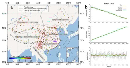
Figure 1.
(a) Distribution and observation duration of continuous observation stations in the six primary tectonic block regions of the Chinese mainland and its vicinity. The observation duration is colour-coded. The station AHAQ is marked by a purple square and labelled by its the name. (b) The observed (gray dots) and modelled (yellow, pink red, blue, and green lines for WN, WN + FN, WN + RW, WN + PN and WN + FN + RW models, respectively) coordinate time series at station AHAQ.
In the GPS data processing, we processed homogeneously using GAMIT software [35], following the processing strategy as that of Zhao et al. [36], We set the elevation cutoff angle to be 10° for all stations, and used the precise ephemeris and clock products from International GNSS Service (IGS), refined absolute antenna phase center models, the GMF tropospheric mapping function, and the ocean tide model FES2004 to reduce various kinds of model errors. We then combined the loosely constrained regional daily solutions with station coordinates with global solutions provided by the Scripps Orbital and Position Analysis Center (SOPAC) using GLOBK software [34] and aligned them into International Terrestrial Reference Frame (ITRF) 2008 using the seven-parameter similarity transformation. Figure 1b shows the coordinate time series at station AHAQ as an instance.
2.2. GPS Coordinate Time Series Fitting
The GPS coordinate time series were analysed using the following model [13]:
where is the station position and represents the linear trend of crustal movement. Coefficients and describe the annual periodic motion, while and describe the semi-annual periodic motion. represents offsets caused by various possible reasons, such as seismic displacement, instrument changes, etc. is the Heaviside step function, and represents the residuals between the observed and modelled time series.
In addition, the Akaike information criterion (AIC) was used to evaluate the effectiveness of noise models by its maximum likelihood value as follows [7]:
where is the number of observations, is the residual time series and is the covariance matrix with its form for the standard power law noise plus white noise as [37],
in which is the amplitude of the driving white noise, is the identity matrix for white noise, and is the covariance matrix for power law noise that depends on the spectral index or − and is scaled by the factor , where is the sampling period in years. The spectral index varies from 0 to 2 for power law noise. Specifically, the white, flicker, and random walk noise have the spectral index of 0, 1, and 2, respectively. It should be noted that different studies use different definitions of the spectral index. For example, Koscielny-Bunde et al. [38] assume that the spectral index equals , where is the Hurst exponent.
The calculation formula of AIC is:
where is the sum of parameters in the design matrix, noise models and the variance of the driving white noise process [37]. Among various noise models or combinations, one with the smallest AIC value is regarded to be the optimal model.
Data gaps or missing data are always caused by instrument failures or gross error elimination, making it impossible to apply the subsequent filtering; therefore, the regularised expectation-maximization (RegEM) was used here to interpolate missing data, due to its peculiar advantage that it does not rely on any additional information, but performs interpolation only according to intrinsic characteristics of data [39].
2.3. Spatiotemporal Filtering Using ICA
ICA, regarded as an extension of PCA, is a blind source signals separation method, which can effectively extract high-order information in coordinate time series. Supposing that m observation signals are linearly combined by n unknown signals, and the ICA model can be expressed by the following equation [22],
where is the number of daily observations, is the matrix composed of residual time series, is the mixing matrix, is the matrix composed of unknown signals, and is the random error or systematic error. Because the statistic characteristics of are unknown, PCA is commonly used as a whitening step to decrease the relevance among its eigenvalues, making eigenvalues with the same variance. For the ICA model, the following assumptions are generally made: First, the unknown original signals are mutually independent. Second, only one of the unknown source signals at most obeys Gaussian distribution. Third, the number of observation signals must be greater than or equal to the number of unknown source signals. In this paper, the FastICA algorithm was adopted to conduct the spatiotemporal filtering, since it has high computational efficiency and good robustness [40].
Besides, the definition of CME is very important in PCA or ICA, and different definitions may lead to different results. In previous PCA or ICA studies, the method proposed by Dong et al. [14] is generally used to define CME in the spatiotemporal filtering; it assumes that if most stations (greater than 50%) have a significant normalised response (greater than 25%) to a PC or IC, then the PC or IC is regarded as one of CME source signals; however, this assumption is not applicable for large regions because it is hard to make most stations influenced by one single source signal as the spatial distance increases. Ming et al. [22] use a spatial analysis method to determine CME, but the method is a little complicated and susceptible to spatial noises, that is, some stations respond weakly to IC signals, but significantly change the spatial distribution pattern. In this paper, ICs are identified as CME source signals if their spatial response has the following characteristics: (1) the IC has the generally uniform spatial distribution characteristics throughout Mainland China. For example, all stations have a comparable response value, or the response value changes smoothly in space; (2) the overall uniform characteristics is not distinctive but regularities are obvious in several local areas, such as the Himalayan region, and the Sichuan-Yunnan region in the Qinghai-Tibetan Plateau block for their strong local effects [20,41]. Once source signals are determined, CME can be calculated by the following formula and then removed in the process of spatiotemporal filtering.
where is the set of ICs, is the element in , and is the spatial response of .
3. Results
3.1. The Optimal Noise Model
According to previous studies on the noise model of GPS time series, the preferred noise model is apt to be characterised by the white noise plus power law noise, which is roughly equivalent to flick noise or the noise with its spectral index close to −1 [6,7,8,9,10,11]; thus, five kinds of noise model combinations were used to analyse GPS coordinate time series from CMONOC by Hector software based on the AIC [37], including white noise only (WN), white noise plus flicker noise (WN + FN), white noise plus random walk noise (WN + RW), white noise plus power law noise (WN + PN), and white noise plus flicker noise plus random walk noise (WN + FN + RW), so as to determine its optimal noise model. The optimal noise model is selected when its AIC value is the smallest, implying the best fitting between the observed and the modelled time series, illustrated in Figure 1b. We calculated all AIC values for each component of the residual time series at each station, and made a detailed statistical analysis, as shown in Figure 2. The result shows that more than 90% of the residual time series are characterised by the optimal noise model combination WN + FN or WN + PN for the east, north and up components. The detailed statistics are as follows: WN + FN and WN + PN account for 83.3% and 7.5% respectively, while WN + FN + RW accounts for 9.2% for east component; WN + FN, WN + PN and WN + FN + RW account for 65.4%, 28.9% and 5.7%, respectively, for north component; WN + PN is the majority, about 74.1%, then WN + FN is 23.7% and the rest is WN + FN + RW, only 2.2% for the up component.
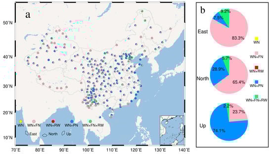
Figure 2.
Distribution (a) and statistics (b) of the optimal noise models of the stations before CME filtering. Different noise models are represented by different colours, including WN (yellow), WN + FN (pink), WN + RW (red), WN + PN (blue) and WN + FN + RW (green). In subplot (a), east, north and up components are indicated by three sectors in the northeast, south and northwest of a circle, respectively. In subplot (b), the percentages mark the proportion of each noise model combination to total noise model combinations.
In addition, we analysed the variations of uncertainties of velocity estimations for each station if the noise model was assumed to be WN only, rather than the optimal noise model determined above. We calculated the uncertainties of velocity estimations for each component at each station based on the WN model and the optimal model, as illustrated in Figure 3. The mean velocity uncertainties are 0.03, 0.02 and 0.06 mm/year for the east, north and up components, respectively, on the WN model, while the corresponding values are 0.41, 0.31 and 0.58 mm/year, respectively, on the optimal noise model. The ratios between the latter and the former are 13.7, 15.5 and 9.7 accordingly, implying that the velocity uncertainties are seriously underestimated on the WN model, or the realistic velocity uncertainties are about an order of magnitude larger than that indicated by the WN model.
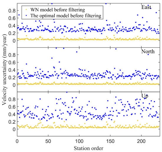
Figure 3.
Velocity uncertainties before CME filtering for each component at each station based on the WN model (yellow dots) and the optimal noise model (blue dots).
3.2. CME Extraction
Before the implementation of CME extraction by ICA, it is necessary to determine the number of principal components (PCs) in the PCA for an improved calculation efficiency. Because the first several PCs represent the majority of signals, the contributions of the following PCs are getting smaller and smaller. The contribution rate of each PC is usually scaled by the ratio of its eigenvalue to the sum of all eigenvalues in the variance matrix [14], we thus calculated eigenvalues and cumulative percentages of the first 30 PCs, as shown in Figure 4. The first several eigenvalues are relatively large for each component, and the eigenvalues of the up component are generally larger than those of the east and north components, implying that CMEs have a larger influence on the up component; meanwhile, the first PC contributes significantly with its percentage of 38.3%, 52.5% and 20.1% for east, north and up components, respectively; the contribution of the following PC decreases gradually as the PC order increases, making the cumulative contribution rate curve tend to be flat. In this paper, PCs with a contribution rate greater than 1.5% were selected as the characteristic components while the increase of cumulative percentage by the following PC was very slow and limited. Finally, the number of PCs was selected to be 8, 8 and 10 for the east, north, and up components, respectively, illustrated in Figure 4. The selected PCs were used for the implementation of the subsequent ICA, so as to decrease the computational burden.
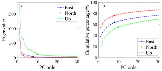
Figure 4.
The first 30 eigenvalues (a) and cumulative variances contribution (b) for east, north and up components, which are represented by blue stars, red triangles and green circles, respectively. The green, blue and red five-pointed stars mark the number of selected PCs for east, north and up components, respectively.
It is also critical to screen out abnormal stations while applying ICA to extract CME, since the existence of these stations will bias the results and greatly affect the stability the results. In previous studies, the inter quartile range (IQR) rule is often used to discern abnormal stations, but this method will not only abandon some abnormal stations, but also a batch of stations with local effects in a certain area [22]. For example, due to strong seasonal movements in the Sichuan-Yunnan region, the overall response of stations in this region is inconsistent with that of stations in other areas of Mainland China; therefore, only some individual abnormal stations that could seriously influence ICA results were abandoned here, in order to avoid the removal of many neighbouring stations that would be influenced by some local effects. Figure 5 shows the normalised independent components (ICs) and their spatial responses for all three components. Obviously, spatial responses by ICs are complex. Some spatial responses are generally uniform throughout Mainland China; some have clear boundaries between the positive and negative spatial responses, and some are slightly chaotic in the entire Mainland China, but show obvious local characteristics, such as in the Sichuan-Yunnan region; these spatial responses are generally in accordance with the characteristics defined before, and thus corresponding ICs can be regarded as CME source signals.
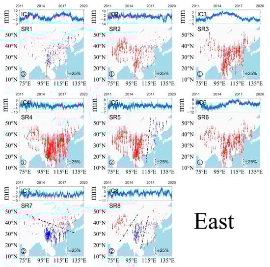
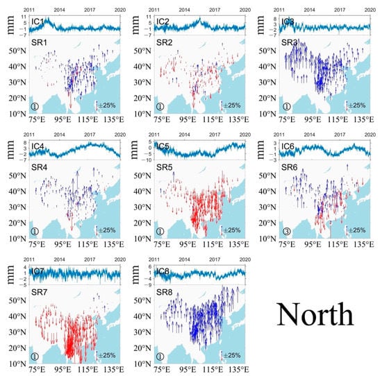
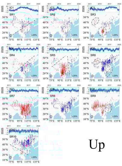
Figure 5.
Normalised ICs and their spatial responses of east, north and up components. Upward and downward arrows represent positive and negative responses, respectively. Spatial responses (SRs) to the corresponding ICs are categorised into three groups, including one with generally uniform characteristics throughout Mainland China (labelled as ① in subplots), one with the smooth variations separated by obvious boundaries between positive and negative responses (labelled as ② in subplots with boundaries indicated by dotted lines), and one with strong local effects (labelled as ③ in subplots with local areas circled by dotted lines).
In addition, the inter-station correlation coefficients and root-mean-square errors (RMSEs) were used to evaluate the effect of ICA in extracting CMEs. Inter-station correlation coefficients can describe the correlation between the residual time series time of stations while RMSEs can describe the SNR of the time series. If CMEs are effectively filtered out, the inter-station correlation coefficients and RMSEs will be significantly reduced. Figure 6 shows the changes in the inter-station correlation coefficients before and after CME filtering. The residual time series before filtering is highly correlated with correlation coefficients varying from 0.23 to 0.56, 0.34 to 0.67 and 0.06 to 0.49 for east, north, and up components respectively and the correlation coefficients gradually decrease to their minimums for all components as the distance between stations increases. After filtering, the correlation coefficients are approximately around 0, indicating that no correlation exists in the filtered residual time series. In addition, mean RMSEs decrease obviously from 3.25, 2.77 and 6.68 mm to 1.92, 1.14 and 3.89 mm with rates of decline of 40.9%, 58.8% and 41.8% before and after filtering for the east, north and up components, respectively, detailed in Table 1; therefore, CME filtering by ICA can effectively remove CMEs and significantly reduce the correlation and noise level of the GPS coordinate time series.
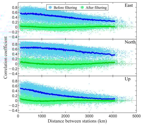
Figure 6.
Inter-station correlation coefficients between the residual time series of stations before and after CME filtering. Correlation coefficients are showed by light blue (before filtering) and light green (after filtering) dots. Their moving averages with a window of 100 km are plotted by dark blue (before filtering) and dark green (after filtering) lines, respectively.

Table 1.
Mean RMSEs of residual time series before and after CME filtering.
4. Discussion
4.1. Characteristics of CME and Its Possible Sources
The distribution characteristics of the spatial response of CME source signals are diverse, as illustrated in Figure 5. Some signals have generally uniform characteristics throughout Mainland China, such as IC2, IC3, IC4, and IC6 of the east component; all ICs except IC3 of the north component; IC7 and IC8 of up component. As for consistent spatial responses in such a large area, these signals should be caused by systematic errors, such as satellite orbit errors, high-order ionospheric delays, frame errors, etc. Some signals cause spatial responses to change smoothly with obvious boundaries between positive and negative responses, such as IC5, IC7 and IC8 of the east component; IC1, IC4, IC5 and IC10 of the up component. These signals may be related to some seasonal and geographic factors, such as monument types and thermal expansions [42]. Some signals have strong responses in local areas, especially in the up component, such as the Tianshan region and Sichuan-Yunnan region (circled by dotted lines) in IC3, the Tianshan region and the southeastern costal region in IC6, and North China block and South China block regions in IC9. These signals may be related to mass loads. For example, Liu et al. [20] regarded atmospheric mass loading and soil moisture mass loading as sources of vertical CME signals in the Sichuan-Yunnan region. Pan et al. [43,44] analysed the vertical crustal deformation in the Tibetan Plateau and Tianshan regions by GPS and GRACE data with consideration of the spatially varying surface seasonal oscillations; it should be noted that the characteristics of spatial responses are sorted and the possible sources are mentioned in this paper, but exact relationships between them are not further explored; this is because the result of the CME filtering is not influenced by the unknown sources of CMEs, and the accurate discrimination of sources of CMEs need more data and the support of other techniques or geophysical mechanisms.
In addition, spectrum analysis of ICs was made to analyse the temporal characteristics of CMEs. Except for some signals with draconitic period and its harmonics [45,46], lower frequency signals were found, including periods of 2048 and 1365.3 days; however, the causes or mechanisms are not clear currently and need to be further analysed on the basis of data with longer duration. Furthermore, the spectral indices of ICs were calculated and listed in Table 2. Nearly all the spectral indices are between 0 and −1 and most of them are close to −1, implying that CME is approximate FN; it is also consistent with the optimal noise model as WN + FN mentioned before.
Table 2.
Spectral indices of ICs.
4.2. The Effect of CME on the Noise Model
It is of great importance to extract CMEs in GPS coordinate time series and remove them to improve the SNR of tectonic signals, especially for some subtle signals. For example, Wdowinski et al. [12] applied spatial filtering to remove CME for analyzing the coseismic and postseismic deformation; thus, it is essential to evaluate the impact of CMEs on noise models. Because the optimal noise model is one of WN + FN, WN + PN and WN + FN + RW before CME filtering, shown in Figure 2b, we reanalysed the optimal noise model from residual time series after applying CME filtering based on the above three noise combination models.
The results show that the majority of the optimal noise model is WN + FN or WN + PN, the same as that before the filtering, but the proportion of FN or PN in the optimal noise model decreases obviously before and after the filtering, illustrated in Figure 7. In WN + FN model, the flicker noise component drops from 6.82, 5.96 and 15.84 to 2.94, 1.93 and 6.07 with a rate of decline of up to 56.9%, 67.6% and 61.7% for east, north and up components, respectively. In WN + PN model, the power law noise component drops from 6.68, 5.66 and 14.19 to 2.89, 1.89 and 6.02 with a rate of decline up to 56.7%, 66.6% and 57.6% for the east, north and up components, respectively. The spectral index of PN is close to −1 with mean values of −0.83, −0.86 and −0.65 for east, north and up components, respectively, implying the WN + PN model is actually close to the WN + FN model. In WN + FN + RW model, the flicker noise component drops from 6.67, 5.93 and 17.78 to 2.78, 1.77 and 6.04 with a rate of decline up to 52.7%, 43.5% and 61.1% for east, north and up components, respectively; thus, FN in the residual time series is the main noise type before the CME filtering and significantly decreased after the CME filtering; it demonstrates, again, that CME is induced by FN.
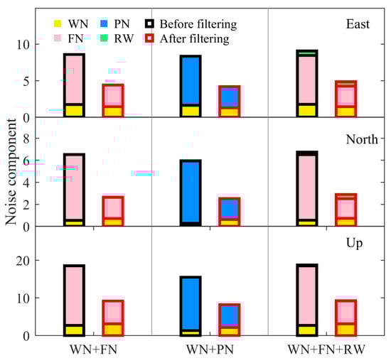
Figure 7.
Noise components in each noise combination model before (black rectangle) and after (red rectangle) CME filtering; it should be noted that units of white noise, flicker noise, power law noise and random walk noise are mm, mm/year 1/4, mm/year −κ/4 and mm/year 1/2, respectively. The y-axis indicates the sum of the magnitude of each noise in the noise combination model.
In addition, as indicated by Figure 7, the portion of WN is small in the noise combination model no matter before or after applying the CME filtering and the magnitude of WN varies slightly after applying the CME filtering; it implies that the CME filtering is able and necessary to reduce the FN.
4.3. The Influence of CME and Noise Model on the Estimation of Crustal Movement Velocity
It is common that estimations in the functional model vary along with variations of the stochastic model and vice versa. As mentioned above, the space-correlated CMEs describe motions of neighbouring stations originating from the same sources, while the time-correlated noises characterise stochastic motions of individual stations. These two factors cause great changes in the stochastic model, leading to changes of estimations in the functional model accordingly. In order to evaluate their influences on estimations of tectonic signals, several versions of estimations are compared based on different stochastic models, including the WN model without applying the CME filtering (WN version), the optimal noise model without (Unfiltered version) and with (Filtered version) applying the CME filtering. Figure 8 shows the velocity field based on the Filtered version (black arrows in Figure 8a,b, detailed in Supplementary Materials), as well as the differentiated velocity field under the Unfiltered and WN versions with relative to the Filtered version, respectively. The average, maximum and minimum differentiated velocity field between the Unfiltered and Filtered versions are 0.15, 1.11 and 0 mm/year for the horizonal (blue arrows in Figure 8c) and 0.13, 1.93 and 0 mm/year for the vertical (blue arrows in Figure 8d), respectively, while those values between the WN and Filtered versions are 0.41, 3.03 and 0.04 mm/year for the horizontal (red arrows in Figure 8c) and 0.36, 2.13 and 0 mm/year for the vertical (red arrows in Figure 8d), respectively; that is also to say, the differences between the WN and Filtered versions are obvious while the differences between the Unfiltered and Filtered versions are small, implying that the velocity estimation would be greatly biased if assuming noise model to be a pure white noise, with comparison to the application of CME filtering or not.
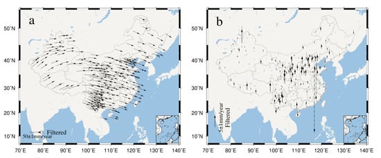
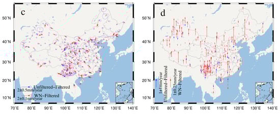
Figure 8.
The horizontal (a) and vertical (b) velocity field based on the optimal noise model with applying the CME filtering (Filtered version) and horizontal (c) and vertical (d) differentiated velocity fields on the optimal noise model without applying the CME filtering (Unfiltered version) and WN model without applying the CME filtering (WN version) with relative to the Filtered version. The black, blue and red arrows show the velocity field of the Filtered version, the differentiated velocity field of the Unfiltered and WN versions relative to the Filtered version, respectively. In subplots b and d, the negative values are shown as the dot-dash-line vectors.
Besides, the precision of three versions of velocity field is discussed by their SNRs. Generally, the WN version has the highest SNRs for each component, and the Filtered version has the higher SNRs than the Unfiltered version, detailed in Table 3. If the average of SNR is taken as an indicator to evaluate the influence of CME and noise model on the velocity estimation, the averaged SNR of the WN version is about 10 dB larger than that of the Unfiltered version, while that of the Filtered version is about 5 dB larger than the Unfiltered version; it is not surprising that the WN version has the largest SNRs since velocity uncertainties have been found underestimated 8–10 times in previous studies [42,43]. As suggested by these studies, it is not proper to estimate the velocity field just based on WN only model and the coloured noise should be considered. Furthermore, the SNRs improve by about 5 dB in the Filtered version, implying that it is necessary to apply CME filtering to estimate crustal movement velocity and other subtle tectonic signals.
Table 3.
SNRs of velocity estimations are based on different versions.
5. Conclusions
Based on coordinate time series with about a decadal duration from 248 continuous stations of CMONOC, we implemented the noise model analysis and CME extraction using ICA, and further discussed the characteristics of CME and its possible sources and influences on the noise model and velocity estimation. The detailed conclusions are summarised as follows:
- The optimal noise models of GPS coordinate time series from CMONOC are mainly characterised by WN + FN and WN + PN. The mean velocity uncertainty estimated in the optimal noise model is about 10 times larger than that in the assumption of WN only, implying the WN model underestimates the velocity uncertainty.
- CME is mainly composed of FN, and its spatial characteristics show that CMEs mainly have uniform influences or smoothly varying influences in Mainland China, while some local CMEs exist in several local regions.
- After applying the CME filtering, the inter-station correlation coefficients decrease significantly, implying ICA filtering can effectively remove CME and greatly reduce the noise level. It is necessary to consider the coloured noise model and CME filtering in the estimation of velocity field by GPS coordinate time series.
However, although the spatiotemporal characteristics of CMEs were analysed based on about a 10-year-long GPS coordinate time series, the sources of CMEs cannot be explained well currently, especially for some lower frequency signals; thus, we will continue our study on the explanation of mechanisms causing CMEs, by using the observations with longer duration and better density.
Supplementary Materials
The following supporting information can be downloaded at: https://www.mdpi.com/article/10.3390/rs14122904/s1, Text S1: Three-Dimensional velocity field in Mainland China based on the consideration of the optimal noise model and the application of CME filtering (Filtered version).
Author Contributions
Conceptualization, K.D.; software, W.Z., P.L. and G.L.; validation, W.Z. and P.L.; writing—original draft preparation, W.Z.; writing—review and editing, K.D., W.Z., P.L., G.L. and Z.M. All authors have read and agreed to the published version of the manuscript.
Funding
This research was funded by National Natural Science Foundation of China (grant numbers 41731071 and 42174012).
Acknowledgments
We are grateful to CMONOC for providing the GPS data, MIT for providing the GAMIT/GLOBK software (version 10.7, http://geoweb.mit.edu/gg/, accessed on 1 September 2020). We also thank editors and four anonymous reviewers for their valuable comments to improve the manuscript. In this paper, some figures with geographical maps were generated with the Generic Mapping Tools (version 5.4.5, http://gmt.soest.hawaii.edu/, accessed on 1 October 2019) and the other figures were generated with MATLAB (version R2019b, https://www.mathworks.com/products/matlab.html, accessed on 1 September 2019).
Conflicts of Interest
The authors declare no conflict of interest.
References
- Zhang, P.; Wang, Q.; Ma, Z. GPS velocity field and active crustal deformation in and around the Tibet Plateau. Earth Sci. Front. 2002, 2, 430–441. [Google Scholar]
- Wang, Q.; You, X.; Wang, W.; Yang, Z. GPS Measurement and Current Crustal Movement Across the Himalaya. Crustal Deform. Earthq. 1998, 18, 43–50. [Google Scholar]
- Zhu, Y.; Chen, Z.; Jiang, G. Preliminary result of crustal movement of China Mainland monitored by using GPS technology. Prog. Astron. 1997, 4, 373–376. [Google Scholar]
- Niu, Z.; Ma, Z.; Chen, X.; Zhang, Z.; Wang, Q.; You, X.; Sun, J. Chinese Crustal Movement Observation Network. J. Geod. Geodyn. 2002, 22, 1–7. [Google Scholar]
- Li, Q.; You, S.; Yang, S.; Du, R.; Qiao, X.; Zou, R.; Wang, Q. A precise velocity field of tectonic deformation in China as inferred from intensive GPS observation. Sci. China Earth Sci. 2012, 55, 695–698. [Google Scholar] [CrossRef]
- Zhang, J.; Bock, Y.; Johnson, H.; Fang, P.; Williams, S.; Genrich, J.; Wdowinski, S.; Behr, J. Southern California permanent GPS geodetic array: Error analysis of daily position estimates and site velocities. J. Geophys. Res. Solid Earth 1997, 102, 18035–18055. [Google Scholar] [CrossRef]
- Williams, S.D.P.; Bock, Y.; Fang, P.; Jamason, P.; Nikolaidis, R.M.; Prawirodirdjo, L.; Miller, M.; Johnson, D.J. Error analysis of continuous GPS position time series. J. Geophys. Res. Solid Earth 2004, 109, B03412. [Google Scholar] [CrossRef] [Green Version]
- Langbein, J. Noise in GPS displacement measurements from Southern California and Southern Nevada. J. Geophys. Res. Solid Earth 2008, 113, B05405. [Google Scholar] [CrossRef]
- Huang, L.; Fu, Y. Analysis on the noises from continuously monitoring GPS sites. Acta Seismol. Sin. 2007, 20, 206–211. [Google Scholar] [CrossRef]
- Tian, Y.; Shen, Z.; Li, P. Analysis on correlated noise in continuous GPS observations. Acta Seismol. Sin. 2010, 32, 696–704. [Google Scholar]
- Wang, W.; Zhao, B.; Qi, W.; Yang, S. Noise analysis of continuous GPS coordinate time series for CMONOC. Adv. Space Res. 2012, 49, 943–956. [Google Scholar] [CrossRef]
- Wdowinski, S.; Bock, Y.; Zhang, J.; Fang, P.; Genrich, J. Southern California permanent GPS geodetic array: Spatial filtering of daily positions for estimating coseismic and postseismic displacements induced by the 1992 Landers earthquake. J. Geophys. Res. Solid Earth 1997, 102, 18057–18070. [Google Scholar] [CrossRef]
- Nikolaidis, R. Observation of Geodetic and Seismic Deformation with the Global Positioning System. Ph.D. Thesis, University of California, San Diego, CA, USA, 2002. [Google Scholar]
- Dong, D.; Fang, P.; Bock, Y.; Webb, F.; Prawirodirdjo, L.; Kedar, S.; Jamason, P. Spatiotemporal filtering using principal component analysis and Karhunen-Loeve expansion approaches for regional GPS network analysis. J. Geophys. Res. Solid Earth 2006, 111, 3405–3421. [Google Scholar] [CrossRef] [Green Version]
- Yuan, L.G.; Ding, X.L.; Chen, W.; Kwok, S.; Chan, S.B.; Hung, P.S.; Chau, K.T. Characteristics of Daily Position Time Series from the Hong Kong GPS Fiducial Network. Chin. J. Geophys. 2013, 51, 976–990. [Google Scholar] [CrossRef]
- Shen, Y.; Li, W.; Xu, G.; Li, B. Spatiotemporal filtering of regional GNSS network’s position time series with missing data using principle component analysis. J. Geod. 2014, 88, 1–12. [Google Scholar] [CrossRef]
- He, X.; Hua, X.; Yu, K.; Wei, X.; Lu, T.; Zhang, W.; Chen, X. Accuracy enhancement of GPS time series using principal component analysis and block spatial filtering. Adv. Space Res. 2015, 55, 1316–1327. [Google Scholar] [CrossRef]
- Li, W.; Shen, Y.; Li, B. Weighted spatiotemporal filtering using principal component analysis for analyzing regional GNSS position time series. Acta Geodaetica et Geophysica 2015, 50, 419–436. [Google Scholar] [CrossRef] [Green Version]
- Yuan, P.; Jiang, W.; Wang, K.; Sneeuw, N. Effects of Spatiotemporal Filtering on the Periodic Signals and Noise in the GPS Position Time Series of the Crustal Movement Observation Network of China. Remote Sens. 2018, 10, 1472. [Google Scholar] [CrossRef] [Green Version]
- Liu, B.; Dai, W.; Peng, W.; Meng, X. Spatiotemporal analysis of GPS time series in vertical direction using independent component analysis. Earth Planets Space 2015, 67, 189. [Google Scholar] [CrossRef] [Green Version]
- Ming, F.; Yang, Y.; Zeng, A. Analysis and comparison of common mode error extraction using principal component analysis and independent component analysis. J. Geod. Geodyn. 2017, 37, 385–389. [Google Scholar]
- Ming, F.; Yang, Y.; Zeng, A.; Zhao, B. Spatiotemporal filtering for regional GPS network in China using independent component analysis. J. Geod. 2017, 91, 419–440. [Google Scholar] [CrossRef]
- Wu, W.; Meng, G.; Wu, J.; Zhao, G. Optimizing realization of the terrestrial reference frame on a regional basis: A case study using the crustal movement observation network of China. Adv. Space Res. 2021, 68, 2367–2382. [Google Scholar] [CrossRef]
- Wu, J.; Wang, Y.; Wu, W. Analysis of current crustal movement velocity field of south-eastern Tibetan Plateau. J. Geod. Geodyn. 2018, 38, 116–124. [Google Scholar]
- Liang, S.; Gan, W.; Shen, C.; Xiao, G.; Liu, J.; Chen, W.; Ding, X.; Zhou, D. Three-dimensional velocity field of present-day crustal motion of the Tibetan Plateau derived from GPS measurements. J. Geophys. Res. Solid Earth 2013, 118, 5722–5732. [Google Scholar] [CrossRef]
- Dang, Y.; Yang, Q.; Xue, S.; Yue, C.; Liu, Z. GNSS monitoring dynamic variation characteristics of crustal deformation in the Sichuan-Yunnan REGION. J. Geod. Geodyn. 2019, 39, 111–116. [Google Scholar]
- Wei, Z.; Zhao, L. Lg-Q model and its implication on high-frequency ground motion for earthquakes in the Sichuan and Yunnan region. Earth Planet. Phys. 2019, 3, 526–536. [Google Scholar] [CrossRef]
- Liu, R.; Zou, R.; Li, J.; Zhang, C.; Zhao, B.; Zhang, Y. Vertical displacements driven by groundwater storage changes in the north China plain detected by GPS observations. Remote Sens. 2018, 10, 259. [Google Scholar] [CrossRef] [Green Version]
- Yu, J.; Tan, K.; Zhang, C.; Zhao, B.; Wang, D.; Li, Q. Present-day crustal movement of the Chinese mainland based on Global Navigation Satellite System data from 1998 to 2018. Adv. Space Res. 2019, 63, 840–856. [Google Scholar] [CrossRef]
- Peng, Z.; Wang, B.; Shao, Y.; Li, E. Calculation of Crustal Horizontal Strain in Central North China Based on Refined Multiquadric Function and the Spherical Integral Strain Method. Earthq. Res. China 2019, 35, 76–83. [Google Scholar]
- Ma, J.; Li, Z.; Jiang, W.; Cao, C.; Huo, L.; Zhou, X. A new three-dimensional noise modeling method based on singular value decomposition and its application to CMONOC GPS network. Earth Space Sci. 2021, 8, e2020EA001250. [Google Scholar] [CrossRef]
- Li, C.; Huang, S.; Chen, Q.; Dam, T.; Fok, H.; Zhao, Q.; Wu, W.; Wang, X. Quantitative evaluation of environmental loading induced displacement products for correcting GNSS time series in CMONOC. Remote Sens. 2020, 12, 594. [Google Scholar] [CrossRef] [Green Version]
- Yao, C.; Liu, L.; Lin, X.; Wang, C.; Zhang, R.; Wang, J.; Chen, R. Analyzing typhoon-triggered vertical land motion from GPS and environmental load-induced deformation data. Chin. J. Geophys.-Chin. Ed. 2020, 63, 2870–2881. [Google Scholar]
- Zhang, P.; Deng, Q.; Zhang, G.; Ma, J.; Gan, W.; Min, W.; Mao, F.; Wang, Q. Active tectonic blocks and strong earthquakes in the continent of China. Sci. China Ser. D Earth Sci. 2003, 46, 13–24. [Google Scholar]
- Herring, T.A.; King, R.W.; McClusky, S.C. Documentation of the GAMIT and GLOBK Software Release 10.4; Massachusetts Institute of Technology: Cambridge, MA, USA, 2010. [Google Scholar]
- Zhao, B.; Huang, Y.; Zhang, C.; Wang, W.; Tan, K.; Du, R. Crustal deformation on the Chinese mainland during 1998–2014 based on GPS data. Geod. Geodyn. 2015, 6, 7–15. [Google Scholar] [CrossRef] [Green Version]
- Bos, M.S.; Fernandes, R.M.S.; Williams, S.D.P.; Bastos, L. Fast Error Analysis of Continuous GNSS Observations with Missing Data. J. Geod. 2013, 87, 351–360. [Google Scholar] [CrossRef] [Green Version]
- Koscielny-Bunde, E.; Bunde, A.; Havlin, S.; Roman, H.E.; Goldreich, Y.; Schellnhuber, H.-J. Indication of a universal persistence law governing atmospheric variability. Phys. Rev. Lett. 1998, 81, 729–732. [Google Scholar] [CrossRef]
- Schneider, T. Analysis of Incomplete Climate Data: Estimation of Mean Values and Covariance Matrices and Imputation of Missing Values. J. Clim. 2001, 14, 853–871. [Google Scholar] [CrossRef]
- Hyvarinen, A. Fast and robust fixed-point algorithms for independent component analysis. IEEE Trans. Neural Netw. 1999, 10, 626–634. [Google Scholar] [CrossRef] [Green Version]
- Khandelwal, D.D.; Gahalaut, V.; Kumar, N.; Kundu, B.; Yadav, R.K. Seasonal variation in the deformation rate in NW Himalayan region. Nat. Hazards 2014, 74, 1853–1861. [Google Scholar] [CrossRef]
- Wang, W.; Qiao, X.; Wang, D.; Chen, Z.; Yu, P.; Lin, M.; Chen, W. Spatiotemporal noise in GPS position time-series from Crustal Movement Observation Network of China. Geophys. J. Int. 2019, 216, 1560–1577. [Google Scholar] [CrossRef]
- Pan, Y.; Shen, W.; Shum, C.K.; Chen, R. Spatially varying surface seasonal oscillations and 3-D crustal deformation of the Tibetan Plateau derived from GPS and GRACE data. Earth Planet. Sci. Lett. 2018, 502, 12–22. [Google Scholar] [CrossRef]
- Pan, Y.; Chen, R.; Yi, S.; Wang, W.; Ding, H.; Shen, W.; Chen, L. Contemporary mountain-building of the Tianshan and its relevance to geodynamics constrained by integrating GPS and GRACE measurements. J. Geophys. Res. Solid Earth 2019, 124, 12171–12188. [Google Scholar] [CrossRef]
- Amiri-Simkooei, A.R. On the nature of GPS draconitic year periodic pattern in multivariate position time series. J. Geophys. Res. Solid Earth 2013, 118, 2500–2511. [Google Scholar] [CrossRef] [Green Version]
- Ray, J.; Altamimi, Z.; Collilieux, X.; Dam, T.V. Anomalous harmonics in the spectra of GPS position estimates. GPS Solut. 2008, 12, 55–64. [Google Scholar] [CrossRef]
Publisher’s Note: MDPI stays neutral with regard to jurisdictional claims in published maps and institutional affiliations. |
© 2022 by the authors. Licensee MDPI, Basel, Switzerland. This article is an open access article distributed under the terms and conditions of the Creative Commons Attribution (CC BY) license (https://creativecommons.org/licenses/by/4.0/).