Communication

PARAFAC Estimators for Coherent Targets in EMVS-MIMO Radar with Arbitrary Geometry

1
Hubei Key Laboratory of Intelligent Vision Based Monitoring for Hydroelectric Engineering, China Three Gorges University, Yichang 443002, China
2
College of Computer and Information Technology, China Three Gorges University, Yichang 443002, China
3
College of Physical Science and Engineering, Yichun University, Yichun 336000, China
4
College of Electronic Countermeasure, National University of Defense Technology, Hefei 230037, China
*
Author to whom correspondence should be addressed.
Remote Sens. 2022, 14(12), 2905; https://doi.org/10.3390/rs14122905
Submission received: 29 April 2022 / Revised: 14 June 2022 / Accepted: 15 June 2022 / Published: 17 June 2022
(This article belongs to the Special Issue Small or Moving Target Detection with Advanced Radar System)

Abstract

:
In the past few years, multiple-input multiple-output (MIMO) radar with electromagnetic vector sensor (EMVS) array, or called EMVS-MIMO radar, has attracted extensive attention in target detection. Unlike the traditional scalar sensor-based MIMO radar, an EMVS-MIMO radar can not only provides a two-dimensional (2D) direction finding of the targets but also offers 2D polarization parameter estimation, which may be important for detecting weak targets. In this paper, we investigate into multiple parameter estimations for a bistatic EMVS-MIMO radar in the presence of coherent targets, whose transmitting EMVS and receiving EMVS are placed in an arbitrary topology. Three tensor-aware spatial smoothing estimators are introduced. The core of the proposed estimators is to de-correlate the coherent targets via the spatial smoothing technique and then formulate the covariance matrix into a third-order parallel factor (PARAFAC) tensor. After the PARAFAC decomposition of the tensor, the factor matrices can be obtained. Thereafter, the 2D direction finding can be accomplished via the normalized vector cross-product technique. Finally, the 2D polarization parameter can be estimated via the least squares method. Unlike the state-of-the-art PARAFAC estimator, the proposed estimators are suitable for arbitrary sensor geometries, and they are robust to coherent targets as well as sensor position errors. In addition, they have better estimation performance than the current matrix-based estimators. Moreover, they are computationally efficient than the current subspace methods, especially in the presence of a large-scale sensor array. In addition, the proposed estimators are analyzed in detail. Numerical experiments coincide with our theoretical findings.

Graphical Abstract

1. Introduction

Multiple-input multiple-output (MIMO) radar has attracted widespread attention in remote sensing. MIMO radar is characterized by multiple transmitting (Tx) sensors and multiple receiving (Rx) sensors [1]. A MIMO radar emits mutual orthogonal waveforms and receives the echoes simultaneously [2]. The waveform diversity enables a MIMO radar to achieve better performance than a phased-array radar in noise suppression, interference elimination, and parameter identifiability [3]. Among various kinds of MIMO radars, the bistatic MIMO radar is attractive as the Tx array and the Rx array are separated [4]. Benefitting from such a configuration, a bistatic MIMO radar would have better survival ability than a monostatic one in military applications.
The issue of direction-of-departure (DOD) and direction-of-arrival (DOA) estimation is critical to a bistatic MIMO radar. Many efforts have been devoted to this topic in the past decades. A lot of super-resolution algorithms have been reported, for instance, estimation approach to signal parameters with rotational invariance technique (ESPRIT) [5,6], spatial spectrum peak search [7,8,9], and tensor methods [10,11,12,13]. Generally speaking, tensor-aware methods provide much better performance than the matrix-based one [14,15,16,17,18,19], since the multidimensional structure of the array measurement can be taken into consideration by the latter. However, most of the current algorithms mainly focus on the one-dimensional (1D) direction estimation issue by using the 1D scalar linear array, e.g., uniform linear array (ULA), and non-uniform linear array (nested array, coprime array). In engineering applications, two-dimensional (2D) direction estimation, i.e., 2D-DOD and 2D-DOA estimation, is more attractive than the former. It is well-known that in order to obtain 2D angle estimation using the scalar-array-based MIMO radar, non-linear Tx arrays and Rx arrays must be adopted [20,21,22,23], e.g., rectangular array, circular array, arbitrary array. Unfortunately, these nonlinear scalar geometries are usually too complex to be conformal with the platform. In addition, the calibration of the model errors will become more complicated due to the irregular geometries [24,25].
On the other hand, the electromagnetic vector sensor (EMVS) array has brought new insight into direction estimation [26,27,28,29]. A complete EMVS occupies six components: three of them measure the electric-field and three of them sense the magnetic-field. Unlike the traditional scalar array, an EMVS array not only provides 2D direction estimation, but it also offers the polarization status of the incoming source. The EMVS array enables the MIMO radar to obtain 2D direction estimation as well as 2D polarization estimation of the targets. A bistatic EMVS-MIMO radar was introduced in [30], whose Tx array and Rx array are both ULA. Therein, an ESPRIT algorithm was introduced to estimate the 2D-DOD, the 2D-DOA, the 2D Tx polarization angle (2D-TPA) and the 2D Rx polarization angle (2D-RPA). Another ESPRIT algorithm was proposed in [31], which can avoid the aperture loss in [30]. A parallel factor (PARAFAC) estimator was designed in [32], in which the tensor nature of the array measurement was taken into account, and it offers much better estimation performance than those matrix approaches. In [33], the coprime array geometry-based Tx/Rx configuration was considered for EMVS-MIMO radar. Benefitting from the larger sensor aperture, it offers more accurate estimation performance than the ULA setup. In [34], an arbitrary Tx/Rx geometry was investigated for EMVS-MIMO radar. An ESPRIT-like estimator based on the normalized vector cross-product technique has been given, which is capable of providing closed-form solutions for 2D-DOD, 2D-DOA, 2D-TPA and 2D-RPA estimation. In addition, it is insensitive to the sensor position errors.
The above-mentioned algorithms are only suitable for uncorrelated targets scenario, which is often inappropriate in practice. In the presence of coherent targets, there will be a rank deficient in the array measurement. To alleviate this issue, the polarization smoothing was performed in [35], which resolves the coherent targets via smoothing the array measurement along the polarization domain. A polarization difference smoothing framework was presented in [36], which is suitable for nonstationary noise. Nevertheless, both [35,36] would sacrifice the polarization information of the targets. To avoid such drawback, the generalized spatial smoothing framework was carried out in [37]. Three spatial smoothing approaches, named Tx smoothing (TS), Rx smoothing (RS), and Tx/Rx smoothing (TRS), were derived, which are suitable for arbitrary Tx/Rx geometry. However, the eigendecomposition of TS, RS and TRS are computationally inefficient. In addition, since the tensor nature has been ignored, the estimation accuracy of these approaches can be improved further.
In this paper, tensor-aware approaches are proposed to tackle the coherent targets problem in bistatic EMVS-MIMO radar. More specifically, the contributions of this paper are listed as follows:
(1)
The generalized spatial smoothing-based tensor models are established. The core of the proposed algorithm is to solve the rank-deficiency issue via spatial smoothing. To utilize the multi-dimensional structure of the array measurement, the array data after smoothing is rearranged into a third-order PARAFAC tensor. Unlike the state-of-the-art PARAFAC estimator in [32], the improved PARAFAC approaches are robust to coherent targets owing to the spatial smoothing. In addition, since the third-order PARAFAC decomposition can be quickly accomplished via the existing COMFAC algorithm, the proposed frameworks are more effective than the existing fourth-order PARAFAC algorithms [12].
(2)
The ESPRIT-like strategies are developed for joint 2D-DOD, 2D-DOA, 2D-TPA and 2D-RPA estimation. After PARAFAC decomposition, the factor matrices that form the tensor are achieved. The 2D-DOD and 2D-DOA are estimated via the normalized vector cross-product technique. Thereafter, 2D-TPA and 2D-RPA are achieved via the least squares (LS) with the previously estimated 2D-DOD and 2D-DOA. All the estimated parameters are in closed-form and paired automatically. Since the multi-dimensional structure has been explored, they outperform the matrix-based smoothing methods in [37]. Furthermore, as the 2D-DOD and 2D-DOA estimation rely on the normalized vector cross-product technique instead of the uniformity of the sensor array, the proposed approaches are suitable for arbitrary geometries and sensor position errors, while the PARAFAC estimator in [32] is only effective for the ULA configuration.
(3)
The advantages of the proposed approaches are verified via theoretically analysis and simulations. The proposed approaches are analyzed with respect to computational complexity, identifiability, as well as the Cramer–Rao Bound (CRB). Computer simulations are designed to show its effectiveness.

2. Tensor and Problem Formulation

2.1. Tensor and PARAFAC Decomposition

The following preliminaries concerning tensor and tensor decomposition will be utilized throughout this paper. Readers that are interested in more details on the tensor are referred to [38].
Definition 1.
An I 1 × I 2 × × I N tensor has N degrees-of-freedom or indices. The mode-n unfolding of X I 1 × I 2 × × I N is given by [ X ] ( n ) , which unfolds a tensor into a matrix, where the ( i 1 , i 2 , , i N ) -entity of X is the ( i n , p ) -th entity of [ X ] ( n ) , where p = 1 + k = 1 , k n N ( i k 1 ) J k with  J k = m = 1 , m n k 1 I m .
Definition 2.
The mode-n product of matrix A J n × I n and X I 1 × I 2 × × I N is given by Y = X × n A , which satisfies:
[ Y ] ( n ) = A [ X ] ( n )
Definition 3.
The PARAFAC decomposition of a rank-K tensor X I 1 × I 2 × × I N is given by
X = k = 1 K a k ( 1 ) a k ( 2 ) a k ( N ) = I × 1 A × 2 ( 1 ) A × 3 ( 2 ) A × N ( N 1 ) A ( N )
where denotes the outer-product, I I 1 × I 2 × × I N is the identical tensor, a k ( n ) I n × 1 ( n = 1 , 2 , , N ) is a rank-one vector, and A ( n ) = [ a 1 ( n ) , a 1 ( n ) , , a K ( n ) ] is the so-called factor matrix. In matrix format, (2) is also given by
[ X ] ( n ) = A n [ A n + 1 A N A 1 A n 1 ] T
where denotes the Khatri–Rao product, and ( ) T denotes transpose.
Definition 4.
For the PARAFAC decomposition in (2), define the order set O j = { o j , 1 , o j , 2 , , o j , M j } , j = 1 , 2 , , J , which denotes a partitioning of the dimensions O = { 1 , 2 , , N } , a new PARAFAC tensor X O 1 , O 2 , , O J T 1 × T 2 × × T J can be obtained via combining the rank-one vectors according to the order set as [39]:
X O 1 , O 2 , , O J = k = 1 K b k ( 1 ) b k ( 2 ) b k ( J )
where T j = Π m = 1 M j I o j , m , b k ( j ) = a k ( o j , M j ) a k ( o j , M j 1 ) a k ( o j , 1 ) , and denotes the Kronecker product.

2.2. Signal Model

Consider a bistatic EMVS-MIMO radar with arbitrary sensor geometry, as shown in Figure 1. Without loss of generality, we assume that there are M-element colocated transmitting EMVSs and N-element colocated receiving EMVSs. The positions with respect to the m-th ( m = 1 , 2 , , M ) Tx EMVS and the n-th ( n = 1 , 2 , , N ) EMVS are denoted by p t , m [ x t , m , y t , m , z t , m ] T and p r , n [ x r , n , y r , n , z r , n ] T , respectively. Supposing that K far-field targets appearing in same range bin, the 2D-DOD, 2D-DOA, 2D-TPA, and 2D-RPA of the k-th ( k = 1 , 2 , , K ) target are denoted by ( θ r , k , ϕ r , k ) , ( θ t , k , ϕ t , k ) , ( γ r , k , η r , k ) and ( γ t , k , η t , k ) , where θ t , k and θ r , k are the Tx elevation angle and the Rx elevation angle, respectively, ϕ t , k and ϕ r , k are the Tx azimuth angle and the Rx azimuth angle, respectively, γ t , k and γ r , k are the Tx auxiliary polarization angle and the Rx auxiliary polarization angle, respectively, and η t , k and η r , k are the Tx polarization phase difference and the Rx polarization phase difference, respectively.
Suppose that the Tx array emit 6 M mutual orthogonal pulse waveforms w ( t , τ ) = [ w 1 ( t , τ ) , w 2 ( t , τ ) , , w 6 M ( t , τ ) ] T , i.e.,
T w m ( t , τ ) w n * ( t , τ ) d τ = δ ( m n )
where t denotes the pulse index, τ denotes the fast time index, ( ) * denotes conjugate, T denotes the pulse duration, and δ ( ) denotes the Kronecker delta. In the presence of orthogonal waveforms assumption, the array outputs from the matched filters are given by [31,32]:
x ( t ) = k = 1 K [ a t , k b t , k a r , k b r , k ] s k ( t ) + n ( t ) = [ A t B t A r B r ] s ( t ) + n ( t )
where A t = [ a t , 1 , a t , 2 , , a t , K ] , A r = [ a r , 1 , a r , 2 , , a r , K ] ; B t = [ b t , 1 , b t , 2 , , b t , K ] and B r = [ b r , 1 , b r , 2 , , b r , K ] ; s ( t ) = [ s 1 ( t ) , s 2 ( t ) , , s K ( t ) ] T denotes the target reflection coefficient vector; n ( t ) denotes the additive white Gaussian noise (AWGN) vector with variance is σ 2 , namely, E { n ( t ) n H ( t ) } = σ 2 I 36 M N , where ( ) H denotes conjugate transpose, I 36 M N denotes the 36 M N × 36 M N identity matrix, and E { } is the mathematical expectation; a t , k = [ 1 , e j 2 π τ t 2 , k / λ , , e j 2 π τ t M , k / λ ] T M × 1 denotes the k-th Tx spatial steering vector, τ t m , k = p t , m T r t , k with r t , k = [ sin θ t , k cos ϕ t , k , sin θ t , k sin ϕ t , k , cos θ t , k ] T ; a r , k = [ 1 , e j 2 π τ r 2 , k / λ , , e j 2 π τ r N , k / λ ] T N × 1 denotes the k-th Rx spatial steering vector, τ r n , k = p r , n T r r , k with r r , k = [ sin θ r , k cos ϕ r , k , sin θ r , k sin ϕ r , k , cos θ r , k ] T ; and b t / r , k 6 × K denote the k-th Tx/Rx polarization response vector, which is given by
b t / r , k = [ cos ϕ t / r , k cos θ t / r , k sin γ t / r , k e j η t / r , k sin ϕ t / r , k cos γ t / r , k sin ϕ t / r , k cos θ t / r , k sin γ t / r , k e j η t / r , k + cos ϕ t / r , k cos γ t / r , k sin θ t / r , k sin γ t / r , k e j η t / r , k sin ϕ t / r , k sin γ t / r , k e j η t / r , k cos ϕ t / r , k cos θ t / r , k cos γ t / r , k cos ϕ t / r , k sin γ t / r , k e j η t / r , k sin ϕ t / r , k cos θ t / r , k cos γ t / r , k sin θ t / r , k cos γ t / r , k ] } e t / r , k 3 × 1 } m t / r , k 3 × 1
where e t / r , k denotes the electric-field response vector, and m t / r , k denotes the magnetic-field components. Moreover, the vector cross-products with respect to e t , k , m t , k and e r , k , m r , k are given by the normalized Poynting-vector as:
e t , k e t , k F m t , k * m t , k F = r t , k , e r , k e r , k F m r , k * m r , k F = r r , k
where denotes the vector cross-product, and F denotes the Frobenius norm. In addition, the b t , k and b r , k can be factorized as:
b t , k = F t , k v t , k , b r , k = F r , k v r , k
where F t , k and F r , k are direction-dependent-only matrices, and v t , k and v r , k are polarization dependent-only vectors, which are given below:
F t , k = [ cos ϕ t , k cos θ t , k sin ϕ t , k sin ϕ t , k cos θ t , k cos ϕ t , k sin θ t , k 0 sin ϕ t , k cos ϕ t , k cos θ t , k cos ϕ t , k sin ϕ t , k cos θ t , k 0 sin θ t , k ] , v t , k = [ sin γ t , k e j η t , k   cos γ t , k ]
Define C t = A t B t , C r = A r B r . In addition, suppose that the noise vector n ( t ) is uncorrelated with the target reflection coefficient vector s ( t ) ; then, the covariance matrix of x ( t ) is given by:
R = E { x ( t ) x H ( t ) } = [ C t C r ] R s [ C t C r ] H + σ 2 I 36 M N
where R s = E { s ( t ) s H ( t ) } is the mathematical expectation of s ( t ) . In the presence of correlated targets, R s is rank deficient, i.e., r a n k { R s } < K , r a n k { } returns the rank of a matrix. Consequently, the noise R is also rank deficient and yields ill signal subspace. As a result, the subspace methods in [30,31,33,34] will fail to work, and the PARAFAC method in [33] cannot correctly operate either.

3. The Proposed PARAFAC Estimators

3.1. Review of the Generalized Spatial Smoothing Approaches

The core idea of the generalized spatial smoothing approaches is to smooth the array measurement along the spatial domain [37]. According to the mechanism of spatial smoothing, the generalized spatial smoothing approaches can be divided into three categories, namely, the transmitting smoothing-based (TS) approach, the receiving smoothing-based (RS) approach, and the transmitting–receiving-smoothing-based (TRS) approach. The TS approach relies on smoothing the array measurement along the Tx direction. Let x t , m ( t ) denotes the array measurement corresponding to the m-th Tx EMVS, i.e.,
x t , m ( t ) = [ B t C r ] S m { A t } s ( t ) + n t , m ( t )
where n t , m ( t ) is the corresponding noise vector, and S m { A t } returns a diagonal matrix whose diagonal elements are the m-th row of A t . Accordingly, the covariance matrix of x t , m ( t ) is given by
R t , m = E { x t , m ( t ) x t , m H ( t ) } = [ B t C r ] S m { A t } R s S m H { A t } [ B t C r ] H + σ 2 I 36 N
Thereafter, a TS matrix R t can be constructed via averaging all the R t , m , i.e.,
R t = 1 / M m = 1 M R t , m = [ B t C r ] R s , t [ B t C r ] H + σ 2 I 36 N
where R s , t = 1 / M m = 1 M S m { A t } R s S m H { A t } . According to [40], R s , t is full rank if M K and ( θ t , k , ϕ t , k ) are distinct. Accordingly, the rank of the noiseless R t is K, and then the subspace-based ESPRIT is capable for parameter estimation.
Likewise, we can pick up the array measurement associated with the n-th Rx EMVS, which is given by
x r , n ( t ) = [ C t B r ] S n { A r } s ( t ) + n r , n ( t )
where n r , n ( t ) accounts for the associated noise vector. Thereafter, we can construct an RS matrix R r via averaging all the covariance matrices of x r , n ( t ) (denoted by R r , n ), i.e.,
R r = 1 / N n = 1 N R r , n = [ C t B r ] R s , r [ C t B r ] H + σ 2 I 36 M
where R s , r = 1 / N n = 1 N S n { A r } R s S n H { A r } . Obviously, the rank of the noiseless R r is K if N K and ( θ r , k , ϕ r , k ) are distinct.
In addition, we can choose the array measurement associate with the m-th Tx EMVS and the n-th Rx EMVS, which is given by
x t r , m , n ( t ) = [ B t B r ] S m { A t } S n { A r } s ( t ) + n t r , m , n ( t )
where n t r , m , n ( t ) represents the corresponding noise vector. Let the covariance matrix of x t r , m , n ( t ) is R t r , m , n . Similarly, the TRS approach is based on the averaging all the R t r , m , n , i.e.,
R t r = 1 / M N n = 1 N m = 1 M R t r , m , n = [ B t B r ] R s , t r [ B t B r ] H + σ 2 I 36
where R s , t r = 1 / N M n = 1 N m = 1 M S n { A r } S m { A t } R s S n H { A r } S m H { A t } . In addition, the rank of the noiseless R t r should be K once M N K and ( θ t , k , ϕ t , k ) , ( θ r , k , ϕ r , k ) are distinct. In practice, R t , R r , and R t r can be estimated via L snapshots as:
R ^ t = 1 / M L l = 1 L m = 1 M x t , m ( l ) x t , m H ( l ) R ^ r = 1 / N L l = 1 L n = 1 N x r , n ( l ) x r , n H ( l ) R ^ t r = l = 1 L m = 1 M n = 1 N x t r , m , n ( l ) x t r , m , n H ( l )
Essentially, the TS approach is only smoothing the data measurements along the Tx spatial direction. The RS approach, on the other hand, is only smoothing them along the Rx spatial direction. Finally, the TRS approach is smoothing the data in both Tx and Rx directions.
The existing subspace-based approaches rely on the eigen decomposition of the estimated covariance matrices, which are computationally inefficient. Since the tensor nature is ignored, the estimation accuracy can be improved further. In what follows, we will introduce the PARAFAC-based estimators, which can avoid the above drawbacks.

3.2. PARAFAC Models and PARAFAC Decomposition

For the covariance data model in (14), it can be formulated as a fourth-order PARAFAC model as:
R = I × 1 B t × 2 C r × 3 B t × 4 * ( C r * R s , t ) + N
where N is the tensor version of σ 2 I 36 N . Actually, R s , t can be combined with any of the four factor matrices B t , C r , B t * and C r * . The estimation of the factor matrices can be accomplished via optimizing the following:
B t , C r = arg min ^ I × 1 B t × 2 C r × 3 B t × 4 * ( C r * R s , t ) F 2
where R ^ denotes the arranged R ^ t . Although the above issue can be solved via the quadrilinear alternative least squares (ALS) algorithm, it suffers from the slowness of the convergence speed. Inspired by the fact that there exists a fast algorithm, named COMFAC, for a third-order PARAFAC model, R can be arranged into a third-order PARAFAC model. For the PARAFAC model in (20), define O 1 = { 1 } , O 2 = { 2 } , and O 3 = { 3 , 4 } . According to Definition 4, we can obtain another PARAFAC model as:
R t = I × 1 B t × 2 C r × 3 D t + N t
where D t = B t * C r * R s , t , N t denotes the arranged array noise. Similarly, we can obtain the rearranged array tensor R r and R t r as:
R r = I × 1 C t × 2 B r × 3 D r + N r
R t r = I × 1 B t × 2 B r × 3 D t r + N t r
where D r = C t * B r * R s , r , D t r = B t * B r * R s , t r , N r and N t r denotes the rearranged array noise.
Taking the model in (22) as an example, we will show how to obtain the factor matrices from the third-order PARAFAC tensor. Obviously, the factor matrices of R t can be achieved via solving:
B t , C r , D t = arg min R ^ t I × 1 B t × 2 C r × 3 D t F 2
On the other hand, the PARAFAC tensor R t in (22) can be unfolded into matrix format as
X 1 = [ R t ] ( 1 ) T = [ C r D t ] B t T + N 1 X 2 = [ R t T ] ( 2 ) T = [ D t B t ] C r T + N 2 X 3 = [ R t ] ( 3 ) T = [ B t C r ] D t T + N 3
where N 1 = [ N t ] ( 1 ) T , N 2 = [ N t ] ( 2 ) T and N 3 = [ N t ] ( 3 ) T . As a result, the optimization in (25) can be rewritten as joint optimize:
B t , C r , D t = { arg min X ^ 1 [ C r D t ] B t T F 2 arg min X ^ 2 [ D t B t ] C r T F 2 arg min X ^ 3 [ B t C r ] D t T F 2
The trilinear alternating least squares (TALS) is a popular solver of the joint optimization issue in (27). TLAS treats each sub-issue as a least squares (LS) problem and assumes two of the factor matrices are known. Then, it obtains the third factor matrix via LS successively. The LS fitting will repeat until algorithm convergence. Mathematically, the LS updates of B t , C r , and D t are given by:
{ B ^ t T = [ C r D t ] X ^ 1 C ^ r T = [ D r B t ] X ^ 2 D ^ t T = [ B r C t ] X ^ 3
Usually, the convergence condition is set to X ^ 1 [ C r D t ] B t T F 2 ξ or the iteration steps are larger than a given integer; ξ denotes a given threshold. Moreover, the COMFAC algorithm is often adopted [41], which only require a few iteration steps. Denote the Kruskal ranks of B t , C r , and D t as K R { B t } , K R { C r } , and K R { D t } , respectively. It has been pointed out in [38] that if
K R { B t } + K R { C r } + K R { D t } 2 K + 2
then the estimates of B t , C r , and D t are unique to permutations and scaling effects of columns, i.e.,
{ B ^ t = B t Π 1 Δ 1 + E 1 C ^ r = C r Π 1 Δ 2 + E 2 D ^ t = D t Π 1 Δ 3 + E 3
where Π 1 denotes a permutation matrix, and Δ 1 , Δ 2 , and Δ 3 denote the diagonal matrices with Δ 1 Δ 2 Δ 3 = I K . E 1 , E 2 , and E 3 account for the associated fitting errors.
For the RS approach, the matrix unfolding of R r is given by
Y 1 = [ R r ] ( 1 ) T = [ B r D r ] C t T + N 1 Y 2 = [ R r ] ( 2 ) T = [ D r C t ] B r T + N 2 Y 3 = [ R r ] ( 3 ) T = [ C t B r ] D r T + N 3
where N 1 = [ N r ] ( 1 ) T , N 2 = [ N r ] ( 2 ) T , and N 3 = [ N r ] ( 3 ) T are the noise matrices. Accordingly, the factor matrices that formed R r can be formulated as joint optimizers:
B r , D r , C t = { arg min Y ^ 1 [ B r D r ] C t T F 2 arg min Y ^ 2 [ D r C t ] B r T F 2 arg min Y ^ 3 [ C t B r ] D r T F 2
Similarly, the LS updates of C t , B r , and D r are given by:
{ C ^ t T = [ B r D r ] Y ^ 1 B ^ r T = [ D r C t ] Y ^ 2 D ^ r T = [ C t B r ] Y ^ 3
The estimated factor matrices of R r can be formulated as:
{ C ^ t = C t Π 2 Δ 1 + E 1 B ^ r = B r Π 2 Δ 2 + E 2 D ^ r = D r Π 2 Δ 3 + E 3
where Δ 1 , Δ 2 , and Δ 3 are diagonal matrices, and E 1 , E 2 , and E 3 are fitting errors.
For the TRS approach, the matrix unfolding of R t r can be written as:
Z 1 = [ R t r ] ( 1 ) T = [ B r D t r ] B t T + N 1 Z 2 = [ R t r ] ( 2 ) T = [ D t r B t ] B r T + N 2 Z 3 = [ R t r ] ( 3 ) T = [ B t D r ] D t r T + N 3
where N 1 = [ N t r ] ( 1 ) T , N 2 = [ N t r ] ( 2 ) T and N 3 = [ N t r ] ( 3 ) T . Similarly, the factor matrices associated with R t r can be achieved via optimizing the following minimizations simultaneously:
B t , B r , D t r = { arg min Z ^ 1 [ B r D t r ] B t T F 2 arg min Z ^ 2 [ D t r B t ] B r T F 2 arg min Z ^ 3 [ B t B r ] D t r T F 2
Therefore, the LS updates of B t , B r , and D t r are given by:
{ ( B ^ t ) T = [ B r D t r ] Z ^ 1 ( B ^ r ) T = [ D t r B t ] Z ^ 2 D ^ t r T = [ B t B r ] Z ^ 3
Consequently, the estimated factor matrices of and R t r are given by:
{ B ^ t = B t Π 3 Δ 1 + E 1 B ^ r = B r Π 3 Δ 2 + E 2 D ^ t r = D t r Π 3 Δ 3 + E 3
where Δ 1 , Δ 2 , and Δ 3 are diagonal matrices, and E 1 , E 2 , and E 3 are error matrices.

3.3. 2D-DOD and 2D-DOA Estimation

It has been pointed in [34] that the polarization response vector b t / r , k can be represented in the normalized format as:
b t / r , k = b t / r , k ( 1 ) [ 1 , β t / r , k ( 1 , 2 ) , , β t / r , k ( 1 , 6 ) ] T
where b t / r , k ( p ) denotes the p-th entity of b t / r , k , β t / r , k ( 1 , p ) = b t / r , k ( p ) / b t / r , k ( 1 ) . It is easy to conclude that
( b t / r , k ( 1 ) [ 1 β t / r , k ( 1 , 2 ) β t / r , k ( 1 , 3 ) ] ) ( b t / r , k ( 1 ) [ β t / r , k ( 1 , 4 ) β t / r , k ( 1 , 5 ) β t / r , k ( 1 , 6 ) ] ) * = b t / r , k ( 1 ) 2 ( [ 1 β t / r , k ( 1 , 2 ) β t / r , k ( 1 , 3 ) ] [ β t / r , k ( 1 , 4 ) β t / r , k ( 1 , 5 ) β t / r , k ( 1 , 6 ) ] * )
Define e ˜ t , k = [ 1 , β t , k ( 1 , 2 ) , β t , k ( 1 , 3 ) ] T , m ˜ t , k = [ β t , k ( 1 , 4 ) , β t , k ( 1 , 5 ) , β t , k ( 1 , 6 ) ] T , e ˜ r , k = [ 1 , β r , k ( 1 , 2 ) , β r , k ( 1 , 3 ) ] T , and m ˜ r , k = [ β r , k ( 1 , 4 ) , β r , k ( 1 , 5 ) , β r , k ( 1 , 6 ) ] T . Consequently, we have:
e t , k e t , k F m t , k * m t , k F = ( b t , k ( 1 ) b t , k ( 1 ) b t , k ( 1 ) b t , k ( 1 ) ) ( e ˜ t , k e ˜ t , k F m ˜ t , k * m ˜ t , k F ) = ( e ˜ t , k e ˜ t , k F m ˜ t , k * m ˜ t , k F ) = r t , k
e r , k e r , k F m r , k * m r , k F = ( b r , k ( 1 ) b r , k ( 1 ) b r , k ( 1 ) b r , k ( 1 ) ) ( e ˜ r , k e ˜ r , k F m ˜ r , k * m ˜ r , k F ) = ( e ˜ r , k e ˜ r , k F m ˜ r , k * m ˜ r , k F ) = r r , k
From (41) and (42), we can observe that the direction cosine is related to the normalized polarization response vector. To obtain 2D-DOD and 2D-DOA estimation, we need to estimate the normalized polarization response vector first. For the tensor-based TS smoothing approach, we define J r , p = I N i 6 , p N × 6 N , where i 6 , p 1 × 6 denotes the p-th row of the 6 × 6 identity matrix. It is easy to find that the following rotational invariance principle is established:
J r , p C r Ψ p = J r , 1 C r
where Ψ p = d i a g { β r , 1 ( 1 , p ) , β r , 2 ( 1 , p ) , , β r , K ( 1 , p ) } , and d i a g { } returns a diagonal matrix. Usually, β r , k ( 1 , p ) is called the ( k , p ) -th rotational invariance factor corresponding to the k -th column and the p -th polarization component of C r , and Ψ p is called the p -th rotational invariance factor corresponding to the p -th polarization component of C r . Replacing C r with its noiseless estimate C ^ r yields
J r , p C ^ r ( Π 1 Δ 2 ) 1 Ψ p ( Π 1 Δ 2 ) = J r , 1 C ^ r
where ( ) 1 denotes the inverse. Equivalently,
( Π 1 Δ 2 ) 1 Ψ p ( Π 1 Δ 2 ) = ( J r , p C ^ r ) J r , 1 C ^ r
where ( ) 1 denotes the pseudo-inverse. Combining the properties Π 1 Δ 2 = Δ 2 Π 1 and Δ 2 1 Ψ p Δ 2 = Ψ p , (45) can be simplified as:
Π 1 1 Ψ p Π 1 = ( J r , p C ^ r ) J r , 1 C ^ r
Obviously, performing eigen decomposition on ( J r , p C ^ r ) J r , 1 C ^ r , one can obtain the estimates of Π 1 and Ψ p (denoted by Π ^ 1 and Ψ ^ p , respectively). From the k-th diagonal of Ψ ^ p , we can obtain the estimated β r , k ( 1 , p ) (denoted as β ^ r , k ( 1 , p ) ). Right multiplying B ^ t with Π ^ 1 1 , followed by normalizing the calculated vector, we can obtain the estimate of β t , k ( 1 , p ) (denoted as β ^ t , k ( 1 , p ) ). Thereafter, we calculate:
r ^ t , k = e ^ t , k e ^ t , k F m ^ t , k * m ^ t , k F , r ^ r , k = e ^ r , k e ^ r , k F m ^ r , k * m ^ r , k F
where e ^ t , k , m ^ t , k , e ^ r , k , and m ^ r , k denote the estimates of e ˜ t , k , m ˜ t , k , e ˜ r , k , and m ˜ r , k , respectively. Finally, 2D-DOD and 2D-DOA estimation can be accomplished via
{ θ ^ t , k = arcsin r ^ t , k 2 ( 2 ) + r ^ t , k 2 ( 1 ) ϕ ^ t , k = arctan { r ^ t , k ( 2 ) / r ^ t , k ( 1 ) } , { θ ^ r , k = arcsin r ^ r , k 2 ( 2 ) + r ^ r , k 2 ( 1 ) ϕ ^ r , k = arctan { r ^ r , k ( 2 ) / r ^ r , k ( 1 ) }
Since the estimated factor matrices share the same permutation matrix, the estimated 2D-DOD and 2D-DOA are automatically paired.
For the tensor-based RS approach, we can construct J t , p = I M i 6 , p M × 6 M ; then, we have:
Π 2 1 Ф p Π 2 = ( J t , p C ^ t ) J t , 1 C ^ t
where Ф p = d i a g { β t , 1 ( 1 , p ) , β t , 2 ( 1 , p ) , , β t , K ( 1 , p ) } , which can be interpreted as the p -th rotational invariance factor corresponding to the p -th polarization component of C t . Likewise, the eigen decomposition of ( J t , p C ^ t ) J t , 1 C ^ t reveals the estimates of Π 2 and Ф p (denoted by Π ^ 2 and Ф ^ p , respectively). From the k-th diagonal of Ф ^ p , we can obtain the estimated β t , k ( 1 , p ) (denoted as β ^ r , k ( 1 , p ) ). Right multiplying B ^ r with Π ^ 2 1 yields the estimate of β r , k ( 1 , p ) (denoted as β ^ r , k ( 1 , p ) ). Repeating the steps in (47) and (48), we the achieve the automatically paired 2D-DOD and 2D-DOA.
For the tensor-based TRS approach, since we can obtain the estimates of the polarization vector matrices, β t , k ( 1 , p ) and β r , k ( 1 , p ) can be easily obtained via the normalizations of B ^ t and B ^ r . In a similar way, automatically paired 2D-DOD and 2D-DOA can be easily obtained via repeating the steps in (47) and (48).

3.4. 2D-TPA and 2D-RPA Estimation

After we have achieved the 2D-DOD and the 2D-DOA, we can construct the matrices F ^ t , k and F ^ r , k according to (10). Moreover, the polarization response vectors b t , k and b r , k can be easily estimated from the factor matrices (denoting the corresponding estimates as b ^ t , k and b ^ r , k , respectively). Thereafter, we calculate:
{ v ^ t , k = F ^ t , k b ^ t , k v ^ r , k = F ^ r , k b ^ r , k
Finally, γ t , k , η t , k , γ r , k , and η r , k can be estimated from
{ γ ^ t , k = arctan { v ^ t , k ( 2 ) / v ^ t , k ( 1 ) } η ^ t , k = angle { v ^ t , k ( 2 ) / v ^ t , k ( 1 ) } , { γ ^ r , k = arctan { v ^ r , k ( 2 ) / v ^ r , k ( 1 ) } η ^ r , k = angle { v ^ r , k ( 2 ) / v ^ r , k ( 1 ) }
where angle { } returns the phase, in radian. In addition, the estimated polarization parameters are one-to-one pairing with the estimated 2D-DOD and 2D-DOA.
Up to now, we have finished the descriptions of all the proposed approaches. The algorithmic steps of the tensor-based TS approach (marked as T-TS), the RS approach (marked as T-RS), and the TRS approach (marked as T-TRS) are summarized in Algorithm 1, Algorithm 2, and Algorithm 3, respectively.
Algorithm 1: Algorithmic steps of the T-TS approach
Remotesensing 14 02905 i001
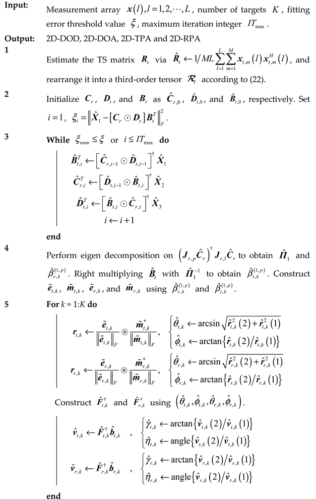
Algorithm 2: Algorithmic steps of the T-RS approach
Remotesensing 14 02905 i002
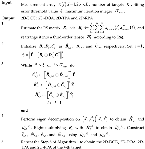
Algorithm 3: Algorithmic steps of the T-TRS approach
Remotesensing 14 02905 i003

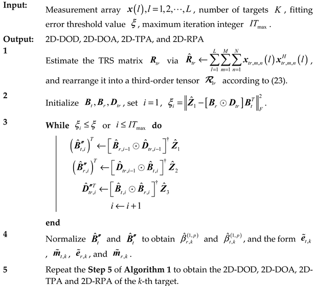
4. Algorithm Analysis

4.1. Complexity Analysis

The main complexities of the proposed estimators are the TALS for PARAFAC decomposition. For an M × N × L PARAFAC tensor with rank-K, the TALS procedure requires l [ M N L K + K 2 ( M L + N L + M N ) ] , where l represents the number of iterations required to achieve convergence. According to (22)–(24), the dimensions of the PARAFAC models associated with the T-TS approach, the T-RS approach, and the T-TRS approach are 6 × 6 N × 36 N , 6 M × 6 × 36 M , and 6 × 6 × 36 , respectively. Therefore, the main complexities of the T-TS approach, the T-RS approach, and the T-TRS approach are l [ 6 4 N 2 + 2 K 2 ( 6 3 N + 6 3 N 2 ) ] , l [ 6 4 M 2 + 2 K 2 ( 6 3 M + 6 3 M 2 ) ] , and l [ 6 4 + 6 3 K 2 ] , respectively. In comparison, the dominant complexity of the TS approach, the RS approach, and the TRS approach in [37] is the eigen decomposition of the covariance matrix. Accordingly, the dominant complexity of the TS approach, the RS approach, and the TRS approach are O { 36 3 N 3 } , O { 36 3 M 3 } , and O { 36 3 } , respectively. We list the main complexity comparison in Table 1. Notably, the main computational burden of the matrix-based approaches is on the third-order of the dimension of the covariance matrix, while the complexity may be lower in the tensor-based counterparts (since only the second-order of the Tx/Rx scale is involved), especially in the presence of large scale Tx/Rx EMVS array.

4.2. Identifiability Analysis

The identifiability (maximum K) is another important index to evaluate the estimator. The identifiability of a PARAFAC-model-based approach is usually constrained by the uniqueness condition of the PARAFAC condition, which is presented in (29). As a result, the uniqueness conditions with respect to T-TS, T-RS, and T-TRS are K 21 N + 2 , K 21 M + 2 , and K 23 , respectively. In Table 1, we list the identifiabilities of the proposed estimators. In addition, the identifiabilities corresponding to TS, RS, and TRS are added. It is observed from Table 1 that the proposed T-TS and T-RS methods have better identifiability than the matrix-based ones, while the T-TRS offers worse identifiability than the TRS approach.

4.3. CRB

The deterministic CRB on 2D-DOD, 2D-DOA, 2D-TPA, and 2D-TRA are given by [32]
C R B = σ 2 2 L [ Re { ( D ˜ H Γ C D ˜ ) ( R s 1 8 × 8 ) } ] 1
where D ˜ = [ c 1 θ t , 1 , , c K θ r , K , c 1 φ t , 1 , , c K η r , K ] 36 M N × 8 K with C = C t C r , c k denotes the k-th column of C ; Γ C = I M N C C ; denotes the Hadamard product; and 1 8 × 8 denotes the 8 × 8 matrix when all the entities are ones.

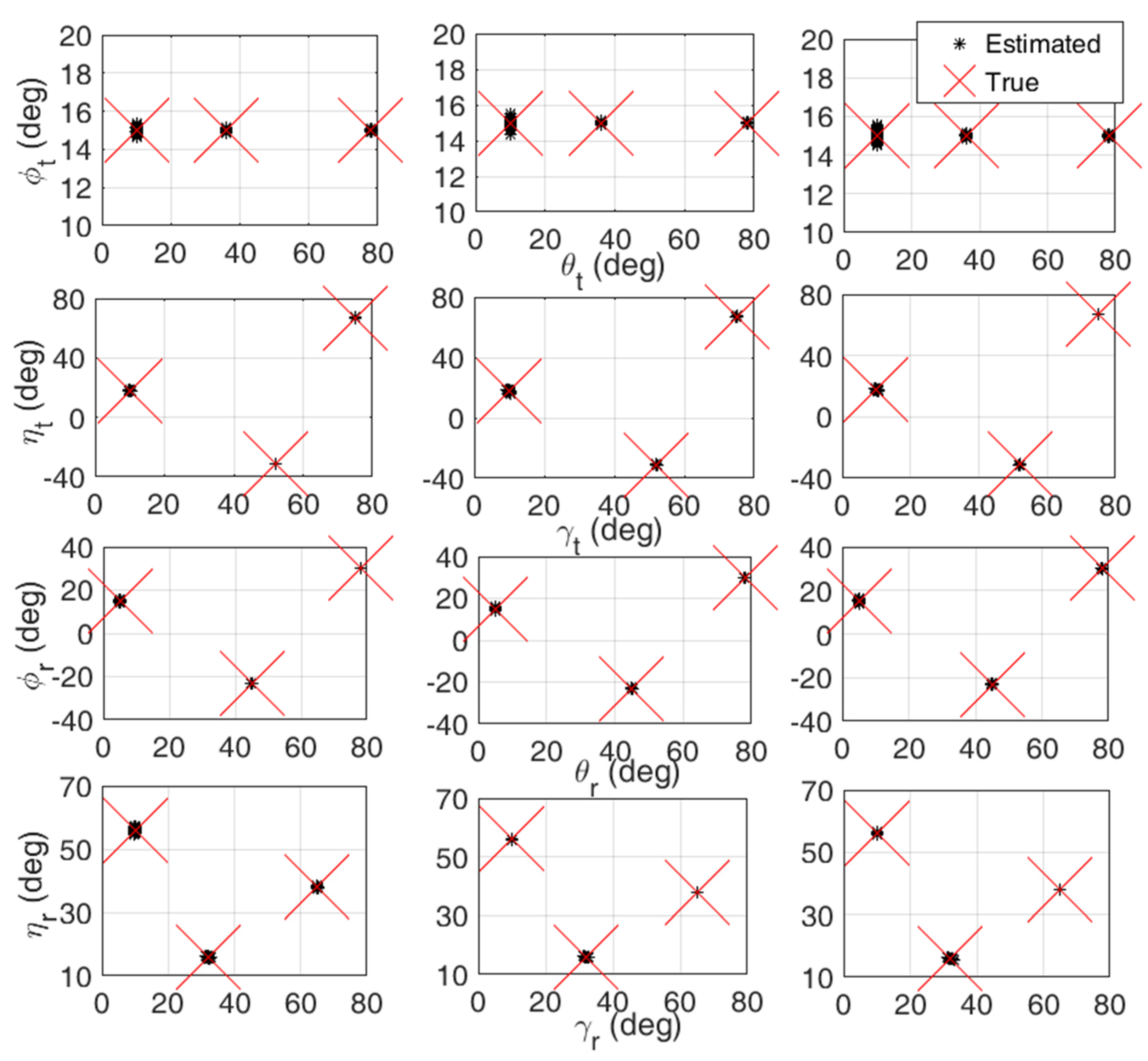
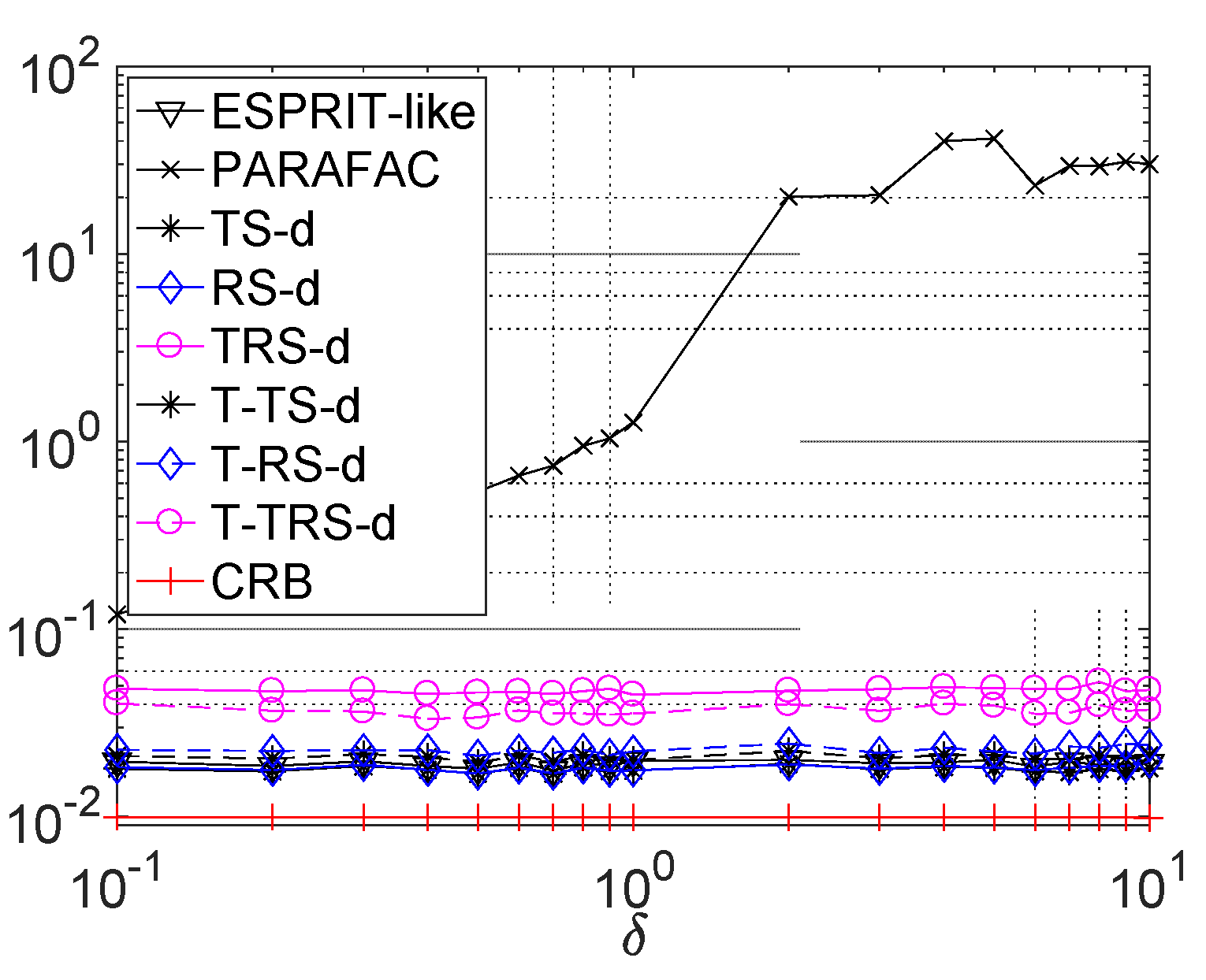
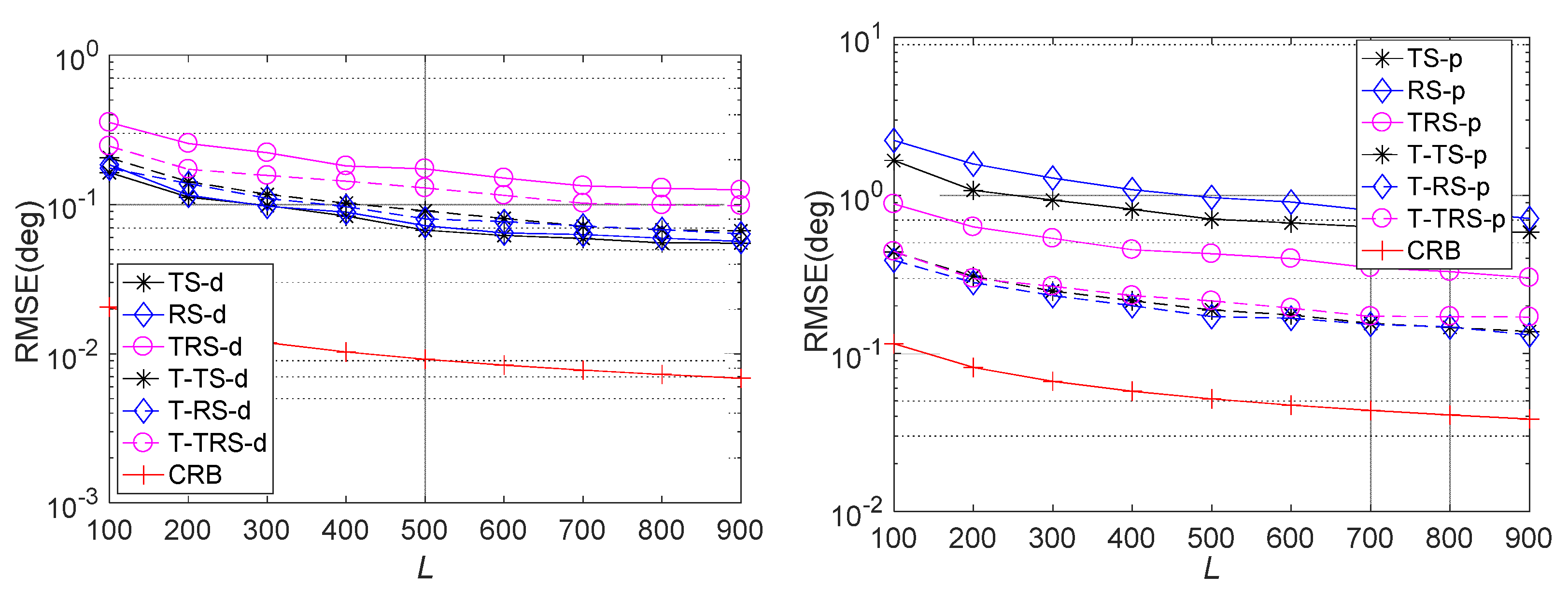
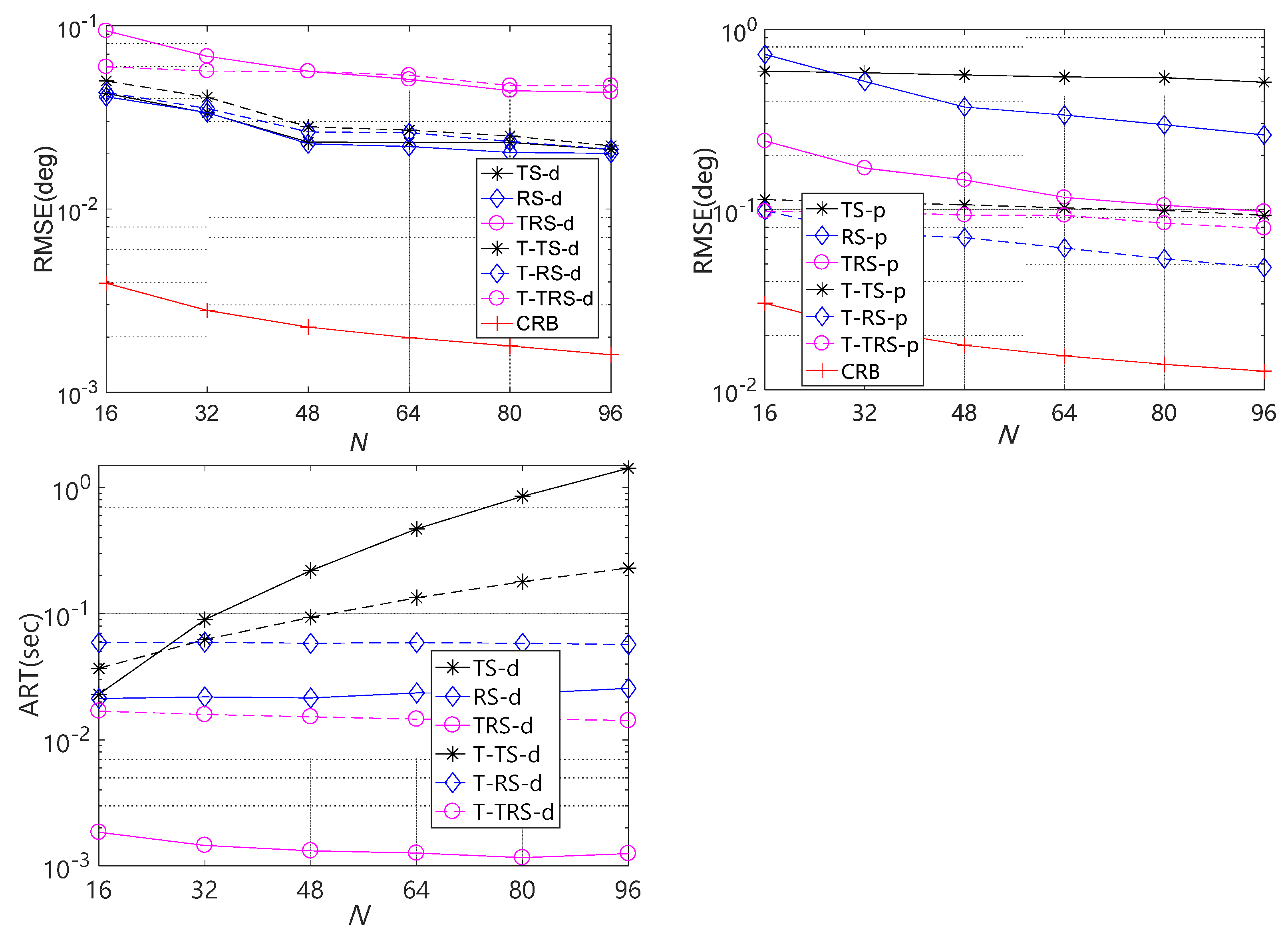
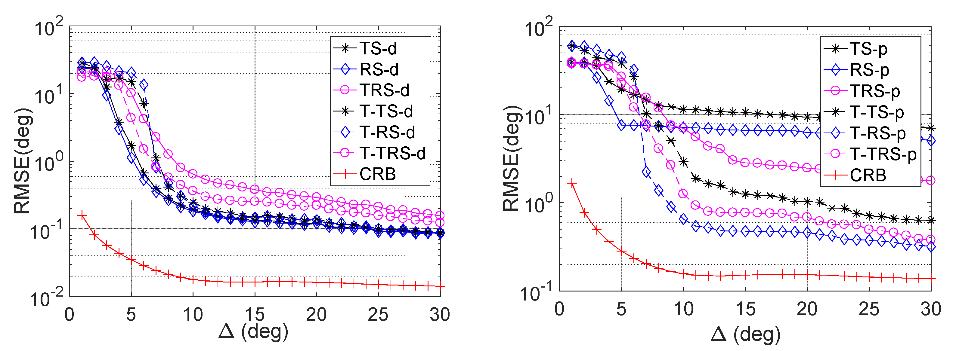
5. Simulation Results

In this section, Q = 200 Monte-Carlo trials are carried out to verify the effectiveness of our estimators. Suppose that there exist K far-field targets, and we assume that L snapshots are collected: the targets’ reflected coefficients satisfy a standard complex Gaussian distribution. Herein, we consider two different array configurations scenarios: Case (I) is the arbitrary geometries. The three-dimensional coordinates ( x t , m , y t , m , z t , m ) of each Tx sensor are randomly chosen from a uniform distribution u n i f ( κ t , κ t ) , while the three-dimensional coordinates ( x r , n , y r , n , z r , n ) of each Rx sensor are randomly chosen from another uniform distribution u n i f ( κ r , κ r ) . Case (II) is a ULA geometry. Both the Tx array and the Rx array are ULAs along the z-axis with half-wavelength spacing. Simulations are performed on a workstation with an Intel(R) Xeon(R) Silver 4214 CPU and 128 GB RAM, and MATLAB 2018b is adopted. The signal-to-noise ratio (SNR) is defined as the power ratio of x ( t ) n ( t ) to n ( t ) , and the two vectors are defined in (1). The estimation accuracy of the parameter ϑ is evaluated by the root mean square error (RMSE) defined as:
R M S E = 1 / Q q = 1 Q ( ϑ ^ q ϑ ) 2
where ϑ ^ q denotes the estimated ϑ in the q-th trial.
Example 1.
Scatter results of the proposed approaches. In Figure 2, we plot the scatter results of the proposed T-TS approach, the T-RS approach, as well as the T-TRS approach for completely coherent targets in Case (I). Herein, we consider K = 3 complete coherent targets with θ t = ( 10 ° , 36 ° , 78 ° ) , ϕ t = ( 15 ° , 15 ° , 15 ° ) , γ t = ( 10 ° , 52 ° , 75 ° ) , η t = ( 18 ° , 31 ° , 67 ° ) , θ r = ( 5 ° , 45 ° , 78 ° ) , ϕ r = ( 15 ° , 2 3 ° , 30 ° ) , γ r = ( 32 ° , 10 ° , 65 ° ) , and η r = ( 16 ° , 56 ° , 38 ° ) . Moreover, M = 8, N = 12, L = 500, κ t = 2 λ , κ r = 4 λ , and SNR = 0 dB are considered. It is obvious that 2D-DOD, 2D-DOA, 2D-TPA, and 2D-RPA can be accurately estimated by the T-TS, T-RS, and T-TRS approaches, and all the results are correctly paired. It is evident that the proposed approaches are effective for EMVS-MIMO radar, even through the two targets have the same Tx azimuth angle ϕ t .
Example 2.
RMSE of the proposed approaches versus SNR.Figure 3 gives the average RMSE on direction (2D-DOD and 2D-DOA) estimation and polarization (2D-TPA and 2D-RPA) estimation versus SNR comparison for K = 3 completely coherent targets in Case (I), where ϕ t = ( 15 ° , 50 ° , 53 ° ) , and other conditions are the same as in Example I. The average RMSE on direction and polarization are marked with suffixes ‘-d’ and ‘-p’, respectively. It is observed that all the approaches provide improved RMSE with the increasing SNR. Obviously, the TS approach and the RS approach offer more accuate direction estimations than the T-TS approach and the T-RS approach, while the proposed T-TRS approach achieves better estimation accuracy than the TRS approach. Interestingly, all the tensor-aware estimators offer much better polarization estimation accuracy than their matrix counterparts. In addition, it should be noticed that there are gaps between all the mentioned approaches and the CRB, implying that there is room to further improve the estimation accuracy.
Example 3.
RMSE comparisons of various algorithms with ULA geometry. Herein, the performances with respect to the PARAFAC estimator in [32] and the ESPRIT-like algorithm in [34] are added. Unless otherwise specified, the simulation conditions are the same as in Example 2. Figure 4 (upper left) displays the average RMSE on direction estimation versus the SNR, from which we can observe that both ESPRIT-like and traditional PARAFAC algorithms fail to work in the presence of coherent targets. In addition, the tensor-based smoothing approaches outperform the matrix-based ones. Figure 4 (upper right) presents the average RMSE versus correlation coefficient between targets, where the SNR is set to 10 dB. As expected, both ESPRIT-like and traditional PARAFAC algorithms have very close (or even better) RMSE performances to the smoothing approaches. However, they would achieve decreased RMSE with the increasing α once α is larger than a given threshold. However, RMSE of the smoothing-based approaches barely change during the entire α regions. Figure 4 (lower left) shows the RMSE results of various estimators versus sensor position error factor δ, where random position error unif ([0, δλ]) is considered in both the Tx and Rx arrays, and the SNR is set to 20 dB. Obvious, the RMSE of all the estimators barely change with δ, except the traditional PARAFAC algorithm. It is evident that the proposed estimators are insensitive to sensor position errors.
Example 4.
RMSE comparisons versus snapshot L in case (I).Figure 5 presents the average RMSE on direction estimation and polarization estimation at different snapshot numbers L in Case (I), where the SNR is fixed at 10 dB and other conditions are the same as in Example 2. The observations in Figure 5 are similar to that in Figure 3. The proposed tensor-based approaches achieve better RMSE than the matrix-based approaches in polarization parameter estimation, but they may perform worse than the latter in direction parameter estimation.
Example 5.
Performance comparisons versus Rx EMVS number N in case (I).Figure 6 illustrates the average RMSE comparison and average running time (ART) comparison for completely coherent targets in Case (I) with different Rx EMVS number N, where M = 12, κ t = 2 λ , κ r = 16 λ , L = 500, and SNR = 10 dB are considered. In such a configuration, the MIMO radar system can be interpreted as a massive MIMO radar since there are 72 Tx components and 6N Rx components. It is shown that the tensor approaches offer a much closer direction estimation performance than the matrix approaches, and they outperform the matrix counterparts with respect to polarization parameter estimation. As expected, the T-TS approach is much more efficient than the TS approach, especially in the presence of large N. However, since M is relatively small, the T-RS approach and the T-TRS approach would require more calculation time than the RS approach and the TRS approach, respectively. In sum, there is a trade-off between running time and the estimation accuracy. In practice, the approprite algorithm should be chosen to balance the two indices.
Example 6.
RMSE comparison versus target distance in case (I).Figure 7 illustrates the average RMSE comparison for completely coherent targets in Case (I) with different inter-target distance Δ , where K = 2 complete coherent targets are considered with parameters θ t = ( 10 ° , 10 ° + Δ ) , ϕ t = ( 15 ° , 15 ° + Δ ) , γ t = ( 10 ° , 10 ° + Δ ) , η t = ( 16 ° , 16 ° + Δ ) , θ r = ( 12 ° , 12 ° + Δ ) , ϕ r = ( 11 ° , 11 ° + Δ ) , γ r = ( 2 ° , 2 ° + Δ ) and η r = ( 7 ° , 7 ° + Δ ) . Moreover, for L = 200 and SNR = 10 dB, other conditions are the same as in Example 1. It is observed that the RMSE of all the methods will improved quickly with the increasing Δ when Δ is smaller than 10 ; otherwise the RMSE of all the methods would be improved slowly with the increasing Δ . Since the proposed approaches can take advantage of the tensor nature, they outperform the matrix-based estimators, especially in polarization parameters estimation.

6. Conclusions

In this paper, three estimators based on PARAFAC decomposition are introduced for 2D-DOD, 2D-DOA, 2D-TPA, and 2D-RPA estimation in a bistatic EMVS-MIMO radar with coherent targets. The core idea of the proposed estimators is to de-correlate the coherent targets via spatial smoothing and then formulate the covariance matrix into a third-order PARAFAC decomposition model. After performing PARAFAC decomposition, the factor matrices with respect to various PARAFAC models are obtained. Then, the 2D-DOD and 2D-DOA are achieved via the normalized vector cross-product technique. Finally, the 2D-TPA and 2D-RPA are estimated via the LS technique. Simulations coincide with the theorical results. In the near future, attention should be paid to developing more effective estimation algorithms.

Author Contributions

Conceptualization, L.Z. and H.W.; methodology, F.-Q.W. and J.-P.S.; All authors have read and agreed to the published version of the manuscript.

Funding

This work is supported by China NSF Grants (62071476) and partly supported by Shaanxi Provincial Key R&D Plan (No. 2020SF-166).

Data Availability Statement

Not applicable.

Conflicts of Interest

The authors declare no conflict of interest.

References

  1. Fisher, E.; Haimovich, A.; Blum, R.; Ciminio, L.; Chizhik, D. MIMO radar: An idea whose time has come. In Proceedings of the 2004 IEEE Radar Conference (IEEE Cat. No. 04CH37509), Philadelphia, PA, USA, 29 April 2004; pp. 71–78. [Google Scholar]
  2. Zhang, L.; Wen, F. A novel MIMO radar orthogonal waveform design algorithm based on intelligent ions motion. Remote Sens. 2021, 13, 1968. [Google Scholar] [CrossRef]
  3. Shi, J.; Yang, Z.; Liu, Y. On parameter identifiability of diversity-smoothing-based MIMO radar. IEEE Trans. Aerosp. Electron. Syst. 2022, 58, 1660–1675. [Google Scholar] [CrossRef]
  4. Li, J.; Stoica, P. MIMO radar with colocated antennas. IEEE Signal Process Mag. 2007, 24, 106–114. [Google Scholar] [CrossRef]
  5. Chen, D.; Chen, B.; Qin, G. Angle estimation using ESPRIT in MIMO radar. Electron. Lett. 2008, 44, 770–771. [Google Scholar]
  6. Chen, J.; Gu, H.; Su, W. Angle estimation using ESPRIT without pairing in MIMO radar. Electron. Lett. 2008, 44, 1422–1423. [Google Scholar]
  7. Yan, H.; Li, J.; Liao, G. Multitarget identification and localization using bistatic MIMO radar systems. EURASIP J. Adv. Signal Process. 2008, 48, 1–8. [Google Scholar] [CrossRef] [Green Version]
  8. Zhang, X.; Xu, L.; Lei, X.; Xu, D. Direction of departure (DOD) and direction of arrival (DOA) estimation in MIMO radar with reduced-dimension MUSIC. IEEE Commun. Lett. 2010, 14, 1161–1163. [Google Scholar] [CrossRef]
  9. Xu, D.; Zhang, X.; Huang, Y.; Chen, C.; Li, J. Reduced-complexity Capon for direction of arrival estimation in a monostatic multiple-input multiple-output radar. IET Radar Sonar Nav. 2012, 6, 796–801. [Google Scholar]
  10. Zhang, X.; Xu, Z.; Xu, L.; Xu, D. Trilinear decomposition-based transmit angle and receive angle estimation for multiple-input multiple-output radar. IET Radar Sonar Nav. 2011, 5, 626–631. [Google Scholar] [CrossRef]
  11. Cheng, Y.; Yu, R.; Gu, H.; Su, W. Multi-SVD based subspace estimation to improve angle estimation accuracy in bistatic MIMO radar. Signal Process. 2013, 93, 2003–2009. [Google Scholar] [CrossRef]
  12. Wang, Z.; Cai, C.; Wen, F.; Huang, D. A quadrilinear decomposition method for direction estimation in bistatic MIMO radar. IEEE ACCESS 2018, 6, 18451–18458. [Google Scholar] [CrossRef]
  13. Guo, Y.; Wang, X.; Lan, X.; Su, T. Traffic target location estimation based on tensor decomposition in intelligent transportation system. IEEE Trans. Intell. Transp. Syst. 2022, 1–13. [Google Scholar] [CrossRef]
  14. Liu, W.; Liu, J.; Hao, P.; Gao, Y.; Wang, G.; Wang, Y. Multichannel signal detection in interference and noise when signal mismatch happens. Signal Process. 2020, 166, 107268. [Google Scholar] [CrossRef]
  15. Wu, J.; Wen, F.; Shi, J. Direction finding in bistatic MIMO radar with direction-dependent mutual coupling. IEEE Commun. Lett. 2021, 25, 2231–2234. [Google Scholar] [CrossRef]
  16. Wu, J.; Wen, F.; Shi, J. Fast angle estimation in MIMO system with direction-dependent mutual coupling. IEEE Commun. Lett. 2021, 25, 2913–2917. [Google Scholar] [CrossRef]
  17. Liu, W.; Liu, J.; Hao, P.; Gao, Y.; Wang, Y. Multichannel adaptive signal detection: Basic theory and literature review. Sci. China Inform. Sci. 2022, 65, 121301. [Google Scholar] [CrossRef]
  18. Wang, H.; Xiao, P.; Li, X. Channel parameter estimation of mmWave MIMO system in urban traffic scene: A training channel based method. IEEE Trans. Intell. Transp. Syst. 2022, 1–9. [Google Scholar] [CrossRef]
  19. Li, J.; Li, P.; Tang, L.; Zhang, X.; Wu, Q. Self-Position awareness based on cascade direct localization over multiple source data. IEEE Trans. Intell. Transp. Syst. 2022, 1–9. [Google Scholar] [CrossRef]
  20. Chen, C.; Zhang, X. A low-complexity joint 2D-DOD and 2D-DOA estimation algorithm for MIMO radar with arbitrary arrays. Int. J. Electron. 2013, 100, 1455–1469. [Google Scholar] [CrossRef]
  21. Li, J.; Zhang, X. Closed-form blind 2D-DOD and 2D-DOA estimation for MIMO radar with arbitrary arrays. Wirel. Per. Commun. 2013, 69, 175–186. [Google Scholar] [CrossRef]
  22. Xia, T. Joint diagonalization based 2D-DOD and 2D-DOA estimation for bistatic MIMO radar. Signal Process. 2015, 116, 7–12. [Google Scholar] [CrossRef]
  23. Serio, A.D.; Hugler, P.; Roos, F.; Waldschmidt, C. 2D-MIMO radar: A method for array performance assessment and design of a planar antenna array. IEEE Trans. Antenn. Propag. 2020, 68, 4604–4616. [Google Scholar] [CrossRef]
  24. Wen, F.; Shi, J.; Wang, X.; Wang, L. Angle estimation for MIMO radar in the presence of gain-phase errors with one instrumental Tx/Rx sensor: A theoretical and numerical study. Remote Sens. 2021, 13, 2964. [Google Scholar] [CrossRef]
  25. He, J.; Shu, T.; Li, L.; Truong, T.K. Mixed near-field and far-field localization and array calibration with partly calibrated arrays. IEEE Trans. Signal Process. 2022, 70, 2105–2118. [Google Scholar] [CrossRef]
  26. Wong, K.T.; Yuan, X. “Vector cross-product direction-finding” with an electromagnetic vector-sensor of six orthogonally oriented but spatially noncollocating dipoles/loops. IEEE Trans. Signal Process. 2011, 59, 160–171. [Google Scholar] [CrossRef]
  27. Tanveer, A.; Zhang, X.; Zheng, W. DOA estimation for coprime EMVS arrays via minimum distance criterion based on PARAFAC analysis. IET Radar Sonar Nav. 2019, 13, 65–73. [Google Scholar]
  28. Zheng, G.; Song, Y.; Chen, C. Height measurement with meter wave polarimetric MIMO radar: Signal model and MUSIC-like algorithm. Signal Process. 2022, 190, 108344. [Google Scholar] [CrossRef]
  29. Shu, T.; He, J.; Dakulagi, V. 3-D near-field source localization using a spatially spread acoustic vector sensor. IEEE Trans. Aerosp. Electron. Syst. 2022, 58, 180–188. [Google Scholar] [CrossRef]
  30. Chintagunta, S.; Palanisamy, P. 2D-DOD and 2D-DOA estimation using the electromagnetic vector sensors. Signal Process. 2018, 147, 163–172. [Google Scholar] [CrossRef]
  31. Wen, F.; Shi, J. Fast direction finding for bistatic EMVS-MIMO radar without pairing. Signal Process. 2020, 173, 107512. [Google Scholar] [CrossRef]
  32. Wen, F.; Shi, J.; Zhang, Z. Joint 2D-DOD, 2D-DOA, and polarization angles estimation for bistatic EMVS-MIMO radar via PARAFAC analysis. IEEE Trans. Veh. Technol. 2020, 69, 1626–1638. [Google Scholar] [CrossRef]
  33. Wang, X.; Huang, M.; Wan, L. Joint 2D-DOD and 2D-DOA estimation for coprime EMVS-MIMO radar. Circ. Syst. Signal Process. 2021, 40, 2950–2966. [Google Scholar] [CrossRef]
  34. Wen, F.; Shi, J.; Zhang, Z. Closed-form estimation algorithm for EMVS-MIMO radar with arbitrary sensor geometry. Signal Process. 2021, 186, 108117. [Google Scholar] [CrossRef]
  35. Ponnusamy, P.; Subramaniam, K.; Chintagunta, S. Computationally efficient method for joint DOD and DOA estimation of coherent targets in MIMO radar. Signal Process. 2019, 165, 262–267. [Google Scholar] [CrossRef]
  36. Chintagunta, S.; Ponnusamy, P.; Subramaniam, K. Polarization difference smoothing in bistatic MIMO radar. Prog. Electromagn. Res. Lett. 2020, 88, 67–74. [Google Scholar]
  37. Wen, F.; Shi, J.; Zhang, Z. Generalized spatial smoothing in bistatic EMVS-MIMO radar. Signal Process. 2022, 193, 108406. [Google Scholar] [CrossRef]
  38. Kolda, T.G.; Bader, B.W. Tensor Decompositions and Applications. SIAM Rev. 2009, 51, 455–500. [Google Scholar] [CrossRef]
  39. Rao, W.; Li, D.; Zhang, J.Q. A Tensor-Based Approach to L-Shaped Arrays Processing with Enhanced Degrees of Freedom. IEEE Signal. Process. Lett. 2018, 25, 234–238. [Google Scholar] [CrossRef]
  40. Chen, Y.H. On spatial smoothing for two-dimensional direction-of-arrival estimation of coherent signals. IEEE Trans. Signal Process. 1997, 45, 1689–1696. [Google Scholar] [CrossRef] [Green Version]
  41. Bro, R.; Sidiropoulos, N.; Giannakis, G. A Fast Least Squares Algorithm for Separating Trilinear Mixtures. In Proceedings of the International Workshop ICA and BSS, Aussois, France, 11–15 January 1999; pp. 289–294. [Google Scholar]
Figure 1. Schematic diagram of the bistatic EMVS-MIMO radar with arbitrary geometry.
Remotesensing 14 02905 g001
Figure 2. Scatter results of the proposed approaches for complete coherent targets in Case (I). (left) T-TS approach, (Middle) T-RS approach, and (Right) T-TRS approach.
Remotesensing 14 02905 g002
Figure 3. RMSE of parameter estimation versus SNR in Case (I).
Remotesensing 14 02905 g003
Figure 4. RMSE comparison in Case (II). (upper left) RMSE versus SNR comparison; (upper right) RMSE versus target correlation coefficient α; (lower left) RMSE versus sensor position error factor δ.
Remotesensing 14 02905 g004aRemotesensing 14 02905 g004b
Figure 5. RMSE of parameters estimation versus L in Case (I).
Remotesensing 14 02905 g005
Figure 6. RMSE and ART comparisons versus N in Case (I).
Remotesensing 14 02905 g006
Figure 7. RMSE comparisons versus target distance Δ in Case (I).
Remotesensing 14 02905 g007
Table 1. Complexity and identifiability comparison.
AlgorithmComputing ComplexityIdentifiability
TS O { 36 3 N 3 } 6 N
RS O { 36 3 M 3 } 6 M
TRS O { 36 3 } 36
T-TS l [ 6 4 N 2 + 2 K 2 ( 6 3 N + 6 3 N 2 ) ] 21 N + 2
T-RS l [ 6 4 M 2 + 2 K 2 ( 6 3 M + 6 3 M 2 ) ] 21 M + 2
T-TRS l [ 6 4 + 6 3 K 2 ] 23
Publisher’s Note: MDPI stays neutral with regard to jurisdictional claims in published maps and institutional affiliations.

