Abstract
Ecological changes affected by increasing human activities have highlighted the importance of ecological quality assessments. An appropriate and efficient selection of ecological parameters is fundamental for ecological quality assessments. On the basis of remote sensing data and methods, this study developed an enhanced ecological evaluation index (EEEI) with five integrated ecological parameters by containing pixel and sub-pixel information: normalized difference vegetation index, impervious surface coverage, soil coverage, land surface temperature, and wetness component of tasseled cap transformation. Significantly, the EEEI simultaneously considered the five aspects of land surface ecological conditions (i.e., greenness, human activities, dryness, heat, and moisture), which provided an effective guide for the systematic selection of ecological parameters. The EEEI has a clear theoretical framework, and all the parameters can be obtained quickly on the basis of the remote sensing datasets and methods, which is suitable for the promotion and application of ecological quality assessments to various areas and scales. Furthermore, the EEEI was applied to assess and detect the ecological quality of the Guangdong–Hong Kong–Macau Greater Bay Area (GBA) of China. Assessment results indicated that the ecological quality of the GBA is currently facing great challenges with a degradation trend from 2000 to 2020, which emphasizes the significance and urgency for eco-environmental protection of the GBA. This provided evidence that the EEEI can be used as an effective index for scientific, objective, quantitative, and comprehensive ecological quality assessment, which can also aid regional environmental management and ecological protection.
1. Introduction
Under the continuous development of global climate change and anthropogenic disturbances, global and local ecosystems have been significantly altered more than ever before [1,2,3,4,5]. The increase of human activities has led to dramatic land cover changes from natural landscapes to built-up areas [6,7,8,9,10]. From this change, a range of negative ecological environmental impacts also occur, such as deterioration of water quality [11,12], urban heat islands [13,14,15], urban waterlogging [16,17], and biodiversity reduction [18,19]. Therefore, it is increasingly necessary to assess and monitor ecological states and spatiotemporal changes to provide scientific knowledge for the guidance of eco-environmental management and sustainable development for local and global regions.
Advances in remote sensing technologies and resources provide potential opportunities for rapidly and effectively monitoring various scales of ecological quality. Remote sensing images, with the advantage of large-areal, fast, real-time, and cyclical repeat observations, are commonly applied for ecological quality monitoring. Many remote sensing parameters and indices, such as the normalized difference vegetation index (NDVI), land surface temperature (LST), or impervious surface area, have been applied for ecological quality assessments [20,21,22,23,24,25]. However, applications with a single ecological parameter or index have difficulties in revealing a comprehensive ecological quality assessment.
The most critical step of a remotely sensed ecological quality evaluation is to select the suitable parameters related to the eco-environment by utilizing remote sensing data and methods. Based on the purpose of comprehensive ecological quality assessments, scholars have designed a series of ecological indices that integrate several remotely sensed parameters (Table 1). Significantly, Xu [26] proposed a remote sensing ecological index (RSEI) for the assessment of ecological quality that integrates four ecological factors: green, wetness, dryness, and temperature. Four remote sensing parameters, namely, NDVI, wetness component of tasseled cap transformation (TCT) (WET), normalized differential build-up and bare soil index (NDBSI), and LST, were selected to represent the four ecological factors. Next, principal components analysis (PCA) regression was used to integrate the four parameters for a synthetic index (RSEI). Many studies have proven that the RSEI can make a rapid and comprehensive evaluation of ecological quality at various scales, such as nationwide or provincial region [27,28], urban agglomeration [29], urban or county region [30,31,32], mining area [33], and wetland or lake basin [34,35]. The results of ecological quality evaluated by the RESI can be visualized in both spatial and temporal ways, which has practical significance with high credibility.

Table 1.
Representative studies of ecological assessment based on multiple remotely sensed parameters.
Some scholars tried to improve the ecological indices by changing parameter selection and the number of principal components. For example, Yang et al. [29] proposed a comprehensive ecological quality evaluation index, where vegetation cover and vegetation health index were used to replace NDVI parameters. Wang et al. [36] offered the arid RSEI, which was integrated with five ecological factors, namely, greenness, humidity, heat, salinity, and land degradation, to evaluate the ecological quality of arid regions. Song et al. [37] used the first and second principal components to construct the modified RSEI. Additionally, new ecological indices have continually been proposed on the basis of remote sensing data for local ecological quality assessments. He et al. [38] developed a comprehensive evaluation index containing fine particulate matter (PM2.5) data, LST, and vegetation cover (VC) to evaluate the urban environmental change in China. Firozjaei et al. [39] presented a remotely sensed urban surface ecological index by taking the imperviousness data product from the National Land Cover Database as one of the ecological parameters to assess the surface ecological conditions in different urban environments. These studies greatly support ecological quality evaluations based on remote sensing technology.
Furthermore, the integration of different parameters is another key issue of ecological quality evaluation. PCA regression [26,29] and linear combination [40,41] are widely used methods for parameter integration. In practice, it is difficult for linear combination to determine the weights of different parameters, which is most likely affected by subjective experience. PCA can remove the impacts of co-linearity between the four parameters [42], and the weight of each parameter is objectively and automatically allocated by each parameter’s contribution to the principal components. Thus, the errors or divergences in weight definition due to the subjective characteristics can be mostly prevented. Therefore, PCA has more advantages in applications of parameter integration.
An appropriate selection of ecological parameters is fundamental for the evaluation of ecological quality. However, previous studies focused on different dimensions of ecological quality using diverse parameters that lacked a comprehensively systematic model to provide an effective ecological evaluation. Therefore, how to organize and enhance ecological parameter selection has become an imperative and challenging research topic for ecological quality assessments. Firstly, the NDVI is widely used to assess vegetation cover at different scales, which has a positive effect on ecological quality. Compared with other vegetation factors, the NDVI has the most direct and convenient reflections of land surface greenness [42]. Secondly, the LST and WET are important factors of local climate, respectively, supplying heat and moisture for land surface ecosystems [43]. Furthermore, soil coverage (SC) represents regions with sparsely vegetated coverage, which can be used to indicate land surface dryness [44]. Additionally, the impervious surface coverage (ISC) represents the impact of human activities and has increasingly been considered as an important environmental indicator [45,46,47]. The ISC can be used as an effective factor to quantify the effects of human activities on land surface ecosystems. These five factors (NDVI, ISC, SC, LST, and WET) are key to the eco-environment evaluation of land surfaces, which directly reflect ecological qualities from greenness, human activities, dryness, heat, and moisture. Therefore, the integrated information of these five factors can effectively and comprehensively reveal the ecological quality of land surfaces.
This study provides a guidance for ecological quality evaluations of land surfaces from remote sensing and helps select suitable parameters for an objective, quantitative, and comprehensive assessment of ecological quality. To achieve this goal, this study developed an enhanced ecological evaluation index (EEEI) integrated with five ecological parameters (NDVI, ISC, SC, LST, and WET) by containing pixel and sub-pixel information. Specifically, we aimed to (1) develop the EEEI on the basis of the five ecological parameters; (2) analyze the capability and performance of the EEEI; and (3) provide a case study of a spatiotemporal ecological quality assessment in the Guangdong–Hong Kong–Macau Greater Bay Area (GBA) of China from 2000 to 2020. This study helps with the systematic selection of ecological parameters for an efficient ecological quality assessment, which can also contribute to regional environmental management, ecological protection, and sustainable development.
2. Development of the EEEI
The development of the EEEI contained two key steps, selection of the parameters and integration of the EEEI. The five ecological parameters (NDVI, ISC, SC, LST, and WET) represent land surface ecological qualities from greenness, human activities, dryness, heat, and moisture. The ecological meaning of the five parameters was shown in Table 2. Then, the PCA regression was adopted to develop a synthetic index (EEEI). The methodological framework of this research is presented in Figure 1. The theoretical framework of the EEEI, calculation of five ecological parameters, and integration of the EEEI are described in the following sections.
Table 2.
The ecological meaning of the five parameters.
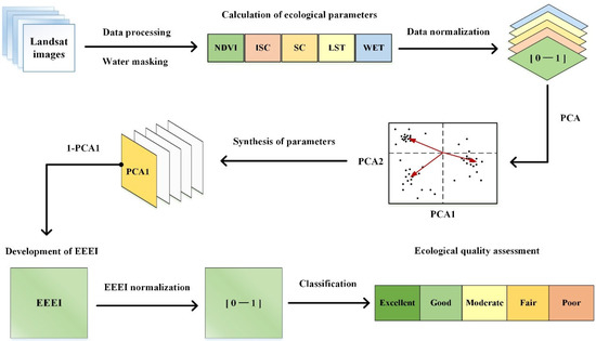
Figure 1.
The methodological framework. NDVI: normalized difference vegetation index; ISC: impervious surface coverage; SC: soil coverage; LST: land surface temperature; WET: wetness component of tasseled cap transformation; PCA: principal components analysis; EEEI: enhanced ecological evaluation index.
2.1. Theoretical Framework of EEEI
The EEEI was proposed to assess the ecological quality by integrating five remote sensing-based ecological parameters (NDVI, ISC, SC, LST, and WET). These parameters were elaborately selected with pressure–state–response framework, which was constructed on the measurement and analysis of anthropogenic pressure, eco-environmental status, and climate response as parameters [48]. The ecological parameters in EEEI were selected based on previous studies [28,29,49]. Firstly, ecological conditions and processes within a certain range are typically affected by dynamic changes in land use/cover change to a large extent. Among them, the most significant feature is the change from natural landscape into construction under the pressure of anthropogenic activities. Therefore, the ISC can be used to indicate the intensity of anthropogenic pressures on ecological conditions. Secondly, the indicators of ecological states are designed to represent the environmental background and the quantity and quality of resources. Hence, the NDVI and the SC, respectively, representing the greenness and dryness, were selected to describe the ecological state. Finally, the LST and the WET were utilized to indicate comprehensive climate (temperature and humidity) changes in response to ecological changes. Therefore, the EEEI integrated with the five ecological parameters can be used as an effective index for ecological evaluation.
2.2. Calculation of Ecological Parameters
- NDVI;
The NDVI was calculated as follows:
where and represent the near infrared red band and red band of the images, respectively.
- 2.
- ISC and SC;
The ISC and the SC were calculated by linear spectral mixture analysis (LSMA) under a four-end-member model (vegetation, high-albedo impervious surface, low-albedo impervious surface, and soil) in this study [50].
The LSMA method decomposes the spectrum of each pixel into different proportions at the sub-pixel level [51,52], which can be expressed as follows:
where is number of spectral bands; = 1, …, n (number of endmembers); is the spectral reflectance of band ; is the proportion of endmembers in the pixel; is the spectral reflectance of endmember in band ; and is the estimating error for band . The above equation must satisfy the following restrictions:
The ISC and the SC with a value range of 0 to 1 were obtained by the LSMA method at the sub-pixel level. To obtain more accurate results of the ISC and the SC, three spectral indices made by setting up appropriate thresholds were used to optimize the initial unmixing results. Firstly, the NDVI (Equation (1)) was used to remove the vegetation from the impervious surface fraction and the soil fraction. Secondly, the normalized different build-up index (NDBI) (Equation (4)) [53] was selected to eliminate the impervious surface from the soil fraction. Lastly, the normalized different bare soil index (NDBaI) (Equation (5)) [44] was applied to eliminate the soil from the impervious surface fraction. The equations are as follows:
where , , and represents the near infrared red band, shortwave infrared red band, and thermal band of the images, respectively.
Additionally, the appropriate thresholds of each spectral index needed to be determined. Google Earth images with 1 m spatial resolution were used as the reference maps. Taking the NDVI as an example, 300 samples of pure vegetation pixels were selected from the study area. Next, the value ranges of the NDVI were obtained, and the average value was considered as the threshold value of NDVI. Analogously, the thresholds of NDBI and NDBaI were determined from the above steps. In this study, the thresholds of the NDVI, NDBI, and NDBaI were set as 0.7, 0, and 0, respectively (Figure 2).
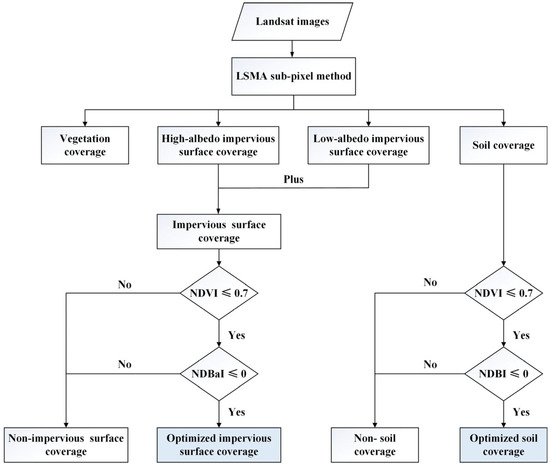
Figure 2.
The processing steps for calculation of the impervious surface coverage and the soil coverage. LSMA: linear spectral mixture analysis; NDVI: normalized difference vegetation index; NDBI: normalized different build-up index; and NDBaI: normalized different bare soil index.
- 3.
- LST;
The LST can be retrieved in the User’s Handbook of Landsat Data (http://landsathandbook.gsfc.nasa.gov/, accessed on 13 January 2021) and the coefficients of radiometric calibration [54,55]. The thermal bands of Landsat images (band 6 of Landsat TM and band 10 of Landsat OLI) were used to retrieve the LST in the following equations:
where is the spectral radiance values of the thermal band; is the values of the thermal band; and are gain and bias values of the thermal band, respectively; represents the at-satellite brightness temperature of the thermal band; and and are pre-launch calibration constants, which can be obtained from the User’s Handbook of Landsat Data.
where is the surface emissivity; represents the center wavelength () of the thermal band; the value is 1.438 (mK); means the VC; and in this study, the and values are 0% and 70%, respectively.
- 4.
- WET;
The WET was obtained from the wetness component of TCT in this study [26]. The calculation of the WET model is different for Landsat TM and Landsat OLI images.
where , , , , , and are the blue, green, red, near infrared red, shortwave infrared red band 1, shortwave infrared red band 2 of the Landsat image, respectively.
- 5.
- Data normalization.
As the ecological parameters have different dimensions, the NDVI, the LST, and the WET parameters were rescaled from 0 to 1. The equation of normalization is as follows:
where is the normalized value of one of the parameters and and are the minimum and maximum values of one of the parameters, respectively.
2.3. Integration of the EEEI
Five normalized ecological parameters were obtained by the above methods. Therefore, the key to this study is how to design a comprehensive ecological index that can integrate the information of the five parameters. The PCA regression was adopted to develop a synthetic index (EEEI). PCA is one of the compression technologies for multi-dimensional data that can eliminate the effects of co-linearity among different variables [26,42]. Additionally, the weight of each variable can objectively and automatically be allocated based on the contribution of each variable to the principal components. By this means, the errors or variations in weight assignment caused by subjective factors can be avoided. PCA was utilized for identifying the relative importance of these variables, and thus the weights of these variables were considered to be robust.
Firstly, PCA was used to integrate the five ecological parameters, and then the first component of PCA (PCA1) image was utilized to create the EEEI image, which contains the most information of all parameters. Finally, to make the larger values represent better ecological quality, the values of the PCA1 image were subtracted by 1.
The EEEI can be expressed as follows:
Finally, the values of the EEEI image were normalized from 0 to 1 so the ecological quality can be compared among the different study periods and regions. Therefore, the higher the EEEI value, the better the ecological quality, and vice versa.
3. Study Area and Datasets
3.1. Study Area
As a case study, we conducted a spatiotemporal ecological quality assessment in the GBA region of China from 2000 to 2020. The GBA lies on the southern coast of China and covers a total area of approximately 56,000 km2, with a total permanent population of more than 70 million (2020), including 11 cities (i.e., Guangzhou, Shenzhen, Foshan, Zhongshan, Zhuhai, Jiangmen, Zhaoqing, Dongguan, Huizhou, Hong Kong, and Macau) (Figure 3).
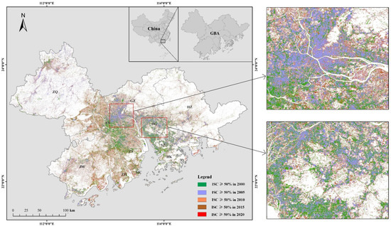
Figure 3.
Location of the GBA and the expansion of impervious surface from 2000 to 2020. GBA: Guangdong–Hong Kong–Macau Greater Bay Area, GZ: Guangzhou, SZ: Shenzhen, FS: Foshan, ZS: Zhongshan, ZH: Zhuhai, JM: Jiangmen, ZQ: Zhaoqing, DG: Dongguan, HZ: Huizhou, HK: Hong Kong, MC: Macau, ISC: impervious surface coverage.
The GBA is one of the major bay areas in the world. Given its location with a long coastline and the policy of “reform and open-up,” the area has gradually become the forefront of rapid development and urbanization in China. With the increasing urbanization rates, the impervious surfaces of the GBA are continuously expanding (Figure 3). Thus, the ecological conditions of the GBA have been affected by economic construction and anthropogenic activities. Therefore, it is urgent to conduct ecological evaluations to understand the ecological environment and its spatiotemporal evolution in the GBA.
3.2. Data Resources and Pre-Processing
The GBA is covered by eight Landsat images (Table 3). The Landsat images were selected from the United States Geological Survey (https://www.usgs.gov/, accessed on 4 January 2021) platform, including 24 Landsat TM images and 16 Landsat OLI images. All images are of good quality, with less than 10% cloud cover. The radiometric calibrations and the atmospheric corrections of these images were completed before the calculation of ecological parameters. Additionally, the water body pixels of each image were masked out through the modified normalized difference water index [56].
Table 3.
Information of Landsat images used in this study.
4. Results and Analysis
4.1. Capability and Performance of the EEEI
The five ecological parameters were integrated by PCA, and the PCA1-band image was selected to develop the EEEI image of the GBA from 2000 to 2020. As shown in Table 4, the eigen percentages of PCA1 are higher than 78% for the study years, which indicates that it represents the primary information and characteristics of the dataset. Therefore, the EEEI created by PCA1 can effectively contain most of the information of the five parameters. Moreover, the correlation among the EEEI and the five parameters were shown in Figure 4. The NDVI and the WET both have a positive effect on ecological quality and the three others (ISC, SC, and LST) have a negative effect. This illustrates that the results of the ecological quality evaluation expressed by the EEEI are consistent with the ecological meaning expressed by each of the five parameters. Therefore, the EEEI can appropriately synthesize the five ecological parameters to evaluate the ecological quality comprehensively and quantitatively. Furthermore, the correlation coefficients between the EEEI and the ISC are greater than 90% from 2005 to 2020, which indicates that the impervious surfaces (human activities) have a great impact on ecological quality, and the EEEI also effectively represents the anthropogenic effects on ecological quality in our study. In summary, the EEEI integrated with five ecological parameters can be used as an applicable and effective ecological index for ecological quality assessment.
Table 4.
Eigenvalue and eigen percentage of principal components analysis (PCA).
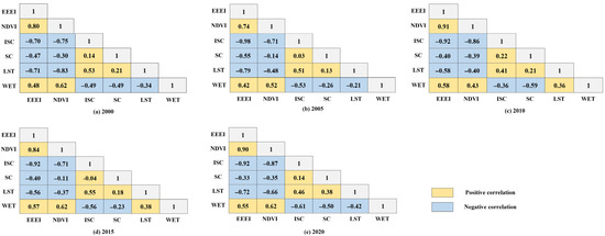
Figure 4.
Correlations among the EEEI and five parameters.
4.2. Ecological Quality Classification and Spatial Distribution of the GBA from 2000 to 2020
The value ranging from 0 to 1 in the EEEI images indicated poor to excellent ecological quality. The images were reclassed to five ecological quality levels on the basis of the mean and standard deviation in this study (Table 5). The results of the ecological quality classification of the GBA from 2000 to 2020 are shown in Figure 5a–e, and the areas and percentage of ecological quality classification are shown in Table 6 and Figure 5f. Generally, the ecological quality of the GBA showed a decreasing trend from 2000 to 2020 (with a mean EEEI of 0.71 for 2000, 0.68 for 2005, 0.69 for 2010, 0.66 for 2015, and 0.64 for 2020), following a first downward, then upward, and finally, a constantly downward trend. Moderate and good ecological qualities were the primary ecological types of the GBA, with a combined percentage of greater than 50% (Figure 5f). Furthermore, the excellent ecological quality changes slightly from 2000 to 2020 with percentages between 10% to 15%, and the areas of excellent types in 2010 are the largest. The areas and percentage of the poor ecological quality showed a constantly increasing trend from 2000 to 2020 (5.47% for 2000, 10.44% for 2005, 12.63% for 2010, 14.31% for 2015, and 17.28% for 2020), primarily due to the expansion of impervious surface areas.
Table 5.
Classification criteria of ecological quality of the GBA from 2000 to 2020.
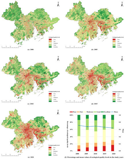
Figure 5.
Ecological quality of the GBA from 2000 to 2020.
Table 6.
Statistics of ecological quality of the GBA from 2000 to 2020.
The spatial distribution of the ecological quality of the GBA generally followed a pattern of “better in edge/coastal area and worse in middle/core area” (Figure 5a–e). The excellent and good types of ecological quality were primarily in Zhaoqing city, Huizhou city, the north of Guangzhou city, and the west of Jiangmen city. Areas with poor and fair types of ecological quality constantly increased and were primarily concentrated in the core areas of the GBA, with clustered distribution in Guangzhou-Dongguan city on the west side of the Pearl River and Shenzhen-Dongguan city on the east side of the Pearl River.
4.3. Change Detection of Ecological Quality of the GBA from 2000 to 2020
To analyze the temporal and spatial changes of ecological quality of the GBA from 2000 to 2020, the detected changes between two adjacent years was analyzed on the basis of EEEI classifications (level 1 to level 5). Therefore, the detected changes in the EEEI were further divided into three levels with nine values ranging from −4 to 4: (1) all positive values indicated that the level of the EEEI improved, classified as “improved”; (2) 0 values indicated that the level of the EEEI remained unchanged, classified as “unchanged”; and (3) all negative values indicated that the level of the EEEI degraded, classified as “degraded”.
The spatial distribution and proportion statistics of ecological quality changes of the GBA in four time periods are shown in Figure 6 and Figure 7. From 2000 to 2005 (Figure 6a and Figure 7a), the degraded values accounted for the highest proportion (47.93%), mainly showing as “degraded with 1 level”. The degraded areas were widely distributed throughout the study area, and the improved areas were mainly located in the north of Guangzhou city and the northwest of Huizhou city. From 2005 to 2010 (Figure 6b and Figure 7b), the unchanged values accounted for the highest proportion (46.35%), followed by the improved and degraded values. Foshan city contained most of the degraded values, whereas other cities were primarily covered by the unchanged and improved values. From 2010 to 2015 (Figure 6c and Figure 7c), the unchanged values accounted for the highest proportion (47.99%), followed by the degraded and improved values. The degraded areas were concentrated in Zhaoqing city and Jiangmen city, with some fragmentary distributions in other cities. The improved areas were mainly located on the edges of Zhaoqing city and Foshan city. From 2015 to 2020 (Figure 6d and Figure 7d), the unchanged values accounted for the highest proportion (45.68%), followed by the degraded and improved values. The degraded areas were mainly located in the southeast of Huizhou city and the edges of Zhaoqing city, Foshan city, and Jiangmen city. The improved areas were mainly concentrated in the north of Huizhou city and the middle and south of Zhaoqing city. It is worth noting that the changes in the improved and degraded were relatively gradual in four time periods, mainly showing as “improved with 1 level” or “degraded with 1 level”.
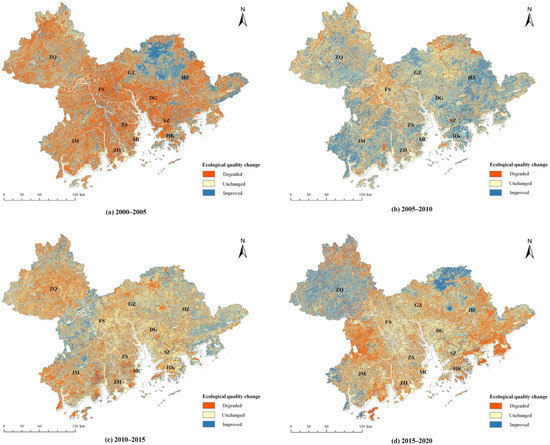
Figure 6.
Spatial distribution ecological quality change of the GBA in four time periods.
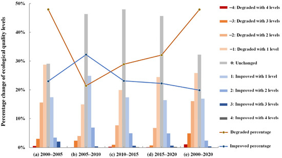
Figure 7.
Percentage changes of ecological quality levels of the GBA from 2000 to 2020.
Furthermore, the detection of changes in ecological quality change of the GBA from 2000 to 2020 was also analyzed in this study. It shows that, overall, the ecological quality of the GBA significantly degraded from 2000 to 2020, and the percentage of the degraded areas reached 47.90% in total (Figure 7e). As shown in Figure 8, the area and percentage with the degraded value accounted for the highest proportions in all cities of the GBA, followed by the unchanged and the improved values.
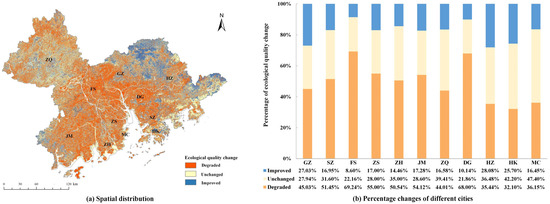
Figure 8.
Ecological quality change of the GBA from 2000 to 2020.
The spatial distribution and the percentage of ecological quality changes in different cities exhibited different trends. In general, the central cities of the GBA exhibited a notable degradation trend and the areas with the improved and unchanged values were mainly in the coastal and edge cities. For ecological quality changes in different cities, there was a rapid degradation in two cities, Foshan, and Dongguan, with 69.24% and 68.00% of the total city area degraded, respectively. The proportion of the improved areas in Huizhou city and Guangzhou city were relatively higher than that in other cities, where 28.08% and 27.03% of the total city area improved, respectively. Additionally, there was relatively gradual changing trends in Hong Kong and Macau, with the proportion of the unchanged values of the total city area accounting for 42.20% and 47.40%, respectively.
5. Discussion
5.1. Significance of the EEEI
With the continuous and rapid increase in human activities and climate change, the eco-environment has been significantly affected and changed at various scales [38,57]. Therefore, how to assess and monitor the spatiotemporal characteristics of ecological status effectively and quickly has become an imperative and challenging research topic. Previous studies have designed a series of ecological indices using various parameters and lacked a comprehensively systematic model to provide an effective ecological evaluation. It is of great importance to develop an efficient and reliable model for ecological assessments. This study developed an enhanced ecological evaluation index (EEEI) which can provide a guidance for scientific, objective, quantitative, and comprehensive ecological quality assessment.
Firstly, the selection of ecological parameters was objective, quantitative, and comprehensive. An appropriate selection of ecological parameters is fundamental for the evaluation of ecological quality. The EEEI was developed based on a clearly designed framework, and the selected five ecological parameters represent land surface ecological quality from greenness, human activities, dryness, heat, and moisture. Notably, the ISC and SC at the sub-pixel level were first used as parameters to evaluate the ecological quality. Specifically, the ISC has a clear physical meaning that can quantify human activities and has been increasingly considered an important and necessary environmental indicator [47,58,59]. Compared with other ecological indices [26,29,38], the assessment results of the EEEI were more intuitive and sensitive to revealing the anthropogenic effects on the ecological status. Therefore, our findings highlight the significance of selecting the ISC as a key parameter to develop the EEEI for ecological quality evaluation.
Secondly, all ecological parameters of the EEEI are easily available, and thus the EEEI can be easily transferable and applicable to other study areas and different datasets. The EEEI needs five ecological parameters as inputs, which can be easily obtained from remote sensing data and methods (Section 2.2). Specifically, all the parameters in this study were quickly calculated and quantified on the basis of Landsat images, and the parameters provide timely and reliable inputs for the EEEI. Additionally, the scale of the EEEI was 30 m × 30 m in this study, which depended on the spatial resolution of the applied remote sensing images. The EEEI is a key application of ecological remote sensing, and it has the potential for assessments of ecological quality to other study areas and different datasets. For example, high spatial resolution images and hyperspectral images (e.g., Sentinel-2, Gaofen-2, Hyperion, MODIS) are available to evaluate ecological quality for local and global regions based on the EEEI. Thus, the proposed EEEI holds a comprehensive ability for ecological quality assessment at various scales.
Furthermore, the assessment results of the EEEI were effective, reasonable, and explicable. As the results revealed, the EEEI could contain most of the information of the five ecological parameters, and the ecological quality evaluation expressed by the EEEI was consistent with the ecological meaning expressed by each of the five parameters (Table 3, Figure 4). Therefore, the EEEI can simultaneously consider the five aspects of land surface ecological conditions (i.e., greenness, human activities, dryness, heat, and moisture), which provided an effective guidance for helping the systematic selection of ecological parameters. Therefore, the EEEI can be used as an effective tool for quantitative and comprehensive ecological quality evaluation.
5.2. Importance for Ecological Protection of the GBA
This study developed the EEEI to assess and detect the ecological quality and spatiotemporal changes of the GBA from 2000 to 2020. Our findings that the ecological quality of the GBA is currently facing great challenges emphasize the significance and urgency for eco-environmental protection of the GBA. Results of ecological quality evaluation based on the EEEI provide important and effective guidance for urban management and ecological protection of the GBA.
As the results revealed, the ecological quality of the GBA showed a degradation trend from 2000 to 2020, and the area and the percentage of poor levels of ecological quality were continuously increased during the past two decades. This is largely due to the expansion of urbanization along with the changes of natural landscapes into anthropogenic impervious surface areas [60,61], inevitably leading to increasing areas with a poor level of ecological quality. Additionally, the moderate and good levels of ecological quality accounted for the highest proportion of the GBA. This indicates that the background quality of the eco-environment contains generally good conditions within the GBA. According to the characteristics of the ecological quality of the GBA, we suggest that decision makers should have a comprehensive and visible understanding on spatial distributions of ecological quality and put in effort to protect and maintain the areas with excellent and good levels of ecological quality, mainly containing forest and grassland. The areas with moderate and fair ecological quality levels need to be monitored for ecological changes to prevent deterioration, and the areas with the poor ecological quality levels urgently need to be repaired and improved, mainly concentrated in core areas with a high degree of urbanization.
It is noteworthy that there was a slightly upward trend in the mean of the EEEI in 2010, showing increasing proportions of the excellent and good levels of ecological quality compared with those of the previous years. Since the reform and opening-up of China in the 1980s, the cities in the bay area underwent rapid urbanization and the eco-environment suffered more destruction. The local government gradually realized the urgency and importance of environmental protection and began to implement environmental policy. For example, the “Grain for Green Project” policy that aims to help restore bare land to grassland or forest was implemented in the Guangdong Province. Additionally, the “Planning of Green Space System” issue was practiced in Shenzhen in 2004, with the goal of protecting and improving the quality of urban green spaces. More importantly, with the theory of the “Scientific Outlook on Development” put forward in 2003, the development of urbanization and industrialization began to focus on environmentally friendly concepts. Thus, driven by protection policies and awareness during this period, the ecological quality exhibited an improvement in 2010. This explains why the mean of the EEEI increased in 2010 to some extent, partially consistent with the results by Chen et al. [40] and Yang et al. [29]. After that, the concept of “Development of GBA” has been gradually put forward since 2015, and the acceleration of urbanization had led to a serious of environmental problems. As the results of the EEEI indicated, the ecological quality experienced a gradual decline after 2015.
From the results of detecting changes in ecological quality, the area and percentage with the degraded values accounted for the highest proportion in all cities of the GBA from 2000 to 2020. It is clear that the degradation of ecological quality was the dominant changing trend in the GBA. With increases in urbanization, regional population, and economic development, natural areas were gradually destroyed by construction in the past 20 years, causing a decrease in ecological quality of the GBA. The spatial distribution and percentage of ecological quality changes in different cities exhibited different trends, partly because of the differences of urbanization levels in different cities. Specifically, Foshan city and Dongguan city exhibited the most notable degradation trend compared with other cities, owing to a fast growth rate of impervious surface in the past 20 years [22]. As two rising cities in the GBA, Foshan city and Dongguan city experienced an accelerated process of urbanization and gradually replaced Guangzhou city and Shenzhen city, respectively, as industrial production bases. Economic development had priority over eco-environment protection, and thus the ecological quality had clear degradation in these two cities. Additionally, the proportion of the unchanged areas of Hong Kong and Macau was higher than that of other cities, accounting for approximately half of the city area from 2000 to 2020. Hong Kong and Macau had been at a mature level of urbanization and focused more on eco-environment conservation, where the ecological quality was well maintained during this period. Therefore, it is necessary to implement corresponding policies of eco-environmental protection according to the urbanization level of different cities. Especially for the rapidly developing cities, the process of urbanization should balance the economic development and ecological protection, avoiding the blindness of urban development. Furthermore, we should observe the spatiotemporal distribution of the ecological quality and focus on the areas with continuous degradation that urgently need to be repaired and improved.
In summary, the EEEI proposed by this study is applicable and provides scientific results of ecological quality evaluation of the GBA that are reasonable and explicable. The spatial distribution of ecological quality levels can be visually quantified and identified, and the changing areas of ecological quality level can be quickly checked and detected for each study period. These findings should provide important information and helpful knowledge for the eco-environmental protection and sustainable development of the GBA.
5.3. Limitations and Future Works
Some limitations and future works need to be discussed. First, the accuracy of the ecological parameters directly affects the performance of the EEEI for ecological quality evaluations. Specifically, it is challenging to obtain accurate results of the ISC and the SC in complex urban surface conditions using medium-resolution images. Applications of multi-source images (i.e., hyperspectral images and high-spatial-resolution images) offer potential to obtain more accurate results of ecological parameters. Second, the ecological quality of water bodies was ignored in this study, and thus the EEEI needs to be improved to add more ecological parameters for the evaluation of water bodies in further research. Third, the temporal coverage of ecological quality evaluation was limited. In this study, we only selected five-time intervals (2000, 2005, 2010, 2015, and 2020) to evaluate ecological quality for the GBA from 2000 to 2020, which could not represent the overall conditions and changing situations of ecological quality during this period. A time-series evaluation of ecological quality should be implemented to better understand the continuous ecological quality and its spatiotemporal changes in further studies.
6. Conclusions
On the basis of remote sensing data and methods, this study developed an enhanced ecological evaluation index (EEEI) with five integrated ecological parameters (NDVI, ISC, SC, LST, and WET), which was proven to be used as an effective ecological index to evaluate ecological quality. The results of the ecological quality evaluated by the EEEI can be visualized in both spatial and temporal ways, and thus the EEEI is suitable for the promotion and application of ecological quality assessments to various areas and scales.
The spatiotemporal characteristics of ecological quality of the GBA from 2000 to 2020 were assessed and detected by using the EEEI. Generally, the ecological quality of the GBA experienced a degradation trend from 2000 to 2020 (with a mean EEEI of 0.71 for 2000, 0.68 for 2005, 0.69 for 2010, 0.66 for 2015, and 0.64 for 2020). The percentage of the poor ecological quality levels increased continuously in the study period, largely owing to the expansion of impervious surface areas. The spatial distribution results indicated that the areas with excellent and good types of ecological quality were mainly distributed in the coastal and edge areas, and the areas with poor level of ecological quality increased constantly and were primarily concentrated in the core cites of the GBA. For temporal and spatial changes, the areas and percentage with the degraded values of ecological quality level accounted for the highest proportion in all cities of the GBA from 2000 to 2020. As the results revealed, the ecological quality of GBA is currently confronted with great challenges. The EEEI can provide effective and intuitive distributions of ecological quality, and can quickly detect the spatiotemporal changes of ecological quality of the GBA. These findings should provide scientific knowledge to help in ecological protection, environmental management, and sustainable development for decision makers of the GBA.
Author Contributions
Conceptualization, resources, supervision, funding acquisition, F.F.; writing original draft, data processing and analysis, investigation, methodology, S.F. All authors have read and agreed to the published version of the manuscript.
Funding
This research was funded by Special Funds for Science and Technology Talent Introduction of Guangdong Academy of Agricultural Sciences (R2022YJ-YB1002), National Natural Science Foundation of China (41901347), Guangdong Basic and Applied Basic Research Foundation (2021A1515011411), Guangdong Basic and Applied Basic Research Foundation (2020A1515010562), Collaborative Innovation Center Project of Guangdong Academy of Agricultural Sciences (XTXM202201), and Rural Sci-tech Special Commissioner Program of Guangzhou (20212100049).
Data Availability Statement
Not applicable.
Conflicts of Interest
The authors declare no conflict of interest.
References
- Borgwardt, F.; Robinson, L.; Trauner, D.; Teixeira, H.; Nogueira, A.J.A.; Lillebo, A.I.; Piet, G.; Kuemmerlen, M.; O’Higgins, T.; McDonald, H.; et al. Exploring variability in environmental impact risk from human activities across aquatic ecosystems. Sci. Total Environ. 2019, 652, 1396–1408. [Google Scholar] [CrossRef] [PubMed]
- Chen, J.; Dong, B.; Li, H.; Zhang, S.; Peng, L.; Fang, L.; Zhang, C.; Li, S. Study on landscape ecological risk assessment of Hooded Crane breeding and overwintering habitat. Environ. Res. 2020, 187, 109649. [Google Scholar] [CrossRef]
- Han, Z.; Song, W.; Deng, X.; Xu, X. Grassland ecosystem responses to climate change and human activities within the Three-River Headwaters region of China. Sci. Rep. 2018, 8, 9079. [Google Scholar] [CrossRef] [Green Version]
- Mahmoud, S.H.; Gan, T.Y. Impact of anthropogenic climate change and human activities on environment and ecosystem services in arid regions. Sci. Total Environ. 2018, 633, 1329–1344. [Google Scholar] [CrossRef] [PubMed]
- McDonnell, M.J.; MacGregor-Fors, I. The ecological future of cities. Science 2016, 352, 936–938. [Google Scholar] [CrossRef] [PubMed]
- Huang, X.; Schneider, A.; Friedl, M.A. Mapping sub-pixel urban expansion in China using MODIS and DMSP/OLS nighttime lights. Remote Sens. Environ. 2016, 175, 92–108. [Google Scholar] [CrossRef]
- Kuang, W.; Liu, J.; Zhang, Z.; Lu, D.; Xiang, B. Spatiotemporal dynamics of impervious surface areas across China during the early 21st century. Chin. Sci. Bull. 2013, 58, 1691–1701. [Google Scholar] [CrossRef] [Green Version]
- Ma, Q.; He, C.; Wu, J.; Liu, Z.; Zhang, Q.; Sun, Z. Quantifying spatiotemporal patterns of urban impervious surfaces in China: An improved assessment using nighttime light data. Landsc. Urban Plan. 2014, 130, 36–49. [Google Scholar] [CrossRef]
- Huang, R.; Nie, Y.; Duo, L.; Zhang, X.; Wu, Z.; Xiong, J. Construction land suitability assessment in rapid urbanizing cities for promoting the implementation of United Nations sustainable development goals: A case study of Nanchang, China. Environ. Sci. Pollut. Res. 2021, 28, 25650–25663. [Google Scholar] [CrossRef]
- Li, Y.; Duo, L.; Zhang, M.; Wu, Z.; Guan, Y. Assessment and estimation of the spatial and temporal evolution of landscape patterns and their impact on habitat quality in Nanchang, China. Land 2021, 10, 1073. [Google Scholar] [CrossRef]
- Alberti, M.; Booth, D.; Hill, K.; Coburn, B.; Avolio, C.; Coe, S.; Spirandelli, D. The impact of urban patterns on aquatic ecosystems: An empirical analysis in Puget lowland sub-basins. Landsc. Urban Plan. 2007, 80, 345–361. [Google Scholar] [CrossRef]
- Wang, Z.; Zhang, S.; Peng, Y.; Wu, C.; Lv, Y.; Xiao, K.; Zhao, J.; Qian, G. Impact of rapid urbanization on the threshold effect in the relationship between impervious surfaces and water quality in shanghai, China. Environ. Pollut. 2020, 267, 115569. [Google Scholar] [CrossRef] [PubMed]
- Xu, H.; Ding, F.; Wen, X. Urban expansion and heat island dynamics in the Quanzhou region, China. IEEE J. Sel. Top. Appl. Earth Observ. Remote Sens. 2009, 2, 74–79. [Google Scholar] [CrossRef]
- Yuan, F.; Bauer, M.E. Comparison of impervious surface area and normalized difference vegetation index as indicators of surface urban heat island effects in Landsat imagery. Remote Sens. Environ. 2007, 106, 375–386. [Google Scholar] [CrossRef]
- Zhao, Z.; Sharifi, A.; Dong, X.; Shen, L.; He, B. Spatial variability and temporal heterogeneity of surface urban heat island patterns and the suitability of local climate zones for land surface temperature characterization. Remote Sens. 2021, 13, 4338. [Google Scholar] [CrossRef]
- Dams, J.; Dujardin, J.; Reggers, R.; Bashir, I.; Canters, F.; Batelaan, O. Mapping impervious surface change from remote sensing for hydrological modeling. J. Hydrol. 2013, 485, 84–95. [Google Scholar] [CrossRef]
- Jacobson, C.R. Identification and quantification of the hydrological impacts of imperviousness in urban catchments: A review. J. Environ. Manag. 2011, 92, 1438–1448. [Google Scholar] [CrossRef]
- Daskalova, G.N.; Myers-Smith, I.H.; Bjorkman, A.D.; Blowes, S.A.; Supp, S.R.; Magurran, A.E.; Dornelas, M. Landscape-scale forest loss as a catalyst of population and biodiversity change. Science 2020, 368, 1341. [Google Scholar] [CrossRef]
- Gillies, R.R.; Box, J.B.; Symanzik, J.; Rodemaker, E.J. Effects of urbanization on the aquatic fauna of the Line Creek watershed, Atlanta—A satellite perspective. Remote Sens. Environ. 2003, 86, 411–422. [Google Scholar] [CrossRef] [Green Version]
- Coutts, A.M.; Harris, R.J.; Phan, T.; Livesley, S.J.; Williams, N.S.G.; Tapper, N.J. Thermal infrared remote sensing of urban heat: Hotspots, vegetation, and an assessment of techniques for use in urban planning. Remote Sens. Environ. 2016, 186, 637–651. [Google Scholar] [CrossRef]
- Estoque, R.C.; Murayama, Y. Monitoring surface urban heat island formation in a tropical mountain city using Landsat data (1987–2015). ISPRS J. Photogramm. Remote Sens. 2017, 133, 18–29. [Google Scholar] [CrossRef]
- Feng, S.; Fan, F. Spatiotemporal changes of landscape pattern using impervious surface in Guangdong-Hong Kong-Macao Greater Bay Area, China. Chin. J. Appli. Ecol. 2018, 29, 2907–2914. (In Chinese) [Google Scholar]
- Gupta, K.; Kumar, P.; Pathan, S.K.; Sharma, K.P. Urban neighborhood green index—A measure of green spaces in urban areas. Landsc. Urban Plan. 2012, 105, 325–335. [Google Scholar] [CrossRef]
- Hua, L.; Zhang, X.; Nie, Q.; Sun, F.; Tang, L. The impacts of the expansion of urban impervious surfaces on urban heat islands in a coastal city in China. Sustainability 2020, 12, 475. [Google Scholar] [CrossRef] [Green Version]
- Sullivan, C.A.; Skeffington, M.S.; Gormally, M.J.; Finn, J.A. The ecological status of grasslands on lowland farmlands in western Ireland and implications for grassland classification and nature value assessment. Biol. Conserv. 2010, 143, 1529–1539. [Google Scholar] [CrossRef]
- Xu, H. A remote sensing urban ecological index and its application. Acta Ecol. Sin. 2013, 33, 7853–7862. (In Chinese) [Google Scholar]
- Liao, W.; Jiang, W. Evaluation of the spatiotemporal variations in the eco-environmental quality in China based on the remote sensing ecological index. Remote Sens. 2020, 12, 2462. [Google Scholar] [CrossRef]
- Xu, H.; Wang, Y.; Guan, H.; Shi, T.; Hu, X. Detecting ecological changes with a remote sensing based ecological index (RSEI) Produced Time Series and Change Vector Analysis. Remote Sens. 2019, 11, 2345. [Google Scholar] [CrossRef] [Green Version]
- Yang, C.; Zhang, C.; Li, Q.; Liu, H.; Gao, W.; Shi, T.; Liu, X.; Wu, G. Rapid urbanization and policy variation greatly drive ecological quality evolution in Guangdong-Hong Kong-Macau Greater Bay Area of China: A remote sensing perspective. Ecol. Indic. 2020, 115, 106373. [Google Scholar] [CrossRef]
- Hu, X.; Hong, W.; Qiu, R.; Hong, T.; Chen, C.; Wu, C. Geographic variations of ecosystem service intensity in Fuzhou City, China. Sci. Total Environ. 2015, 512–513, 215–226. [Google Scholar] [CrossRef]
- Hu, X.; Xu, H. A new remote sensing index for assessing the spatial heterogeneity in urban ecological quality: A case from Fuzhou City, China. Ecol. Indic. 2018, 89, 11–21. [Google Scholar] [CrossRef]
- Yue, H.; Liu, Y.; Li, Y.; Lu, Y. Eco-environmental quality assessment in China’s 35 major cities based on remote sensing ecological index. IEEE Access 2019, 7, 51295–51311. [Google Scholar] [CrossRef]
- Zhu, D.; Chen, T.; Zhen, N.; Niu, R. Monitoring the effects of open-pit mining on the eco-environment using a moving window-based remote sensing ecological index. Environ. Sci. Pollut. Res. 2020, 27, 15716–15728. [Google Scholar] [CrossRef] [PubMed]
- Guo, B.; Fang, Y.; Jin, X.; Zhou, Y. Monitoring the effects of land consolidation on the ecological environmental quality based on remote sensing: A case study of Chaohu Lake Basin, China. Land Use Policy 2020, 95, 104569. [Google Scholar] [CrossRef]
- Jing, Y.; Zhang, F.; He, Y.; Kung, H.; Johnson, V.C.; Arikena, M. Assessment of spatial and temporal variation of ecological environment quality in Ebinur Lake Wetland National Nature Reserve, Xinjiang, China. Ecol. Indic. 2020, 110, 105874. [Google Scholar] [CrossRef]
- Wang, J.; Ma, J.; Xie, F.; Xu, X. Improvement of remote sensing ecological index in arid regions: Taking Ulan Buh Desert as an example. Chin. J. Appl. Ecol. 2020, 31, 3795–3804. (In Chinese) [Google Scholar]
- Song, M.; Luo, Y.; Duan, L. Evaluation of ecological environment in the Xilin Gol Steppe based on modified remote sensing ecological index model. Arid. Zone Res. 2019, 36, 1521–1527. (In Chinese) [Google Scholar]
- He, C.; Gao, B.; Huang, Q.; Ma, Q.; Dou, Y. Environmental degradation in the urban areas of China: Evidence from multi-source remote sensing data. Remote Sens. Environ. 2017, 193, 65–75. [Google Scholar] [CrossRef]
- Firozjaei, M.K.; Fathololoumi, S.; Weng, Q.; Kiavarz, M.; Alavipanah, S.K. Remotely Sensed Urban Surface Ecological Index (RSUSEI): An Analytical Framework for Assessing the Surface Ecological Status in Urban Environments. Remote Sens. 2020, 12, 2029. [Google Scholar] [CrossRef]
- Chen, X.; Li, F.; Li, X.; Hu, Y.; Wang, Y. Mapping ecological space quality changes for ecological management: A case study in the Pearl River Delta urban agglomeration, China. J. Environ. Manag. 2020, 267, 110658. [Google Scholar] [CrossRef]
- Ding, Q.; Wang, L.; Fu, M.; Huang, N. An integrated system for rapid assessment of ecological quality based on remote sensing data. Environ. Sci. Pollut. Res. 2020, 27, 32779–32795. [Google Scholar] [CrossRef] [PubMed]
- Seddon, A.W.R.; Macias-Fauria, M.; Long, P.R.; Benz, D.; Willis, K.J. Sensitivity of global terrestrial ecosystems to climate variability. Nature 2016, 531, 229–232. [Google Scholar] [CrossRef] [PubMed] [Green Version]
- Crist, E.P. A TM tasseled cap equivalent transformation for reflectance factor data. Remote Sens. Environ. 1985, 17, 301–306. [Google Scholar] [CrossRef]
- Zhao, H.; Chen, X. Use of normalized difference bareness index in quickly mapping bare areas from TM/ETM+. In Proceedings of the IEEE International Geoscience and Remote Sensing Symposium (IGARSS), Seoul, Korea, 29 July 2005; pp. 1666–1668. [Google Scholar]
- Lu, D.; Li, G.; Kuang, W.; Moran, E. Methods to extract impervious surface areas from satellite images. Int. J. Digit. Earth 2014, 7, 93–112. [Google Scholar] [CrossRef]
- Weng, Q. Remote sensing of impervious surfaces in the urban areas: Requirements, methods, and trends. Remote Sens. Environ. 2012, 117, 34–49. [Google Scholar] [CrossRef]
- Wu, W.; Li, C.; Liu, M.; Hu, Y.; Xiu, C. Change of impervious surface area and its impacts on urban landscape: An example of Shenyang between 2010 and 2017. Ecosyst. Health Sustain. 2020, 6, 1767511. [Google Scholar] [CrossRef]
- Hughey, K.F.D.; Cullen, R.; Kerr, G.N.; Cook, A.J. Application of the pressure-state-response framework to perceptions reporting of the state of the New Zealand environment. J. Environ. Manag. 2004, 70, 85–93. [Google Scholar] [CrossRef] [Green Version]
- Niemi, G.J.; McDonald, M.E. Application of ecological indicators. Annu. Rev. Ecol. Evol. Syst. 2004, 35, 89–111. [Google Scholar] [CrossRef] [Green Version]
- Wu, C.; Murray, A.T. Estimating impervious surface distribution by spectral mixture analysis. Remote Sens. Environ. 2003, 84, 493–505. [Google Scholar] [CrossRef]
- Adams, J. Classification of multispectral images based on fractions of endmembers: Application to land-cover change in the Brazilian Amazon. Remote Sens. Environ. 1995, 52, 137–154. [Google Scholar] [CrossRef]
- Roberts, D.A.; Gardner, M.; Church, R.; Ustin, S.; Scheer, G.; Green, R.O. Mapping chaparral in the Santa Monica Mountains using multiple endmember spectral mixture models. Remote Sens. Environ. 1998, 65, 267–279. [Google Scholar] [CrossRef]
- Zha, Y.; Gao, J.; Ni, S. Use of normalized difference built-up index in automatically mapping urban areas from TM imagery. Int. J. Remote Sens. 2003, 24, 583–594. [Google Scholar] [CrossRef]
- Chander, G.; Markham, B.L.; Helder, D.L. Summary of current radiometric calibration coefficients for Landsat MSS, TM, ETM+, and EO-1 ALI sensors. Remote Sens. Environ. 2009, 113, 893–903. [Google Scholar] [CrossRef]
- Nichol, J. Remote sensing of urban heat islands by day and night. Photogramm. Eng. Remote Sens. 2005, 71, 613–621. [Google Scholar] [CrossRef]
- Xu, H. Modification of normalised difference water index (NDWI) to enhance open water features in remotely sensed imagery. Int. J. Remote Sens. 2006, 27, 3025–3033. [Google Scholar] [CrossRef]
- Yu, Z.; Yao, Y.; Yang, G.; Wang, X.; Vejre, H. Strong contribution of rapid urbanization and urban agglomeration development to regional thermal environment dynamics and evolution. For. Ecol. Manag. 2019, 446, 214–225. [Google Scholar] [CrossRef]
- Powell, S.; Cohen, W.; Yang, Z.; Pierce, J.; Alberti, M. Quantification of impervious surface in the Snohomish Water Resources Inventory Area of Western Washington from 1972–2006. Remote Sens. Environ. 2007, 112, 1895–1908. [Google Scholar] [CrossRef] [Green Version]
- Ramamurthy, P.; Bou-Zeid, E. Contribution of impervious surfaces to urban evaporation. Water Resour. Res. 2014, 50, 2889–2902. [Google Scholar] [CrossRef]
- Xu, R.; Zhang, H.; Lin, H. Annual dynamics of impervious surfaces at city level of Pearl River Delta metropolitan. Int. J. Remote Sens. 2018, 39, 3537–3555. [Google Scholar] [CrossRef]
- Zhang, L.; Weng, Q. Annual dynamics of impervious surface in the Pearl River Delta, China, from 1988 to 2013, using time series Landsat imagery. ISPRS J. Photogramm. Remote Sens. 2016, 113, 86–96. [Google Scholar] [CrossRef]
Publisher’s Note: MDPI stays neutral with regard to jurisdictional claims in published maps and institutional affiliations. |
© 2022 by the authors. Licensee MDPI, Basel, Switzerland. This article is an open access article distributed under the terms and conditions of the Creative Commons Attribution (CC BY) license (https://creativecommons.org/licenses/by/4.0/).