
A Framework for Multivariate Analysis of Land Surface Dynamics and Driving Variables—A Case Study for Indo-Gangetic River Basins


Abstract
:
1. Introduction
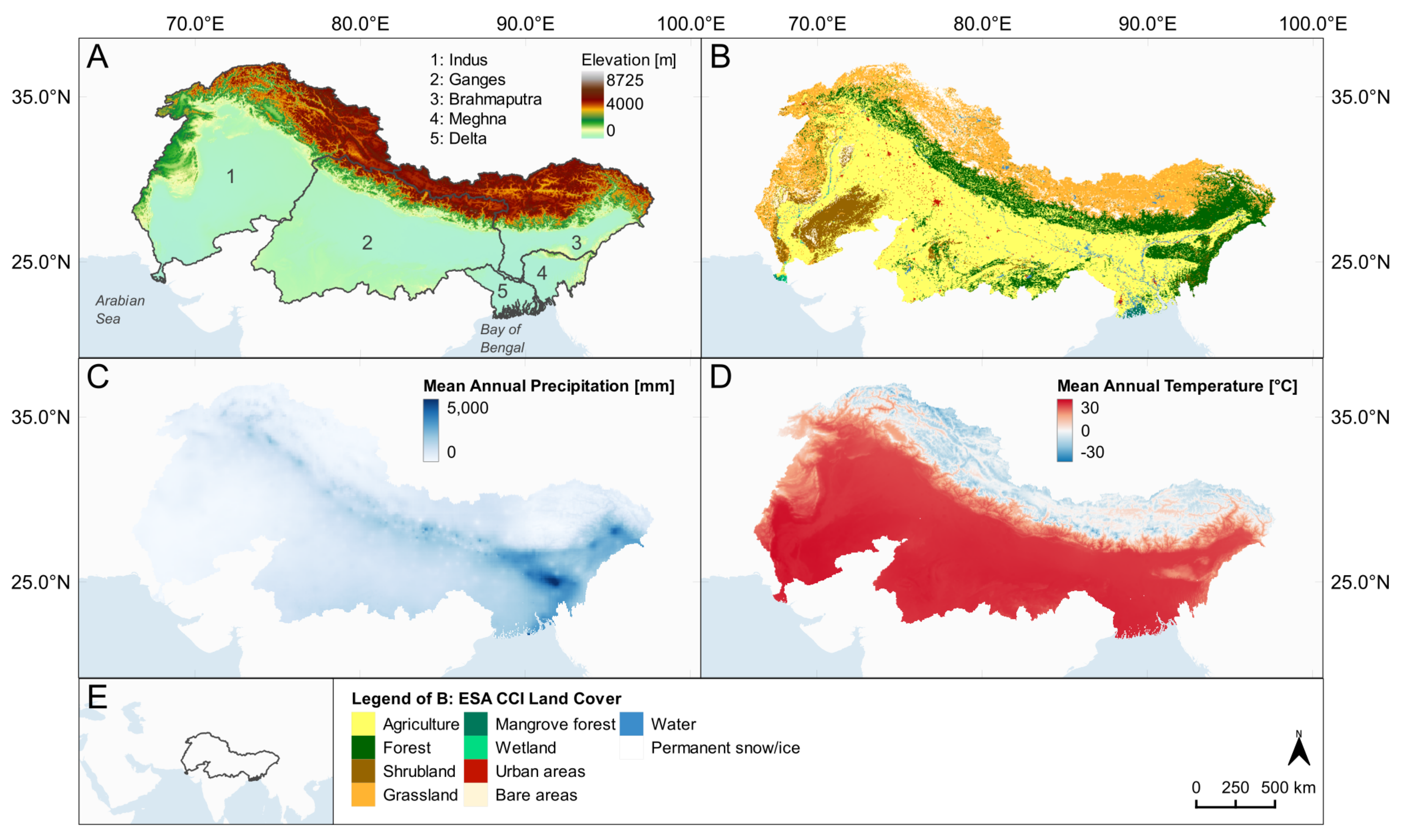
2. Study Area
3. Materials and Methods
3.1. Data
3.1.1. MODIS NDVI
3.1.2. Global Snowpack (GSP)
3.1.3. Global Waterpack (GWP)
3.1.4. Climatological and Hydrological Data
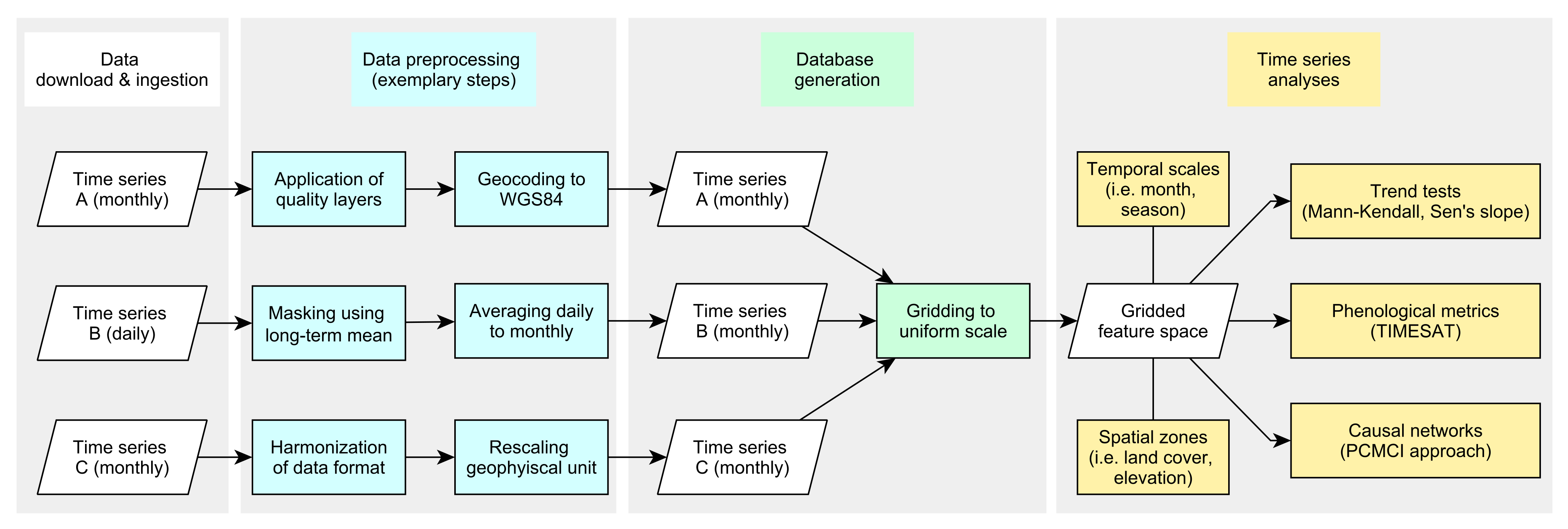
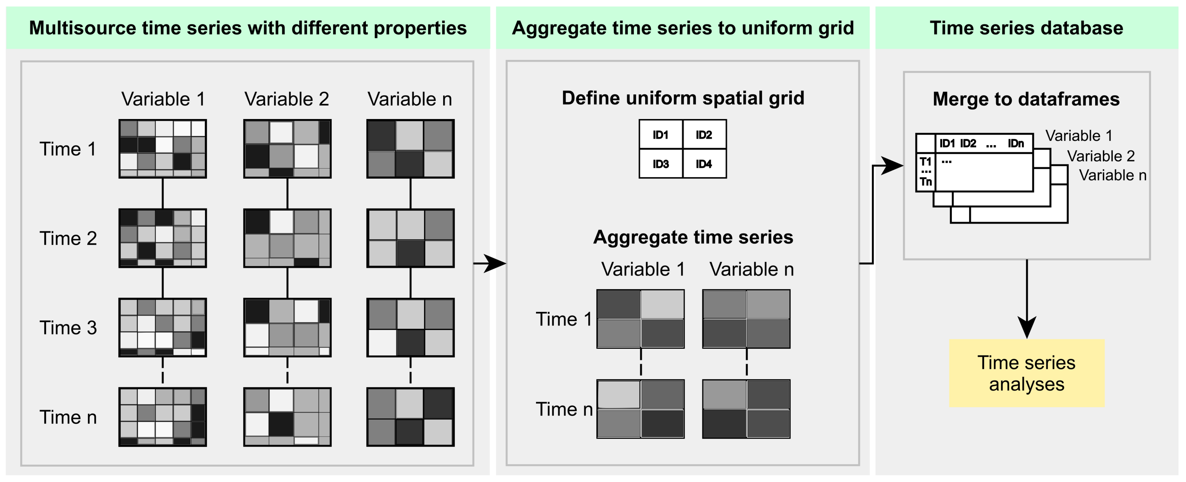
3.2. Database Generation
3.3. Time Series Analyses
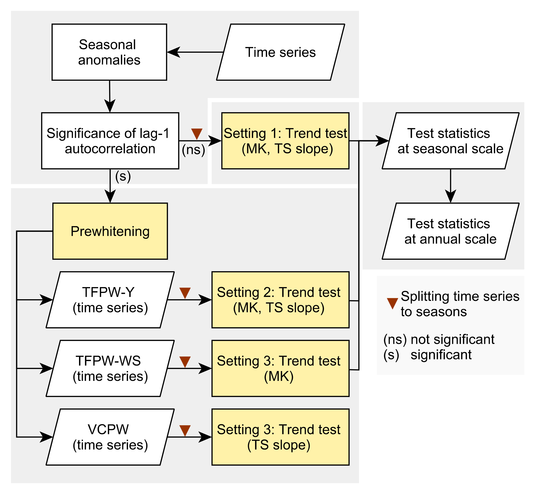
3.3.1. Trend Tests
3.3.2. Seasonality Analysis
3.3.3. Causal Discovery Algorithm
4. Results
4.1. Trends
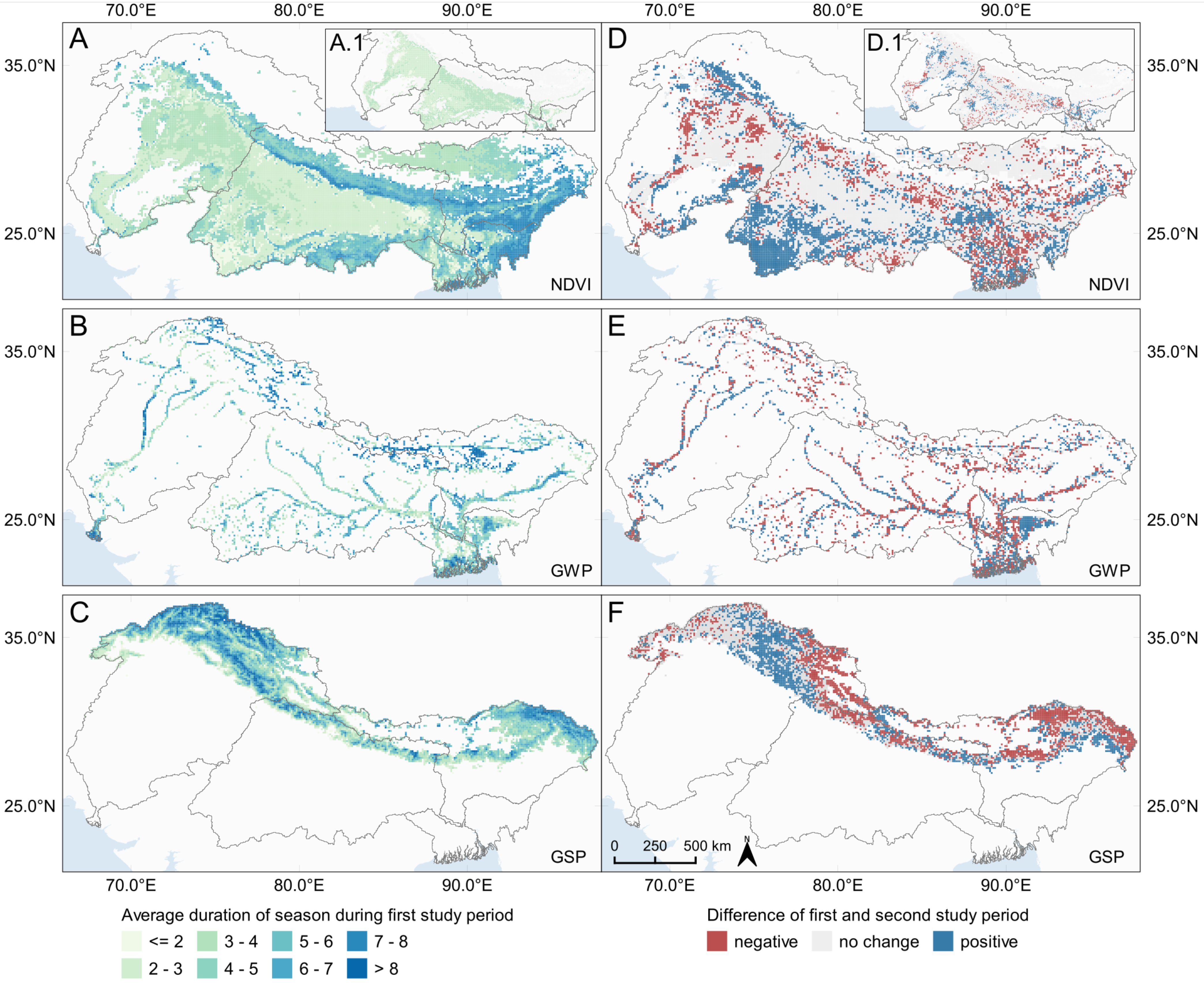
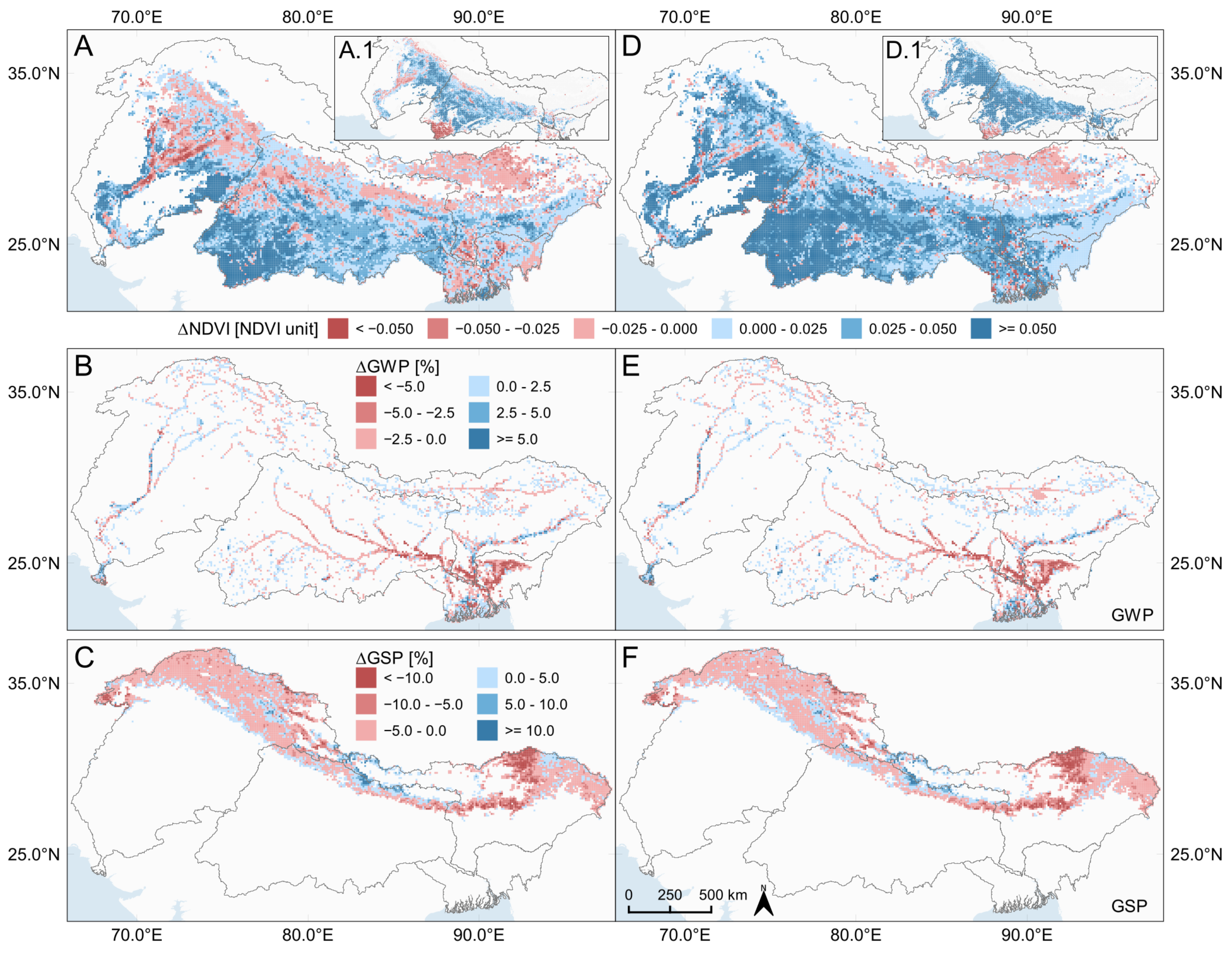
4.2. Seasonal Characteristics
4.3. Relation with Climatic and Hydrological Drivers
5. Discussion
5.1. Trends and Seasonality
5.2. Analysis of Causal Links
5.3. Limitations and Future Requirements
6. Conclusions
- Seasonality and autocorrelation must be dealt with when using the Mann–Kendall test. Thus, we used the seasonal Mann–Kendall test on pre-whitened time series keeping the monthly resolution. At the same time, advantages and disadvantages of pre-whitening algorithms need to be considered. In this regard, experiments suggest not to rely on only a single algorithm;
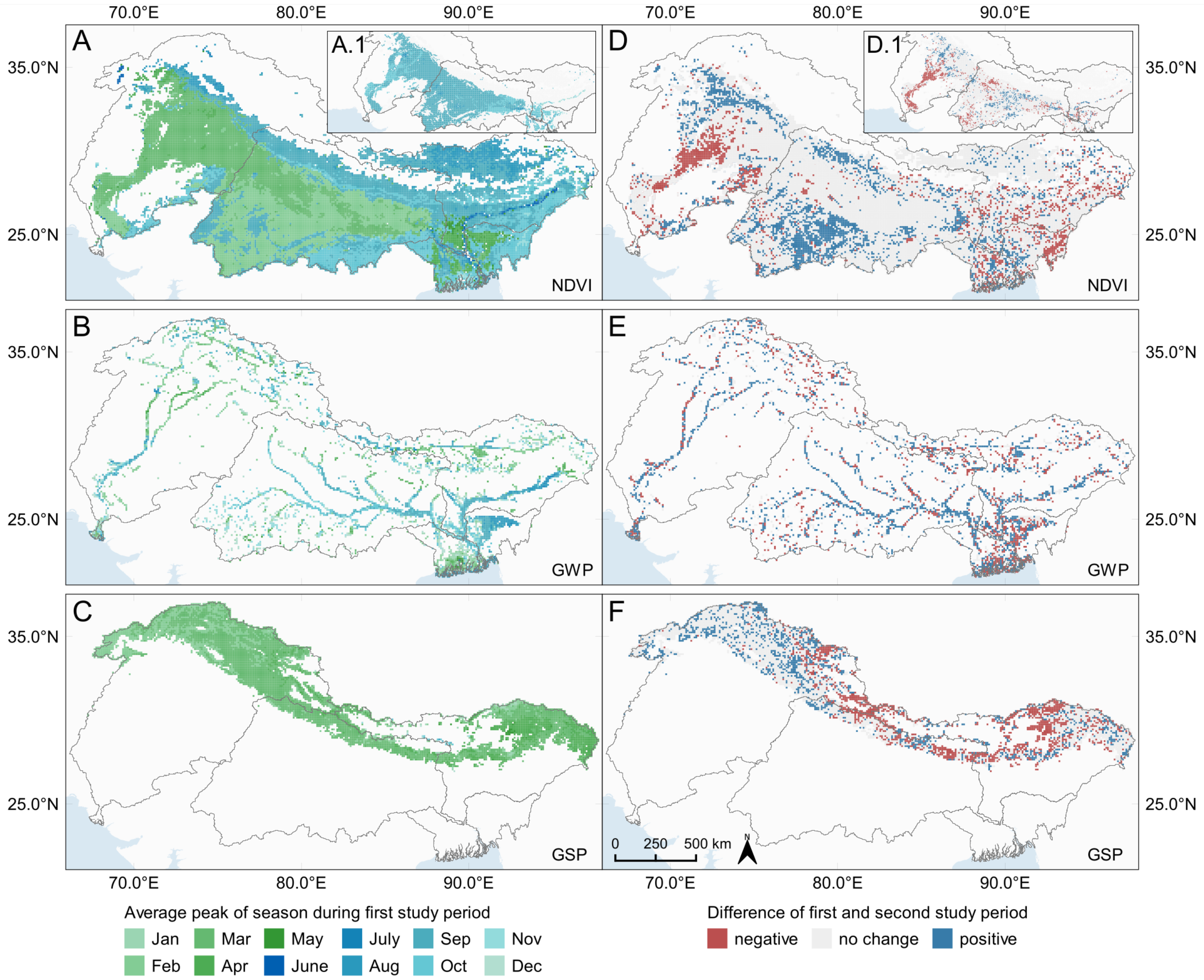
- Through application of Timesat, we examined the existence of seasonal changes between two decades. For NDVI, we used a global setting considering areas with one and two growing seasons. Although we used monthly time series, we found that the retrieved phenological metrics show consistency with the spatial patterns of positive and negative trends;
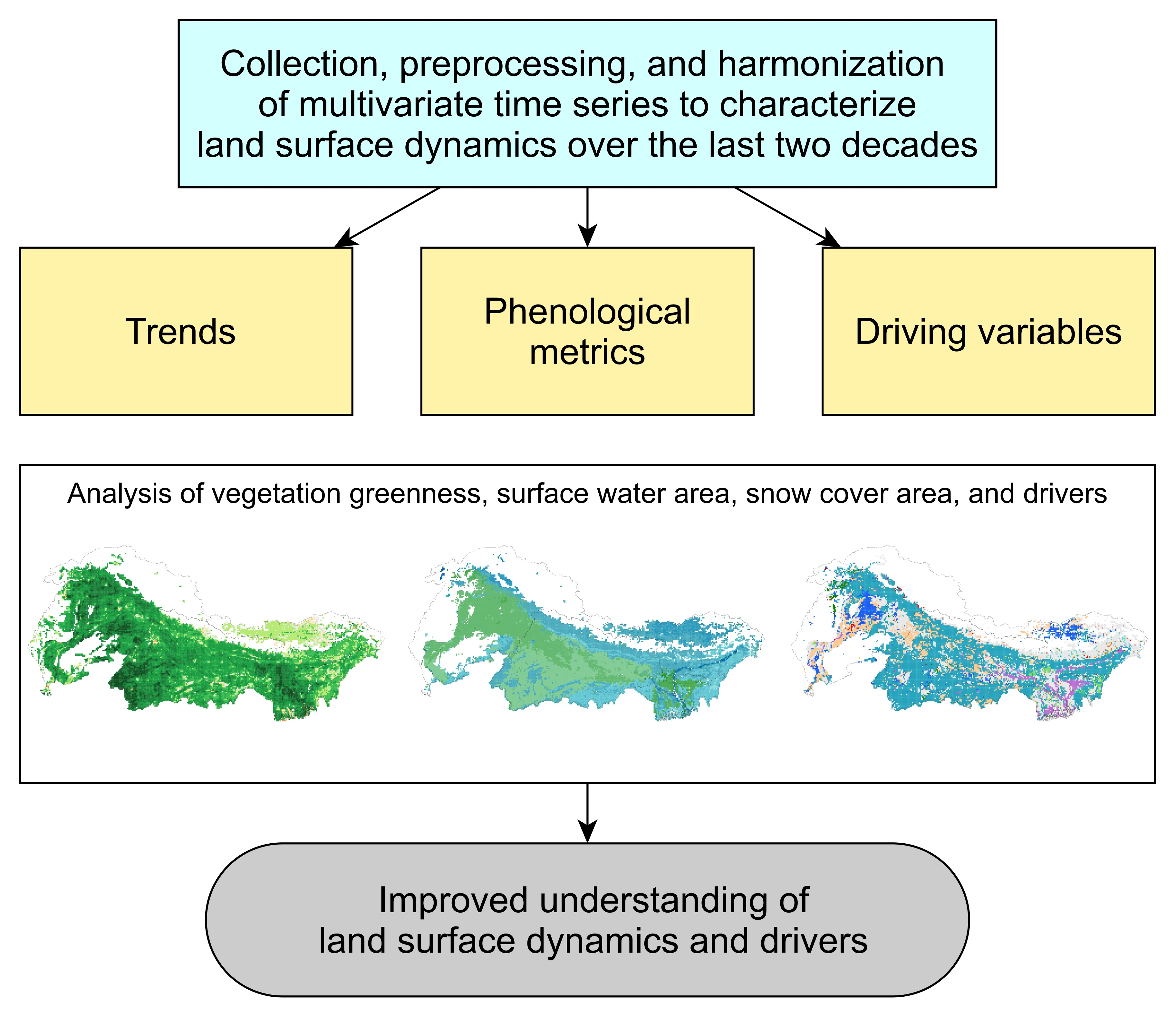
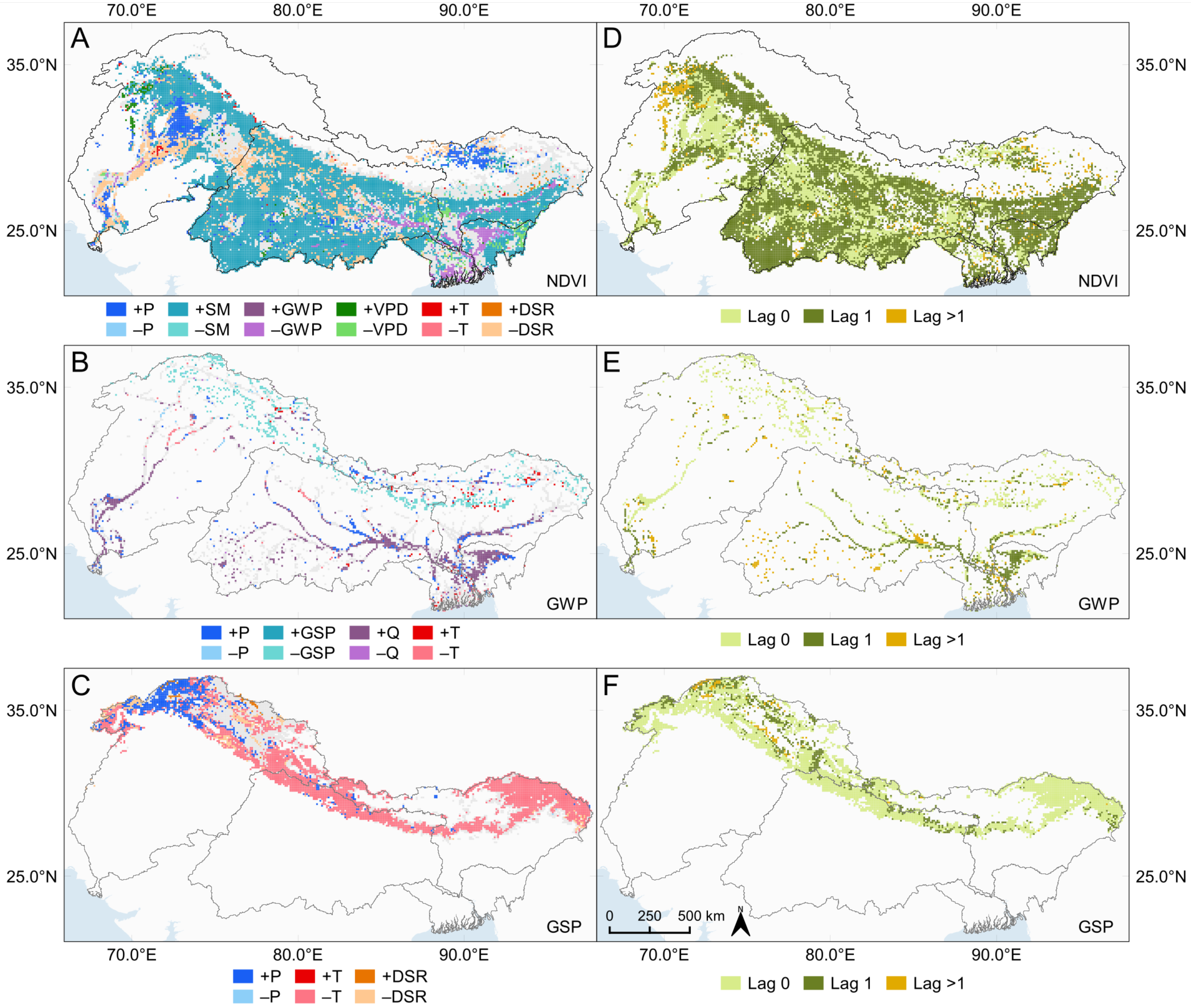
- This study is the first to use such a high dimensional feature space for the quantification of drivers of vegetation greenness, surface water area, and snow cover area using the causal discovery algorithm PCMCI. The dependencies between the target and driving variables indicate consistent and homogeneous patterns, confirming its functionality.
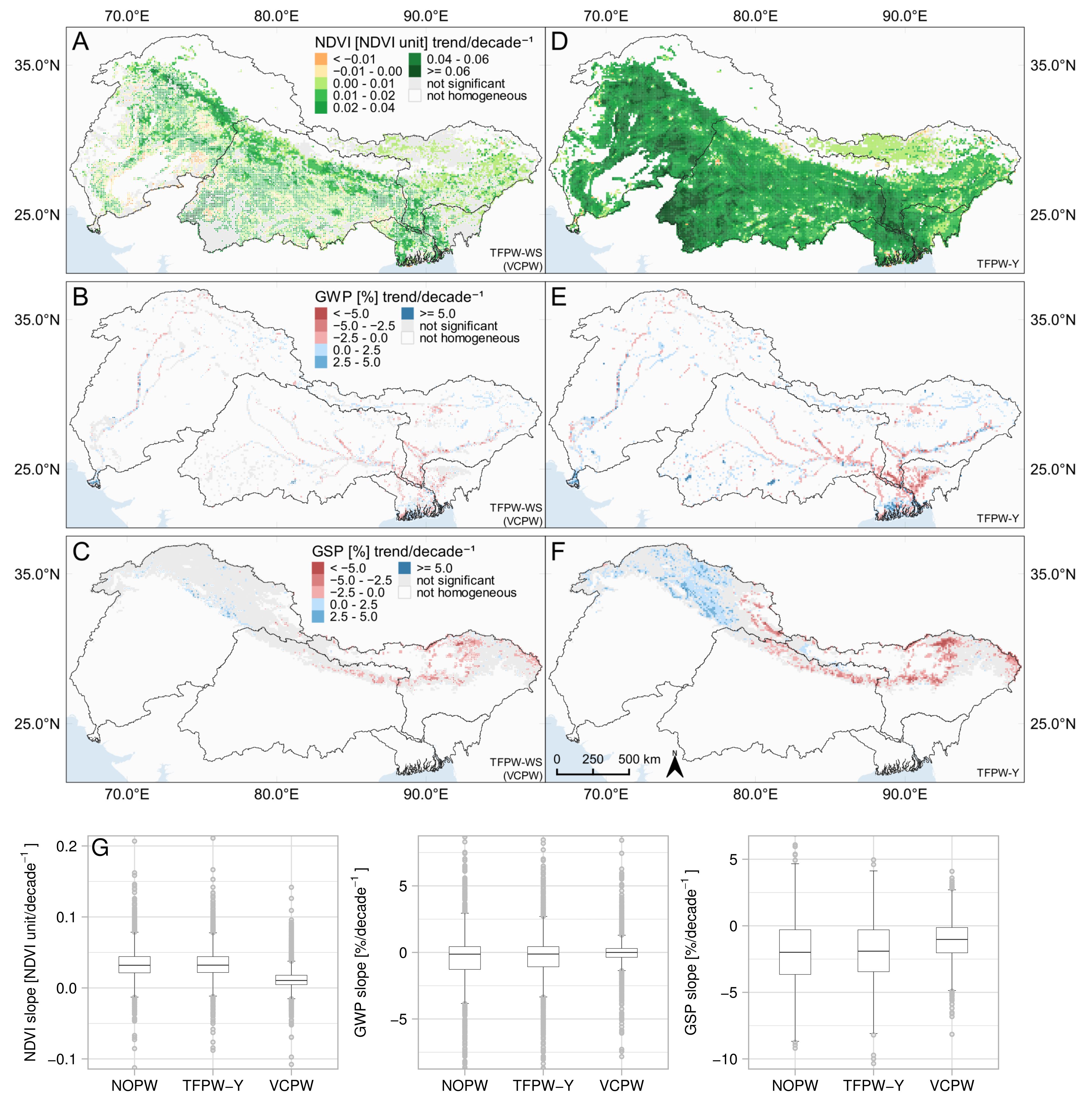
- MODIS NDVI indicates that greening trends are dominant downstream of the Himalaya-Karakoram. Seasonality of NDVI indicates decreasing seasonal amplitude being accompanied by stable or increasing seasonal peak values. Hence, greening of vegetation in this region is ongoing. We also found that NDVI is mostly impacted by water availability;
- According to the DLR Global Waterpack, negative trends are prominent at the confluence of the Ganges and Brahmaputra rivers and in wetlands of the Meghna basin. Positive trends occur north of the Bay of Bengal and in the Southwest of the Ganges basin. In high altitudes, snow cover and temperature influence surface water area. In the lower river basins, we found discharge and precipitation to be of high relevance;
- The DLR Global Snowpack indicates weak increasing trends over the Upper Indus river basin. Negative trends prevail in the Upper Ganges and Brahmaputra river basins. Accordingly, our results demonstrate that changes in duration of snow cover area match spatial patterns of detected significant trends. Snow cover is largely negatively coupled to temperature, while precipitation shows positive influence over the western Upper Indus river basin.
Supplementary Materials
Author Contributions
Funding
Institutional Review Board Statement
Informed Consent Statement
Data Availability Statement
Acknowledgments
Conflicts of Interest
References
- Jia, G.; Shevliakova, E.; Artaxo, P.; Noblet-Ducoudré, D.; Houghton, R.; House, J.; Kitajima, K.; Lennard, C.; Popp, A.; Sirin, A. Land-climate interactions. In Climate Change and Land: An IPCC Special Report on Climate Change, Desertification, Land Degradation, Sustainable Land Management, Food Security, and Greenhouse Gas Fluxes in Terrestrial Ecosystems; Shukla, P.R., Skea, J., Calvo Buendi, E., Masson-Delmotte, V., Pörtner, H.O., Roberts, D.C., Zhai, P., Slade, R., Connors, S., Diemen, R.V., et al., Eds.; Cambridge University Press: Cambridge, UK, 2019; pp. 131–247. [Google Scholar]
- Piao, S.; Wang, X.; Park, T.; Chen, C.; Lian, X.; He, Y.; Bjerke, J.W.; Chen, A.; Ciais, P.; Tømmervik, H.; et al. Characteristics, drivers and feedbacks of global greening. Nat. Rev. Earth Environ. 2020, 1, 14–27. [Google Scholar] [CrossRef]
- de Beurs, K.M.; Henebry, G.M. A statistical framework for the analysis of long image time series. Int. J. Remote Sens. 2005, 26, 1551–1573. [Google Scholar] [CrossRef]
- Kuenzer, C.; Dech, S.; Wagner, W. Remote Sensing Time Series Revealing Land Surface Dynamics: Status Quo and the Pathway Ahead. In Remote Sensing Time Series; Remote Sensing and Digital Image Processing; Springer: Cham, Switzerland, 2015; Book Section Chapter 1; pp. 1–24. [Google Scholar] [CrossRef]
- Reichstein, M.; Camps-Valls, G.; Stevens, B.; Jung, M.; Denzler, J.; Carvalhais, N.; Prabhat. Deep learning and process understanding for data-driven Earth system science. Nature 2019, 566, 195–204. [Google Scholar] [CrossRef] [PubMed]
- Duan, S.B.; Li, Z.L.; Li, H.; Göttsche, F.M.; Wu, H.; Zhao, W.; Leng, P.; Zhang, X.; Coll, C. Validation of Collection 6 MODIS land surface temperature product using in situ measurements. Remote Sens. Environ. 2019, 225, 16–29. [Google Scholar] [CrossRef] [Green Version]
- Zhao, M.; Heinsch, F.A.; Nemani, R.R.; Running, S.W. Improvements of the MODIS terrestrial gross and net primary production global data set. Remote Sens. Environ. 2005, 95, 164–176. [Google Scholar] [CrossRef]
- Wang, D.; Liang, S.; He, T.; Yu, Y.; Schaaf, C.; Wang, Z. Estimating daily mean land surface albedo from MODIS data. J. Geophys. Res. Atmos. 2015, 120, 4825–4841. [Google Scholar] [CrossRef]
- Didan, K.; Munoz, A.B.; Solano, R.; Huete, A. MODIS Vegetation Index User’s Guide (MOD13 Series); Vegetation Index and Phenology Lab, University of Arizona: Tucson, AZ, USA, 2015. [Google Scholar]
- Claverie, M.; Matthews, J.; Vermote, E.; Justice, C. A 30+ Year AVHRR LAI and FAPAR Climate Data Record: Algorithm Description and Validation. Remote Sens. 2016, 8, 263. [Google Scholar] [CrossRef] [Green Version]
- Hansen, M.C.; Potapov, P.V.; Moore, R.; Hancher, M.; Turubanova, S.A.; Tyukavina, A.; Thau, D.; Stehman, S.V.; Goetz, S.J.; Loveland, T.R.; et al. High-Resolution Global Maps of 21st-Century Forest Cover Change. Science 2013, 342, 850–853. [Google Scholar] [CrossRef] [PubMed] [Green Version]
- Pekel, J.F.; Cottam, A.; Gorelick, N.; Belward, A.S. High-resolution mapping of global surface water and its long-term changes. Nature 2016, 540, 418. [Google Scholar] [CrossRef]
- Klein, I.; Gessner, U.; Dietz, A.J.; Kuenzer, C. Global WaterPack—A 250 m resolution dataset revealing the daily dynamics of global inland water bodies. Remote Sens. Environ. 2017, 198, 345–362. [Google Scholar] [CrossRef]
- Dietz, A.J.; Kuenzer, C.; Dech, S. Global SnowPack: A new set of snow cover parameters for studying status and dynamics of the planetary snow cover extent. Remote Sens. Lett. 2015, 6, 844–853. [Google Scholar] [CrossRef]
- Naegeli, K.; Neuhaus, C.; Salberg, A.B.; Schwaizer, G.; Wiesmann, A.; Wunderle, S.; Nagler, T. ESA Snow Climate Change initiative (Snow_cci): Daily Global Snow Cover Fraction—Snow on Ground (SCFG) from AVHRR (1982–2019), Version 1.0. NERC EDS Centre for Environmental Data Analysis. Available online: https://catalogue.ceda.ac.uk/uuid/5484dc1392bc43c1ace73ba38a22ac56 (accessed on 1 September 2021).
- Marconcini, M.; Metz-Marconcini, A.; Ureyen, S.; Palacios-Lopez, D.; Hanke, W.; Bachofer, F.; Zeidler, J.; Esch, T.; Gorelick, N.; Kakarla, A.; et al. Outlining where humans live, the World Settlement Footprint 2015. Sci. Data 2020, 7, 242. [Google Scholar] [CrossRef]
- Pesaresi, M.; Huadong, G.; Blaes, X.; Ehrlich, D.; Ferri, S.; Gueguen, L.; Halkia, M.; Kauffmann, M.; Kemper, T.; Lu, L. A global human settlement layer from optical HR/VHR RS data: Concept and first results. IEEE J. Sel. Top. Appl. Earth. Obs. Remote Sens. 2013, 6, 2102–2131. [Google Scholar] [CrossRef]
- Mahecha, M.D.; Gans, F.; Brandt, G.; Christiansen, R.; Cornell, S.E.; Fomferra, N.; Kraemer, G.; Peters, J.; Bodesheim, P.; Camps-Valls, G.; et al. Earth system data cubes unravel global multivariate dynamics. Earth Syst. Dynam. 2020, 11, 201–234. [Google Scholar] [CrossRef] [Green Version]
- Salcedo-Sanz, S.; Ghamisi, P.; Piles, M.; Werner, M.; Cuadra, L.; Moreno-Martínez, A.; Izquierdo-Verdiguier, E.; Muñoz-Marí, J.; Mosavi, A.; Camps-Valls, G. Machine learning information fusion in Earth observation: A comprehensive review of methods, applications and data sources. Inf. Fusion 2020, 63, 256–272. [Google Scholar] [CrossRef]
- Steffen, W.; Richardson, K.; Rockström, J.; Schellnhuber, H.J.; Dube, O.P.; Dutreuil, S.; Lenton, T.M.; Lubchenco, J. The emergence and evolution of Earth System Science. Nat. Rev. Earth Environ. 2020, 1, 54–63. [Google Scholar] [CrossRef] [Green Version]
- Sudmanns, M.; Tiede, D.; Lang, S.; Bergstedt, H.; Trost, G.; Augustin, H.; Baraldi, A.; Blaschke, T. Big Earth data: Disruptive changes in Earth observation data management and analysis? Int. J. Digit. Earth 2019, 13, 832–850. [Google Scholar] [CrossRef]
- Gorelick, N.; Hancher, M.; Dixon, M.; Ilyushchenko, S.; Thau, D.; Moore, R. Google Earth Engine: Planetary-scale geospatial analysis for everyone. Remote Sens. Environ. 2017, 202, 18–27. [Google Scholar] [CrossRef]
- Baumann, P.; Rossi, A.P.; Bell, B.; Clements, O.; Evans, B.; Hoenig, H.; Hogan, P.; Kakaletris, G.; Koltsida, P.; Mantovani, S.; et al. Fostering Cross-Disciplinary Earth Science Through Datacube Analytics. In Earth Observation Open Science and Innovation; Springer: Cham, Switzerland, 2018; Book Section Chapter 5; pp. 91–119. [Google Scholar] [CrossRef] [Green Version]
- Simoes, R.; Camara, G.; Queiroz, G.; Souza, F.; Andrade, P.R.; Santos, L.; Carvalho, A.; Ferreira, K. Satellite Image Time Series Analysis for Big Earth Observation Data. Remote Sens. 2021, 13, 2428. [Google Scholar] [CrossRef]
- Lewis, A.; Oliver, S.; Lymburner, L.; Evans, B.; Wyborn, L.; Mueller, N.; Raevksi, G.; Hooke, J.; Woodcock, R.; Sixsmith, J.; et al. The Australian Geoscience Data Cube—Foundations and lessons learned. Remote Sens. Environ. 2017, 202, 276–292. [Google Scholar] [CrossRef]
- Giuliani, G.; Chatenoux, B.; De Bono, A.; Rodila, D.; Richard, J.P.; Allenbach, K.; Dao, H.; Peduzzi, P. Building an Earth Observations Data Cube: Lessons learned from the Swiss Data Cube (SDC) on generating Analysis Ready Data (ARD). Big Earth Data 2017, 1, 100–117. [Google Scholar] [CrossRef] [Green Version]
- Killough, B. The Impact of Analysis Ready Data in the Africa Regional Data Cube. Int. Geosci. Remote Sens. Symp. (IGARSS) 2019, 5646–5649. [Google Scholar] [CrossRef]
- Asmaryan, S.; Muradyan, V.; Tepanosyan, G.; Hovsepyan, A.; Saghatelyan, A.; Astsatryan, H.; Grigoryan, H.; Abrahamyan, R.; Guigoz, Y.; Giuliani, G. Paving the Way towards an Armenian Data Cube. Data 2019, 4, 117. [Google Scholar] [CrossRef] [Green Version]
- Chatenoux, B.; Richard, J.P.; Small, D.; Roeoesli, C.; Wingate, V.; Poussin, C.; Rodila, D.; Peduzzi, P.; Steinmeier, C.; Ginzler, C.; et al. The Swiss data cube, analysis ready data archive using earth observations of Switzerland. Sci. Data 2021, 8, 295. [Google Scholar] [CrossRef]
- Ferreira, K.R.; Queiroz, G.R.; Vinhas, L.; Marujo, R.F.B.; Simoes, R.E.O.; Picoli, M.C.A.; Camara, G.; Cartaxo, R.; Gomes, V.C.F.; Santos, L.A.; et al. Earth Observation Data Cubes for Brazil: Requirements, Methodology and Products. Remote Sens. 2020, 12, 4033. [Google Scholar] [CrossRef]
- Estupinan-Suarez, L.M.; Gans, F.; Brenning, A.; Gutierrez-Velez, V.H.; Londono, M.C.; Pabon-Moreno, D.E.; Poveda, G.; Reichstein, M.; Reu, B.; Sierra, C.A.; et al. A Regional Earth System Data Lab for Understanding Ecosystem Dynamics: An Example from Tropical South America. Front. Earth Sci. 2021, 9, 613395. [Google Scholar] [CrossRef]
- Eastman, R.J.; Sangermano, F.; Ghimire, B.; Zhu, H.; Chen, H.; Neeti, N.; Cai, Y.; Machado, E.A.; Crema, S.C. Seasonal trend analysis of image time series. Int. J. Remote Sens. 2009, 30, 2721–2726. [Google Scholar] [CrossRef]
- Chen, C.; Park, T.; Wang, X.; Piao, S.; Xu, B.; Chaturvedi, R.K.; Fuchs, R.; Brovkin, V.; Ciais, P.; Fensholt, R.; et al. China and India lead in greening of the world through land-use management. Nat. Sustain. 2019, 2, 122–129. [Google Scholar] [CrossRef]
- Fensholt, R.; Proud, S.R. Evaluation of Earth Observation based global long term vegetation trends—Comparing GIMMS and MODIS global NDVI time series. Remote Sens. Environ. 2012, 119, 131–147. [Google Scholar] [CrossRef]
- Hu, Z.; Dietz, A.; Zhao, A.; Uereyen, S.; Zhang, H.; Wang, M.; Mederer, P.; Kuenzer, C. Snow Moving to Higher Elevations: Analyzing Three Decades of Snowline Dynamics in the Alps. Geophys. Res. Lett. 2020, 47, e2019GL085742. [Google Scholar] [CrossRef]
- Verbesselt, J.; Hyndman, R.; Newnham, G.; Culvenor, D. Detecting trend and seasonal changes in satellite image time series. Remote Sens. Environ. 2010, 114, 106–115. [Google Scholar] [CrossRef]
- Higginbottom, T.P.; Symeonakis, E. Identifying Ecosystem Function Shifts in Africa Using Breakpoint Analysis of Long-Term NDVI and RUE Data. Remote Sens. 2020, 12, 1894. [Google Scholar] [CrossRef]
- Klein, I.; Mayr, S.; Gessner, U.; Hirner, A.; Kuenzer, C. Water and hydropower reservoirs: High temporal resolution time series derived from MODIS data to characterize seasonality and variability. Remote Sens. Environ. 2021, 253, 112207. [Google Scholar] [CrossRef]
- Wang, L.; Tian, F.; Wang, Y.; Wu, Z.; Schurgers, G.; Fensholt, R. Acceleration of global vegetation greenup from combined effects of climate change and human land management. Glob. Chang. Biol. 2018, 24, 5484–5499. [Google Scholar] [CrossRef]
- Winkler, K.; Gessner, U.; Hochschild, V. Identifying Droughts Affecting Agriculture in Africa Based on Remote Sensing Time Series between 2000–2016: Rainfall Anomalies and Vegetation Condition in the Context of ENSO. Remote Sens. 2017, 9, 831. [Google Scholar] [CrossRef] [Green Version]
- Gessner, U.; Naeimi, V.; Klein, I.; Kuenzer, C.; Klein, D.; Dech, S. The relationship between precipitation anomalies and satellite-derived vegetation activity in Central Asia. Glob. Planet. Chang. 2013, 110, 74–87. [Google Scholar] [CrossRef]
- Notarnicola, C. Hotspots of snow cover changes in global mountain regions over 2000–2018. Remote Sens. Environ. 2020, 243, 111781. [Google Scholar] [CrossRef]
- Sarmah, S.; Jia, G.; Zhang, A. Satellite view of seasonal greenness trends and controls in South Asia. Environ. Res. Lett. 2018, 13, 034026. [Google Scholar] [CrossRef]
- You, G.; Liu, B.; Zou, C.; Li, H.; McKenzie, S.; He, Y.; Gao, J.; Jia, X.; Altaf Arain, M.; Wang, S.; et al. Sensitivity of vegetation dynamics to climate variability in a forest-steppe transition ecozone, north-eastern Inner Mongolia, China. Ecol. Ind. 2021, 120, 106833. [Google Scholar] [CrossRef]
- Wu, D.; Zhao, X.; Liang, S.; Zhou, T.; Huang, K.; Tang, B.; Zhao, W. Time-lag effects of global vegetation responses to climate change. Glob. Chang. Biol. 2015, 21, 3520–3531. [Google Scholar] [CrossRef] [PubMed]
- Papagiannopoulou, C.; Miralles, D.G.; Dorigo, W.A.; Verhoest, N.E.C.; Depoorter, M.; Waegeman, W. Vegetation anomalies caused by antecedent precipitation in most of the world. Environ. Res. Lett. 2017, 12, 074016. [Google Scholar] [CrossRef]
- Runge, J.; Bathiany, S.; Bollt, E.; Camps-Valls, G.; Coumou, D.; Deyle, E.; Glymour, C.; Kretschmer, M.; Mahecha, M.D.; Munoz-Mari, J.; et al. Inferring causation from time series in Earth system sciences. Nat. Commun. 2019, 10, 2553. [Google Scholar] [CrossRef] [PubMed]
- Runge, J.; Nowack, P.; Kretschmer, M.; Flaxman, S.; Sejdinovic, D. Detecting and quantifying causal associations in large nonlinear time series datasets. Sci. Adv. 2019, 5, eaau4996. [Google Scholar] [CrossRef] [PubMed] [Green Version]
- Runge, J. Causal network reconstruction from time series: From theoretical assumptions to practical estimation. Chaos 2018, 28, 075310. [Google Scholar] [CrossRef]
- Krich, C.; Runge, J.; Miralles, D.G.; Migliavacca, M.; Perez-Priego, O.; El-Madany, T.; Carrara, A.; Mahecha, M.D. Estimating causal networks in biosphere–atmosphere interaction with the PCMCI approach. Biogeosciences 2020, 17, 1033–1061. [Google Scholar] [CrossRef] [Green Version]
- Uereyen, S.; Kuenzer, C. A Review of Earth Observation-Based Analyses for Major River Basins. Remote Sens. 2019, 11, 2951. [Google Scholar] [CrossRef] [Green Version]
- Airbus. Copernicus DEM Product Handbook. 2020. Available online: https://spacedata.copernicus.eu/documents/20126/0/GEO1988-CopernicusDEM-SPE-002_ProductHandbook_I3.0.pdf (accessed on 1 March 2021).
- Lehner, B.; Verdin, K.; Jarvis, A. New global hydrography derived from spaceborne elevation data. Eos Trans. Am. Geophys. Union 2008, 89, 93–94. [Google Scholar] [CrossRef]
- Funk, C.; Peterson, P.; Landsfeld, M.; Pedreros, D.; Verdin, J.; Shukla, S.; Husak, G.; Rowland, J.; Harrison, L.; Hoell, A.; et al. The climate hazards infrared precipitation with stations–a new environmental record for monitoring extremes. Sci. Data 2015, 2, 150066. [Google Scholar] [CrossRef] [PubMed] [Green Version]
- Abatzoglou, J.T.; Dobrowski, S.Z.; Parks, S.A.; Hegewisch, K.C. TerraClimate, a high-resolution global dataset of monthly climate and climatic water balance from 1958–2015. Sci. Data 2018, 5, 170191. [Google Scholar] [CrossRef] [PubMed] [Green Version]
- Wittich, K.P.; Hansing, O. Area-averaged vegetative cover fraction estimated from satellite data. Int. J. Biometeorol. 1995, 38, 209–215. [Google Scholar] [CrossRef]
- Dubovyk, O.; Landmann, T.; Dietz, A.; Menz, G. Quantifying the Impacts of Environmental Factors on Vegetation Dynamics over Climatic and Management Gradients of Central Asia. Remote Sens. 2016, 8, 600. [Google Scholar] [CrossRef] [Green Version]
- Mills, L.S.; Bragina, E.V.; Kumar, A.V.; Zimova, M.; Lafferty, D.J.R.; Feltner, J.; Davis, B.M.; Hacklander, K.; Alves, P.C.; Good, J.M.; et al. Winter color polymorphisms identify global hot spots for evolutionary rescue from climate change. Science 2018, 359, 1033–1036. [Google Scholar] [CrossRef] [Green Version]
- Rößler, S.; Witt, M.S.; Ikonen, J.; Brown, I.A.; Dietz, A.J. Remote Sensing of Snow Cover Variability and Its Influence on the Runoff of Sápmi’s Rivers. Geosciences 2021, 11, 130. [Google Scholar] [CrossRef]
- ESA. Land Cover CCI Product User Guide Version 2. Tech. Rep. 2017. Available online: http://maps.elie.ucl.ac.be/CCI/viewer/download/ESACCI-LC-PUG-v2.5.pdf (accessed on 1 January 2021).
- Beck, H.E.; Zimmermann, N.E.; McVicar, T.R.; Vergopolan, N.; Berg, A.; Wood, E.F. Present and future Koppen-Geiger climate classification maps at 1-km resolution. Sci. Data 2018, 5, 180214. [Google Scholar] [CrossRef] [Green Version]
- Banerjee, A.; Chen, R.; Meadows, M.E.; Singh, R.B.; Mal, S.; Sengupta, D. An Analysis of Long-Term Rainfall Trends and Variability in the Uttarakhand Himalaya Using Google Earth Engine. Remote Sens. 2020, 12, 709. [Google Scholar] [CrossRef] [Green Version]
- Prakash, S. Performance assessment of CHIRPS, MSWEP, SM2RAIN-CCI, and TMPA precipitation products across India. J. Hydrol. 2019, 571, 50–59. [Google Scholar] [CrossRef]
- Kath, J.; Byrareddy, V.M.; Craparo, A.; Nguyen-Huy, T.; Mushtaq, S.; Cao, L.; Bossolasco, L. Not so robust: Robusta coffee production is highly sensitive to temperature. Glob. Chang. Biol. 2020, 26, 3677–3688. [Google Scholar] [CrossRef] [PubMed]
- Zhang, M.; Wang, B.; Cleverly, J.; Liu, D.L.; Feng, P.; Zhang, H.; Huete, A.; Yang, X.; Yu, Q. Creating New Near-Surface Air Temperature Datasets to Understand Elevation-Dependent Warming in the Tibetan Plateau. Remote Sens. 2020, 12, 1722. [Google Scholar] [CrossRef]
- Harrigan, S.; Zsoter, E.; Alfieri, L.; Prudhomme, C.; Salamon, P.; Wetterhall, F.; Barnard, C.; Cloke, H.; Pappenberger, F. GloFAS-ERA5 operational global river discharge reanalysis 1979–present. Earth Syst. Sci. Data 2020, 12, 2043–2060. [Google Scholar] [CrossRef]
- Martens, B.; Miralles, D.G.; Lievens, H.; van der Schalie, R.; de Jeu, R.A.M.; Fernández-Prieto, D.; Beck, H.E.; Dorigo, W.A.; Verhoest, N.E.C. GLEAM v3: Satellite-based land evaporation and root-zone soil moisture. Geosci. Model Dev. 2017, 10, 1903–1925. [Google Scholar] [CrossRef] [Green Version]
- Miralles, D.G.; Holmes, T.R.H.; De Jeu, R.A.M.; Gash, J.H.; Meesters, A.G.C.A.; Dolman, A.J. Global land-surface evaporation estimated from satellite-based observations. Hydrol. Earth Syst. Sci. 2011, 15, 453–469. [Google Scholar] [CrossRef] [Green Version]
- Hirsch, R.M.; Slack, J.R.; Smith, R.A. Techniques of trend analysis for monthly water quality data. Water Resour. Res. 1982, 18, 107–121. [Google Scholar] [CrossRef] [Green Version]
- Theil, H. A rank-invariant method of linear and polynomial regression analysis. Indag. Math. 1950, 12, 173. [Google Scholar]
- Sen, P.K. Estimates of the regression coefficient based on Kendall’s tau. J. Am. Stat. Assoc. 1968, 63, 1379–1389. [Google Scholar] [CrossRef]
- Janes, T.; McGrath, F.; Macadam, I.; Jones, R. High-resolution climate projections for South Asia to inform climate impacts and adaptation studies in the Ganges-Brahmaputra-Meghna and Mahanadi deltas. Sci. Total Environ. 2019, 650, 1499–1520. [Google Scholar] [CrossRef]
- Collaud Coen, M.; Andrews, E.; Bigi, A.; Martucci, G.; Romanens, G.; Vogt, F.P.A.; Vuilleumier, L. Effects of the prewhitening method, the time granularity, and the time segmentation on the Mann–Kendall trend detection and the associated Sen’s slope. Atmos. Meas. Tech. 2020, 13, 6945–6964. [Google Scholar] [CrossRef]
- Yue, S.; Pilon, P.; Phinney, B.; Cavadias, G. The influence of autocorrelation on the ability to detect trend in hydrological series. Hydrol. Process. 2002, 16, 1807–1829. [Google Scholar] [CrossRef]
- Wang, W.; Chen, Y.; Becker, S.; Liu, B. Variance Correction Prewhitening Method for Trend Detection in Autocorrelated Data. J. Hydrol. Eng. 2015, 20, 04015033. [Google Scholar] [CrossRef]
- Wang, X.L.; Swail, V.R. Changes of Extreme Wave Heights in Northern Hemisphere Oceans and Related Atmospheric Circulation Regimes. J. Clim. 2001, 14, 2204–2221. [Google Scholar] [CrossRef]
- Jönsson, P.; Eklundh, L. Seasonality extraction by function fitting to time-series of satellite sensor data. IEEE Trans. Geosci. Remote Sens. 2002, 40, 1824–1832. [Google Scholar] [CrossRef]
- Jönsson, P.; Eklundh, L. TIMESAT—A program for analyzing time-series of satellite sensor data. Comput. Geosci. 2004, 30, 833–845. [Google Scholar] [CrossRef] [Green Version]
- Li, L.; Zhang, Y.; Liu, L.; Wu, J.; Wang, Z.; Li, S.; Zhang, H.; Zu, J.; Ding, M.; Paudel, B. Spatiotemporal Patterns of Vegetation Greenness Change and Associated Climatic and Anthropogenic Drivers on the Tibetan Plateau during 2000–2015. Remote Sens. 2018, 10, 1525. [Google Scholar] [CrossRef] [Green Version]
- Mishra, V. Long-term (1870–2018) drought reconstruction in context of surface water security in India. J. Hydrol. 2020, 580, 124228. [Google Scholar] [CrossRef]
- Gao, J.; Williams, M.W.; Fu, X.; Wang, G.; Gong, T. Spatiotemporal distribution of snow in eastern Tibet and the response to climate change. Remote Sens. Environ. 2012, 121, 1–9. [Google Scholar] [CrossRef]
- Praveen, B.; Talukdar, S.; Shahfahad; Mahato, S.; Mondal, J.; Sharma, P.; Islam, A.; Rahman, A. Analyzing trend and forecasting of rainfall changes in India using non-parametrical and machine learning approaches. Sci. Rep. 2020, 10, 10342. [Google Scholar] [CrossRef] [PubMed]
- Detsch, F.; Otte, I.; Appelhans, T.; Nauss, T. A Comparative Study of Cross-Product NDVI Dynamics in the Kilimanjaro Region—A Matter of Sensor, Degradation Calibration, and Significance. Remote Sens. 2016, 8, 159. [Google Scholar] [CrossRef] [Green Version]
- Erasmi, S.; Schucknecht, A.; Barbosa, M.; Matschullat, J. Vegetation Greenness in Northeastern Brazil and Its Relation to ENSO Warm Events. Remote Sens. 2014, 6, 3041–3058. [Google Scholar] [CrossRef] [Green Version]
- Militino, A.F.; Moradi, M.; Ugarte, M.D. On the Performances of Trend and Change-Point Detection Methods for Remote Sensing Data. Remote Sens. 2020, 12, 1008. [Google Scholar] [CrossRef] [Green Version]
- Patakamuri, S.K.; Muthiah, K.; Sridhar, V. Long-Term Homogeneity, Trend, and Change-Point Analysis of Rainfall in the Arid District of Ananthapuramu, Andhra Pradesh State, India. Water 2020, 12, 211. [Google Scholar] [CrossRef] [Green Version]
- Zhu, Z.; Piao, S.; Myneni, R.B.; Huang, M.; Zeng, Z.; Canadell, J.G.; Ciais, P.; Sitch, S.; Friedlingstein, P.; Arneth, A.; et al. Greening of the Earth and its drivers. Nat. Clim. Chang. 2016, 6, 791–795. [Google Scholar] [CrossRef]
- Liu, Y.; Li, Y.; Li, S.; Motesharrei, S. Spatial and Temporal Patterns of Global NDVI Trends: Correlations with Climate and Human Factors. Remote Sens. 2015, 7, 13233–13250. [Google Scholar] [CrossRef] [Green Version]
- de Jong, R.; de Bruin, S.; de Wit, A.; Schaepman, M.E.; Dent, D.L. Analysis of monotonic greening and browning trends from global NDVI time-series. Remote Sens. Environ. 2011, 115, 692–702. [Google Scholar] [CrossRef] [Green Version]
- Gumma, M.K.; Thenkabail, P.S.; Teluguntla, P.; Whitbread, A.M. Chapter 9-Indo-Ganges River Basin Land Use/Land Cover (LULC) and Irrigated Area Mapping. In Indus River Basin; Khan, S.I., Adams, T.E., Eds.; Elsevier: Amsterdam, The Netherlands, 2019; pp. 203–228. [Google Scholar] [CrossRef] [Green Version]
- Cheng, M.; Jin, J.; Zhang, J.; Jiang, H.; Wang, R. Effect of climate change on vegetation phenology of different land-cover types on the Tibetan Plateau. Int. J. Remote Sens. 2017, 39, 470–487. [Google Scholar] [CrossRef]
- Biemans, H.; Siderius, C.; Lutz, A.F.; Nepal, S.; Ahmad, B.; Hassan, T.; von Bloh, W.; Wijngaard, R.R.; Wester, P.; Shrestha, A.B.; et al. Importance of snow and glacier meltwater for agriculture on the Indo-Gangetic Plain. Nat. Sustain. 2019, 2, 594–601. [Google Scholar] [CrossRef]
- Wang, X.; Wu, C.; Wang, H.; Gonsamo, A.; Liu, Z. No evidence of widespread decline of snow cover on the Tibetan Plateau over 2000–2015. Sci. Rep. 2017, 7, 14645. [Google Scholar] [CrossRef]
- Yuan, W.; Zheng, Y.; Piao, S.; Ciais, P.; Lombardozzi, D.; Wang, Y.; Ryu, Y.; Chen, G.; Dong, W.; Hu, Z.; et al. Increased atmospheric vapor pressure deficit reduces global vegetation growth. Sci. Adv. 2019, 5, eaax1396. [Google Scholar] [CrossRef] [Green Version]
- Huang, X.; Deng, J.; Wang, W.; Feng, Q.; Liang, T. Impact of climate and elevation on snow cover using integrated remote sensing snow products in Tibetan Plateau. Remote Sens. Environ. 2017, 190, 274–288. [Google Scholar] [CrossRef]
- Huang, C.; Chen, Y.; Zhang, S.; Wu, J. Detecting, Extracting, and Monitoring Surface Water From Space Using Optical Sensors: A Review. Rev. Geophys. 2018, 56, 333–360. [Google Scholar] [CrossRef]


| Parameter | Description | Used Value |
|---|---|---|
| Dataframe | Includes time series variables and temporal information. If data mask is used, it is appended to the data frame. | Targets and drivers |
| Data mask | Mask defining time steps to include and exclude (0: False, 1: True). | Seasons |
| Mask type | Definition of which variables and time steps to mask, e.g., type “y” masks target variable as defined in mask, but allows drivers depending on temporal lags to be outside of mask. | “y” |
| Lags | Temporal lags to test (minimum, maximum). | min: 0, max: 3 |
| Independence test | Conditional independence test including linear (e.g., partial correlation) and non-linear dependencies. | “ParCorr” |
| Significance threshold in condition selection step (PC1), comparable to hyperparameter optimization in model selection process. If “None” is used, optimal value is selected via Akaike information criterion score. | “None” | |
| Threshold to extract significant links detected for each target variable in MCI test. | 0.05 | |
| Selected links | Definition of potential causal links to be tested. A detailed specification of, i.e., a target variable, potential parents, and maximum lags is possible. We only consider parents for the three target variables. | |
| False discovery rate | Parameter to account for inflated p-value due to multiple testing in MCI step. | “fdr_bh” |
| Variable | Sum of Grids | Setting | DJF | MAM | JJAS | ON | Annual | |||||||
|---|---|---|---|---|---|---|---|---|---|---|---|---|---|---|
| Pos. | Neg. | Pos. | Neg. | Pos. | Neg. | Pos. | Neg. | Pos. | Neg. | NH | NS | |||
| NDVI | 19,333 | NOPW | 81.1 | 1.1 | 73.5 | 0.9 | 79.8 | 1.4 | 81.7 | 0.8 | 91.0 | 0.9 | 1.1 | 7.0 |
| TFPW-Y | 92.2 | 1.5 | 86.9 | 1.4 | 90.8 | 1.1 | 84.7 | 1.1 | 94.3 | 1.5 | 0.7 | 3.5 | ||
| TFPW-WS | 52.6 | 3.9 | 26.1 | 23.6 | 47.3 | 2.0 | 20.0 | 19.5 | 23.3 | 0.1 | 48.8 | 27.8 | ||
| GWP | 3395 | NOPW | 28.5 | 19.4 | 29.1 | 15.9 | 22.0 | 27.1 | 26.5 | 23.3 | 32.6 | 27.0 | 11.2 | 29.2 |
| TFPW-Y | 29.7 | 21.8 | 32.7 | 25.3 | 28.0 | 29.0 | 31.3 | 22.1 | 38.6 | 32.7 | 9.5 | 19.2 | ||
| TFPW-WS | 17.1 | 15.6 | 17.8 | 11.5 | 12.5 | 21.9 | 20.9 | 17.0 | 12.0 | 9.6 | 28.7 | 49.7 | ||
| GSP | 6364 | NOPW | 0.6 | 5.5 | 14.2 | 4.5 | 11.3 | 6.2 | 1.5 | 7.0 | 15.8 | 13.1 | 0.6 | 70.5 |
| TFPW-Y | 0.6 | 3.0 | 18.6 | 4.3 | 5.6 | 11.0 | 3.0 | 8.8 | 18.3 | 16.7 | 0.7 | 64.3 | ||
| TFPW-WS | 0.5 | 4.8 | 10.6 | 4.5 | 3.7 | 5.9 | 1.5 | 6.2 | 1.9 | 7.1 | 7.1 | 83.9 | ||
Publisher’s Note: MDPI stays neutral with regard to jurisdictional claims in published maps and institutional affiliations. |
© 2022 by the authors. Licensee MDPI, Basel, Switzerland. This article is an open access article distributed under the terms and conditions of the Creative Commons Attribution (CC BY) license (https://creativecommons.org/licenses/by/4.0/).
Share and Cite
Uereyen, S.; Bachofer, F.; Kuenzer, C. A Framework for Multivariate Analysis of Land Surface Dynamics and Driving Variables—A Case Study for Indo-Gangetic River Basins. Remote Sens. 2022, 14, 197. https://doi.org/10.3390/rs14010197
Uereyen S, Bachofer F, Kuenzer C. A Framework for Multivariate Analysis of Land Surface Dynamics and Driving Variables—A Case Study for Indo-Gangetic River Basins. Remote Sensing. 2022; 14(1):197. https://doi.org/10.3390/rs14010197
Chicago/Turabian StyleUereyen, Soner, Felix Bachofer, and Claudia Kuenzer. 2022. "A Framework for Multivariate Analysis of Land Surface Dynamics and Driving Variables—A Case Study for Indo-Gangetic River Basins" Remote Sensing 14, no. 1: 197. https://doi.org/10.3390/rs14010197
APA StyleUereyen, S., Bachofer, F., & Kuenzer, C. (2022). A Framework for Multivariate Analysis of Land Surface Dynamics and Driving Variables—A Case Study for Indo-Gangetic River Basins. Remote Sensing, 14(1), 197. https://doi.org/10.3390/rs14010197