Abstract
Semi-analytical algorithms (SAAs) invert spectral remote sensing reflectance to Inherent Optical Properties (IOPs) of an aquatic medium ( is the wavelength). Existing SAAs implement different methodologies with a range of spectral IOP models and inversion methods producing concentrations of non-water constituents. Absorption spectrum decomposition algorithms (ADAs) are a set of algorithms developed to partition (i.e., the light absorption coefficient without pure water absorption), into absorption subcomponents of phytoplankton and coloured detrital matter . Despite significant developments in ADAs, their applicability to remote sensing applications is rarely studied. The present study formulates hybrid inversion approaches that combine SAAs and ADAs to derive absorption subcomponents from and explores potential alternatives to operational SAAs. Using and concurrent absorption subcomponents from four datasets covering a wide range of optical properties, three operational SAAs, i.e., Garver–Siegel–Maritorena (GSM), Quasi-Analytical Algorithm (QAA), Generalized Inherent Optical Property (GIOP) model are evaluated in deriving from . Among these three models, QAA and GIOP models derived with lower errors. Among six distinctive ADAs tested in the study, the Generalized Stacked Constraints Model (GSCM) and Zhang’s model-derived absorption subcomponents achieved lower average spectral mean absolute percentage errors (MAPE) in the range of 8–38%. Four hybrid models, GIOPGSCM, GIOPZhang, QAAGSCM and QAAZhang, formulated using the SAAs and ADAs, are compared for their absorption subcomponent retrieval performance from . GIOPGSCM and GIOPZhang models derived absorption subcomponents have lower errors than GIOP and QAA. Potential uncertainties associated with datasets and dependency of algorithm performance on datasets were discussed.
1. Introduction
The colour of natural water bodies is dependent on the quantity and distribution of optically active substances (OAS) like phytoplankton, coloured dissolved organic matter (CDOM) and non-algal particulate (NAP) matter. The OAS absorb, transmit and scatter the incident solar irradiation, thereby influencing light availability in various parts of the ocean. The light absorption properties of OAS are crucial in studying primary productivity, biogeochemical cycles, phytoplankton community, carbon pools and cycling, sources of CDOM origin and distribution [1]. The bulk total spectral absorption coefficient, and the total backscattering coefficient, are inherent optical properties (IOPs) and depend only on the available OAS in the water column and are unaffected by the variations in the incident solar radiation. In all natural waters, except with extremely turbidity, is expressed as the sum of absorption by phytoplankton , CDOM (), NAP () and pure water itself () [2]. Owing to a similarity in exhibited spectral shapes, and are often combined and represented as absorption due to coloured detrital matter, . All absorption and backscattering coefficients and their subcomponents have units of . The slopes of the and are represented by and [nm-1].
The is measured either in situ or in the field by using optical absorption measurement devices such as ac-9 [3], ac-s [4], a-sphere [5], Point-Source Integrating Cavity Absorption Meter (PSICAM) [6], buoys and profiles. The non-water absorption coefficient, is obtained by subtracting from . Traditional method of measuring involves collection of samples, filtering and measurement of optical density (OD) of absorption components in spectrophotometers. Apart from traditional methods and measurement devices, can also be derived from reflectances measured by radiometer sensors mounted on a satellite or air-borne vehicle. Remote sensing reflectance derived from senor measured radiances is an Apparent Optical Property (AOP) dependent on both aquatic medium and geometry of illumination. In the field, is defined as . Here, is the water leaving radiance heading upward just above the air-water interface and originating from the underwater light field. () is the downwelling irradiance incident on the water surface [7]. Many semi-analytical algorithms (SAA) were developed to derive bulk and subcomponent IOPs from [8]. The existing SAAs can be grouped into different classes based on the methodology implemented in inversion, such as non-linear optimization, direct linear inversion, spectral deconvolution, bulk inversion, ensemble inversion, on-the-fly inversion, look-up-table approaches and empirical approaches [8]. The operational and widely used SAAs fall into the nonlinear optimization category, wherein the bulk and subcomponent IOPs are derived simultaneously, e.g., Generalized Inherent Optical Property (GIOP) framework [9] and Garver–Siegel–Maritorena (GSM) algorithm [10,11].The Quasi-Analytical Algorithm (QAA) is another operational SAA that uses a step-wise algebraic approach to derive bulk IOPs in the first step and decomposes into absorption subcomponents in the second step [12,13,14]. Apart from these algorithms, the performance of other SAAs were not much explored and are rarely assessed for their performances in a wide range of coastal and clear water environments.
Absorption spectrum decomposition algorithms (ADAs) are another class of algorithms developed to partition measured or model-derived or into their absorption subcomponents , and [15,16,17] or into and [18,19,20,21]. These ADAs were developed to derive absorption subcomponents from in situ or laboratory-measured or , with proposed applicability to derived from satellite-measured remote sensing reflectance (using SAAs). Although the ADAs demonstrated good performance in deriving absorption subcomponents, inter-comparison of algorithms and their performance over a wide range of optical properties in different aquatic environments was never assessed. More importantly, except for a few studies [18,22], the capability of ADAs to derive absorption subcomponents from ocean colour remote sensing data were not extensively studied. This assessment is crucial to explore possible improvements to operational SAAs in deriving absorption subcomponents.
Hence, the objectives of this study are to (1) assess the performance of existing SAAs in deriving , (2) evaluate existing ADAs in deriving absorption subcomponents using measured and (3) formulate and evaluate hybrid of SAA and ADA combinations to derive absorption subcomponents from . The performance of SAAs, ADAs and SAA+ADA models in deriving absorption subcomponents is assessed using two simulated datasets and two measured datasets covering a wide range of optical properties are used. Potential candidates that perform better than existing SAAs are investigated by assessing the applicability of ADAs in deriving absorption subcomponents from .
2. Models and Methods
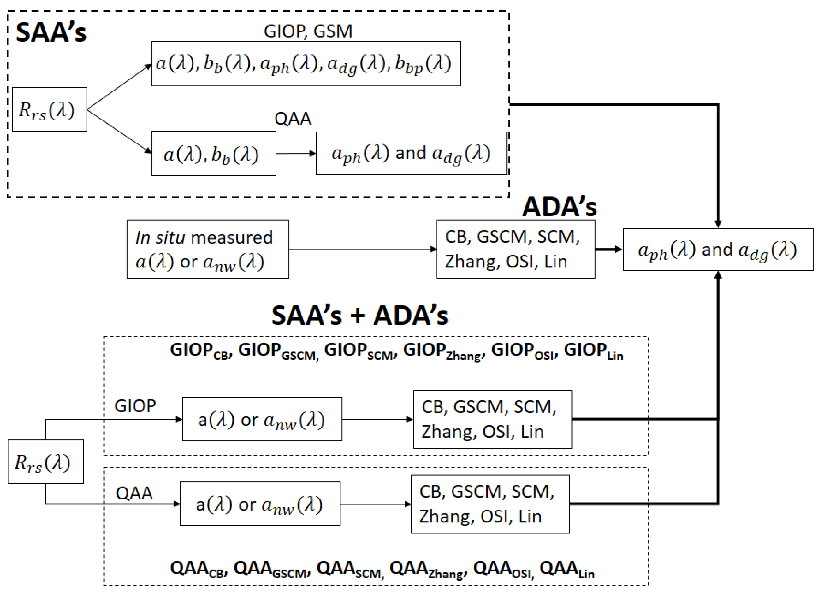
To achieve the above-mentioned objectives, six ADAs with different methodologies and three operational SAAs are used. Figure 1 shows the systemic methodology of the study.
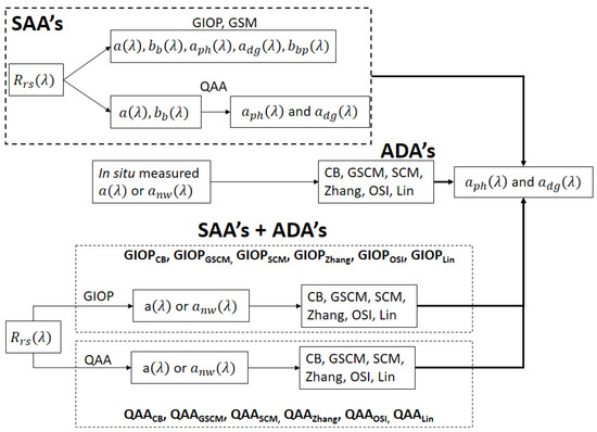
Figure 1.
Semi-analytical Algorithms (SAAs) use and provide bulk and subcomponent IOPs as outputs. Absorption decomposition algorithms (ADAs) derive absorption subcomponents from total or non-water absorption coefficient. In hybrid SAAADA models, from an SAA is input to ADA to derive absorption subcomponents.
2.1. Absorption Decomposition Algorithms (ADAs)
ADAs use or as input to provide absorption subcomponents as outputs. The six ADA’s used in this study, are (1) Ciotti and Bricaud’s model [18] (2) Stacked Constraints Model (SCM) [1] (3) Lin’s model [16] (4) Generalized Stacked Constrained Model (GSCM) [17] (5) Optical Signature Inversion (OSI) method [15] and (6) Zhang’s model [20]. The input variables and outputs provided by each ADA are summarized in Table 1.

Table 1.
Absorption spectrum decomposition algorithms used in the study with outputs. “X” indicates the outputs provided by each algorithm.
The first ADA is the non-linear optimization method by Ciotti and Bricaud (2006) [18] based on the inversion technique by Roesler and Perry (1995) [23]. In this method, the phytoplankton light absorption was modelled according to the spectral mixing model that uses normalized shapes for pico- and micro- plankton and a size parameter, [18]. An exponentially decreasing slope model is used to model . The three parameters optimized in this model are and . To find optimal values of the three parameters that minimize the relative error between measured and modelled , MATLAB’s inbuilt routine of “fminsearch” is used. “fminsearch” uses Nelder–Mead simplex algorithm wherein the concept of a simplex is used. The algorithm takes series of steps to achieve the minimum of the objective function. At each step, the objective function is evaluated and the next step is taken to reduce the value of the objective function. The initial guess value of the variables should be chosen carefully based on the observed range of variability in parameters to avoid local minima entrapment. The initial guess values of the three variables are set to 0.5, 0.02 and 0.015 . More information about the “fminsearch” algorithm can be found at [24].
The SCM model partitions into absorption subcomponents based on the stacked-constraints approach. SCM model uses several inequality constraints derived using an extensive, quality-verified set of field data covering clear ocean to turbid coastal waters from low to high latitudes. SCM requires an input of at a minimum of six wavelengths of 412, 443, 490, 510, 555 and 670 nm. The model outputs an optimal and a range of feasible solutions of and . GSCM model is based on the SCM model and is capable of separating and using weakly restrictive assumptions about the component absorption coefficients. The shapes used to parameterize and were obtained from Chesapeake Bay, USA. GSCM requires an input of at a minimum of six wavelengths of 412, 443, 469, 490, 555, 670 nm. GSCM exhibited good performance in deriving absorption subcomponents from the Chesapeake Bay.
Lin’s model partitions three times to obtain absorption subcomponents along with respective slopes for each derived subcomponent. The eigenvectors used in this method are based on second-order polynomial fit obtained with data from NASA bio-Optical Marine Algorithm Dataset (NOMAD) and field samples from the Northern South China Sea (NSCS). Lin’s model was validated on an independent dataset derived from the Bermuda bio-Optics project.
The Optical Signature Inversion (OSI) method uses non-linear constrained least squares regression procedure to minimize the error between modelled and ac-9 measured . This model uses three normalized spectral phytoplankton curves [25] for modelling phytoplankton absorption and an exponential model to model NAP and CDOM absorption components. OSI method imposes constraints on CDOM exponential slope, phytoplankton absorption, CDOM and NAP absorption weights. Zhang’s model partitions in two steps. A kernel containing basis vectors of pico-, nano- and micro- plankton ([26]) and is created. An exponentially decreasing curve with a slope is used to model . The value is randomly varied in the range [0.004, 0.02] . The first step inverts a linear system of equations to retrieve phytoplankton size classes and from input . In the second step, the optimal that minimizes the error between modelled and measured is derived by implementing MATLAB’s “fminbnd” non-linear optimization scheme. “fminbnd’ finds the value of a single parameter of a function that minimizes the function on a bounded domain. This algorithm finds only one minimum, can only find minima based on one variable and operates only on one variable at a time. This algorithm is based on golden section search and parabolic interpolation. More information about the algorithm can be found at [27,28]. Since is the only variable to be optimized in the second step of the Zhang’s algorithm, the “fminbnd” function is used.
2.2. Semi-Analytical Algorithms (SAA)
To combine ADAs with SAAs, or derived from remote sensing reflectance using SAAs is necessary. Many SAAs were proposed in the past decade to derive the bulk IOPs either from measured or satellite-derived [8]. Three widely used and operational SAA’s, Generalized Inherent Optical Property (GIOP) framework [9], Garver–Siegel–Maritorena (GSM) algorithm [11] and the Quasi-Analytical Algorithm (QAA) [12,13,14] are used to derive or .
GSM was initially developed by Garver and Siegel (1997) [10] and later updated by Maritorena et al., 2002 [11]. It uses a bio-optical model parameterized by a chlorophyll-specific phytoplankton absorption coefficient (), and the slope of parameters derived from a global quasi-real dataset. A non-linear optimization scheme is employed to obtain optimal values of chlorophyll concentration [Chl], and that provide the least error between the modelled and measured values of . The retrieved values are considered valid based on the ranges, 0.01 < [Chl] <64 mg/m3, 0.0001 < < 2.0 m−1 and 0.0001 < < 0.1 m−1. Levenberg-Marquardt [29,30,31] optimization routine is used as the computational method of optimization.
The GIOP framework allows the user to construct multiple SAA’s with a different configuration at each run time. The configurable options in the GIOP framework are bidirectional reflectance distribution function (BRDF), type of computational method of inversion, eigenvector or representative shape vectors for the subcomponents, wavelength range, Raman scattering. The default configuration of GIOP uses a non-linear spectral optimization routine with the Levenberg–Marquardt method as an optimization technique. The default configuration for GIOP uses: a specific absorption model for phytoplankton from Bricaud et al. (1995) [32] normalized by 0.055 m−2 (mg C)−1; the slope of particulate backscattering model from QAA; exponential spectral shape model for modelling with fixed slope, of 0.018 nm−1. The outputs of the GIOP model are Chlorophyll and spectral IOPs. All retrieved IOPs falling in between −0.005 and 5 m−1 are considered valid. The derived IOPs are considered invalid if the reconstructed differs from the observed by more than 33%.
QAA is an algebraic algorithm that uses empirical, semi-analytical and analytical equations in a step-wise manner to derive bulk and subcomponent IOPs from of optically deep waters. In the first step, is derived from and in the second, is decomposed into subcomponents, and .
The hybrid models are formulated by combining SAAs and ADAs. The first step of hybrid models involve deriving from using SAAs. In the second step, the SAA model-derived is used as input to various ADAs to derive absorption subcomponents (Figure 1). The hybrid models are indicated by the notation SAAADA. For example, if derived from GIOP is used as input to GSCM model, the notation would be GIOPGSCM.
2.3. Statistical Indicators
The mean absolute percentage error (MAPE), root mean squared error (RMSE) in log scale and N% are used to evaluate the performance of various models in deriving IOPs since the datasets cover a wide range of optical properties.
where and are measured and modelled absorption coefficients, N is the total number of valid measured absorption coefficients. The retrieved absorption subcomponents are valid when they lie in the range of 0.0001 and 5 m−1. The average spectral MAPE and RMSElog10 calculated as the mean of MAPE and RMSElog10 values at all wavelengths are used as additional measures in comparisons of models.
2.4. Datasets
Four datasets covering a wide range of optical properties are used to evaluate the performance of ADAs, SAAs and SAAADA models (Table 2). The variation in and corresponding subcomponent IOPs for the four datasets is presented in Figure 2. The first dataset is a simulated dataset created as a part of the International Ocean-Colour Coordinating Group (IOCCG)’s Algorithm Working Group [33]. This dataset was generated using Hydrolight [34] using known concentrations of IOP inputs covering a wide range of optical properties observed in natural waters. This dataset consists of 500 simulated along with corresponding spectral absorption coefficient of and in 400–800 nm wavelength range with 10 nm spacing. For this study, the spectral IOPs and at six wavelengths of 412, 443, 490, 510, 555 and 670 nm present in most of the ocean colour sensors were used. This dataset is hereafter referred to as the IOCCG dataset.

Table 2.
Datasets used in the study with available wavelengths and ranges of absorption due to phytoplankton at 443 nm and coloured detrital matter
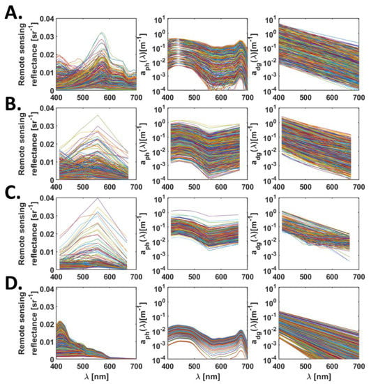
Figure 2.
Variation in remote sensing reflectance, absorption due to phytoplankton and absorption due to coloured detrital matter observed in (A) IOCCG, (B) GB, (C) CCRR and (D) the Red Sea datasets.
The second dataset corresponds to a subset of the global bio-optical in situ dataset curated as a part of the European Space Agency’s Ocean Colour Climate Change Initiative (OC-CCI) [35]. This dataset consists of and the IOPs and at six wavelengths (same as IOCCG) for 860 stations acquired over a wide range of environments covering clear to turbid ocean waters. This dataset is hereafter referred to as the GB dataset.
For development and evaluation of algorithms for coastal water quality, Coast Colour Round Robin (CCRR) project brought together an in situ dataset with sampling locations at 11 coastal sites spread around the globe [36]. The third dataset is a subset of the in situ dataset and consists of 348 spectral and corresponding IOPs of and at six wavelengths 412, 443, 490, 510, 555 and 665nm. Most of the stations in this dataset are located along the coastal waters of Southern California and Florida, USA. This dataset is hereafter referred to as the CCRR dataset. The locations of stations in GB and CCRR datasets are shown in Figure 3.
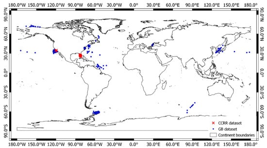
Figure 3.
Locations of Stations in GB datasets (Blue Circles) and CCRR dataset (Red Cross).
The fourth dataset corresponds to a simulated dataset generated using Hydrolight with inputs of known concentrations of bio-optical parameters in the Red sea oligotrophic waters [37]. Briefly, this dataset consists of 5000 random spectra of and spectral IOPs of in 350–800 nm wavelength range with 5 nm spacing. The ranges of chlorophyll and non-algal particulate material used in simulations are 0.01–0.50 mg/m3 and 0–0.1 g/m3. The slopes, and are varied from 0.01–0.03 nm−1 and 0.007–0.021 nm−1. Pure water absorption coefficients are taken from Pope and Fry (1997) [38]. This dataset is hereafter referred to as the Red Sea dataset.
In IOCCG and the Red Sea simulated datasets, the input IOPs are generated using random numbers and equations for the absorption subcomponents. These IOPs are used as input to Hydrolight to simulate . In the case of GB and CCRR datasets, both IOPs and are concurrently measured in situ. While in situ measured datasets are crucial to evaluate model performance in real-world scenarios, the number of data points and their extent may not cover the entire variability observable in natural waters. Hence, simulated datasets that cover additional natural variability in waters not observed in the in situ datasets are required. Therefore, it is crucial to include both simulated and measured datasets in evaluating model performance.
3. Results
Firstly, the performance of the existing global semi-analytical algorithms, GIOP, GSM and QAA in deriving from measured or simulated from the four datasets is evaluated. This step is critical for quantifying the errors in the SAA model-derived or , which are then used as inputs to the second step of hybrid SAAADA models. The second comparison involves evaluating the performance of each ADA in deriving absorption subcomponents using measured . Evaluating the performance of ADAs using measured demonstrates their capability in partitioning in ideal conditions, i.e., negligible or minimal errors in the input. The ADAs capable of providing absorption subcomponents with lower errors are used for combining with SAAs to form SAAADA models. The SAAADA models are then evaluated for deriving absorption subcomponents from and are compared with existing global SAAs.
3.1. Performance Evaluation of Semi-Analytical Algorithms in the Retrieval of
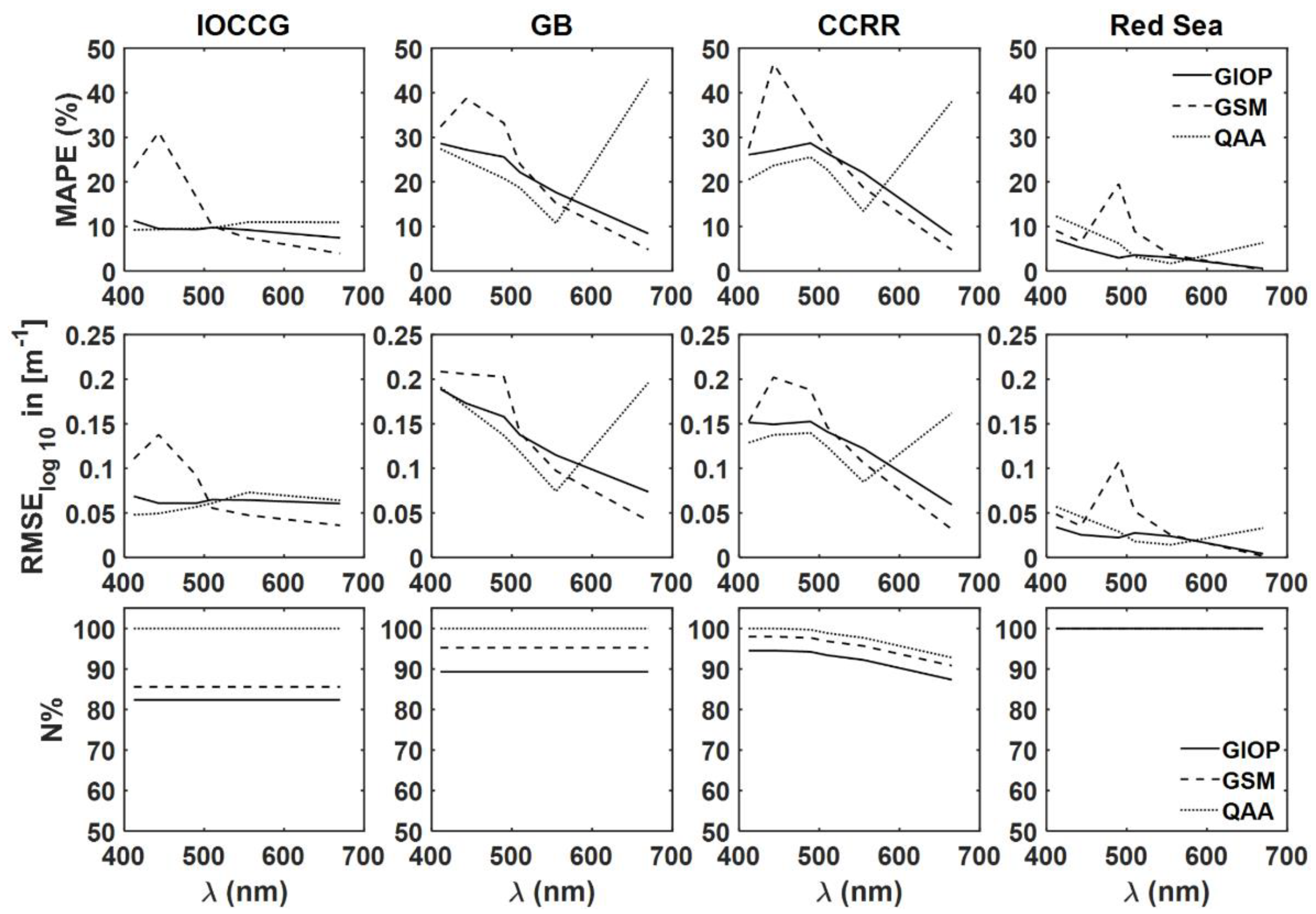
The three existing operational SAAs, i.e., GIOP with the default configuration, QAA and GSM, use measured or simulated as input to estimate the bulk and subcomponent IOPs as outputs (Figure 4). For IOCCG and the Red Sea simulated datasets, it is observed that the MAPE values for GIOP and QAA derived at all selected wavelengths are less than 15%. For the GSM model, the MAPE values lie in the range of 5–30% and 2–20% for IOCCG and the Red Sea datasets. Higher MAPE in the derived is observed at blue wavelengths (443 nm) for the IOCCG dataset and green wavelengths (490 nm) for the Red Sea dataset.
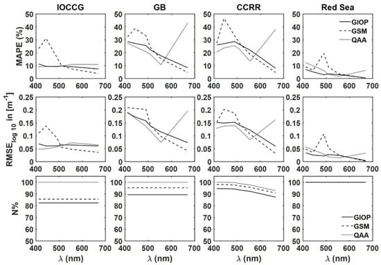
Figure 4.
Comparing GIOP, GSM and QAA algorithms in the retrieval of from measured or simulated spectral remote sensing reflectance, from IOCCG, GB, CCRR and Red Sea datasets.
In both GB and CCRR datasets, the GSM model exhibited higher MAPE values in the blue-green region in the range of 20–50% and exhibited a decreasing trend towards red wavelengths. The MAPE values for QAA-derived from GB and CCRR datasets are higher at 412 nm and decreased with an increase in wavelength till 555 nm; at 670 or 665 nm, the MAPE values reached ~40%. The MAPE and RMSElog10 values for GIOP algorithm derived for GB and CCRR datasets are higher at 412 nm and decrease with wavelength. Unlike QAA, higher errors were not observed for the derived a(670) or a(665) for GIOP or GSM models. As the present study focuses on the errors in SAA-derived , the total and particulate backscattering coefficients accuracy is not assessed. Compared with GIOP and QAA models, the GSM model resulted in relatively higher MAPE values for all four datasets. Hence, only GIOP and QAA model derived are used as input to the ADAs.
3.2. Performance Evaluation of ADAs in the Retrieval of Absorption Subcomponents from Measured
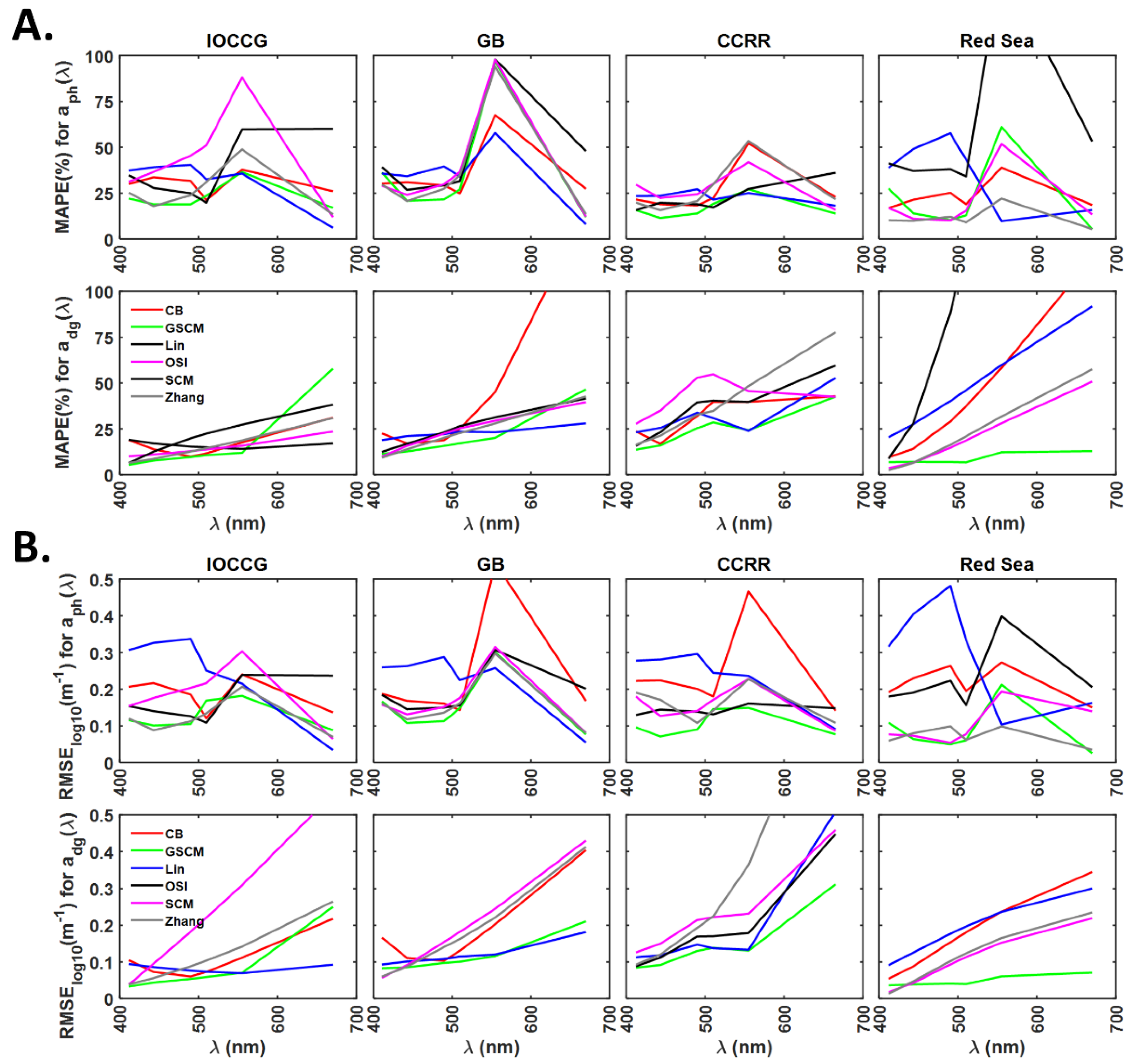
The performance of six ADAs are evaluated based on the errors observed in the derived and from . For the IOCCG dataset, and derived from all ADAs have the highest MAPE and RMSElog10 values than the rest of the wavelengths (Figure 5A). The MAPE values obtained for and from all ADAs at all wavelengths lie in the range of 5–88% and the average spectral MAPE in 22–44% (Figure 5A). The average spectral MAPE for derived from GSCM is the lowest (22%). The average spectral RMSElog10 values obtained for GSCM and Zhang models derived are lowest (0.122–0.126 ) among the ADAs. In the case of , average spectral MAPE values of all models, except SCM, lie in the range of 14–17%. GSCM and Lin model-derived obtained lowest average spectral RMSElog10 of 0.082–0.085 (Figure 5B). The N% for absorption subcomponents from all ADAs are always >80%, with GSCM exhibiting the lowest N% of 82% among all ADAs (Figure S1). Based on the observed errors, the order of performance of ADAs in deriving the absorption subcomponents from of IOCCG dataset is GSCM > Zhang > CB > Lin > OSI > SCM, where GSCM model-derived absorption subcomponents have lowest errors and SCM the highest.
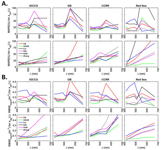
Figure 5.
Comparison of the six ADAs, CB, GSCM, Lin’s, OSI, SCM and Zhang’s, in deriving and from using statistical indicators (A). MAPE, (B). RMSE in log scale.
In the case of the GB dataset, average spectral MAPE values for from CB, GSCM, Zhang and Lin’s models are identical and vary from 34 to 36%. OSI model-derived exhibited the highest average spectral MAPE of 45%. In the case of , the average spectral MAPE values for GSCM and CB model-derived are the lowest (20%) and highest (45%). The average spectral MAPE values for derived from remaining models lie in the range of 22–25%. Based on MAPE and RMSElog10 errors (Figure 5A,B), the order of performance of ADAs is GSCM > (Zhang Lin) > SCM > (OSI CB).
MAPE values for the derived absorption subcomponents from all ADAs for the CCRR dataset lie in the range of 11–77%. GSCM model-derived and obtained the lowest average spectral MAPE values of 16% and 25%, respectively. The average spectral MAPE values for and from the remaining models lie in 23–27% and 31–43%, respectively. As observed in MAPE statistic, the lowest RMSElog10 values are obtained for GSCM derived and with average spectral RMSElog10 values of 0.104 and 0.147 , respectively. The order of performance of ADAs based on the error statistics for the derived absorption subcomponents is GSCM > (Lin OSI) > Zhang > SCM > CB.
In the case of the Red sea dataset, Zhang model-derived obtained the lowest average spectral MAPE value of 11% among all ADAs. Average spectral MAPE for from rest of the models lie in the range of 19–59%. In agreement with MAPE, the RMSElog10 values for Zhang’s model-derived are the lowest with an average spectral RMSElog10 of 0.072 . In the case of , GSCM model obtained the lowest average spectral MAPE of 9% and spectral RMSElog10 of 0.047 . Based on MAPE and RMSElog10 statistics obtained for both absorption subcomponents, the order of performance of ADAs for the Red Sea dataset is GSCM > Zhang > SCM > CB > Lin > OSI.
Error statistics computed for the derived absorption subcomponents from the four datasets show that the GSCM model performed better than all other ADAs with the lowest errors. After GSCM, lower errors were observed in Zhang’s model for IOCCG, GB and the Red Sea datasets. Hence, these two ADAs are selected for combining with SAAs of GIOP and QAA to form SAAADA models. As a special case, the CB model is also included as this model was evaluated previously [39] for studying spatio-temporal variations in phytoplankton size and coloured detrital matter at global and regional scales.
3.3. Hybrid Inversion Models for Deriving Absorption Subcomponents from Remote Sensing Reflectance
The six hybrid SAAADA models, GIOPCB, QAACB, GIOPGSCM, QAAGSCM, GIOPZhang and QAAZhang, are compared with GIOP and QAA using statistical indicators of MAPE, RMSElog10 and . As observed in the previous section, GIOP model-derived from the Red Sea dataset obtained the least average spectral MAPE value of 6%. In an ideal situation, derived from each SAA will have the least possible error. In such a case, assessing each ADA’s performance in waters with a wide range of optical variability is necessary for deriving accurate absorption subcomponents. Hence, an ideal case wherein the measured provided as input to each ADA to derive absorption subcomponents is included in each comparison. The comparison of remaining SAAADA models with SAAs is presented in Figures S3–S5 as Supplementary Information.
3.3.1. Performance Evaluation of Hybrid Models in Deriving
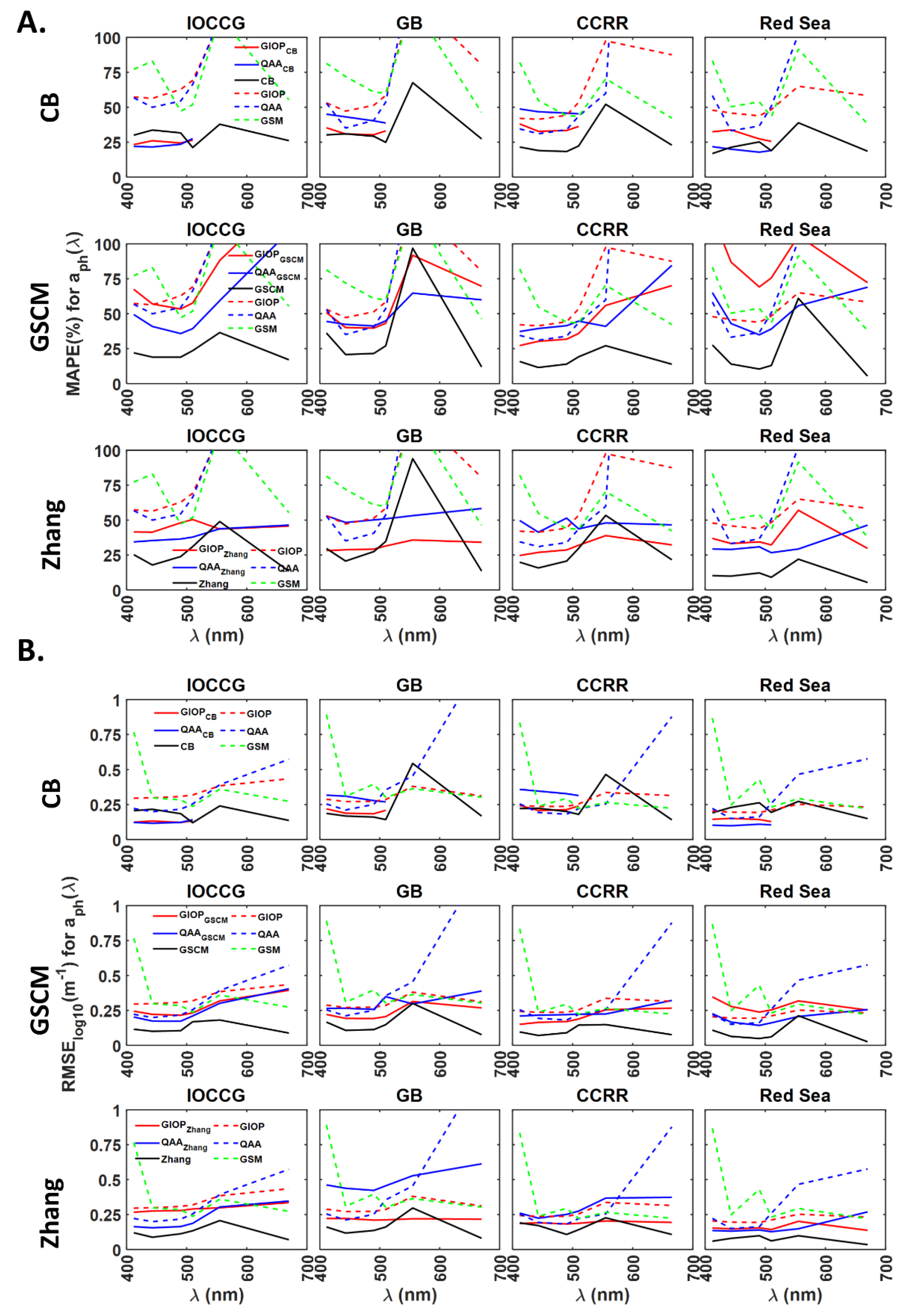
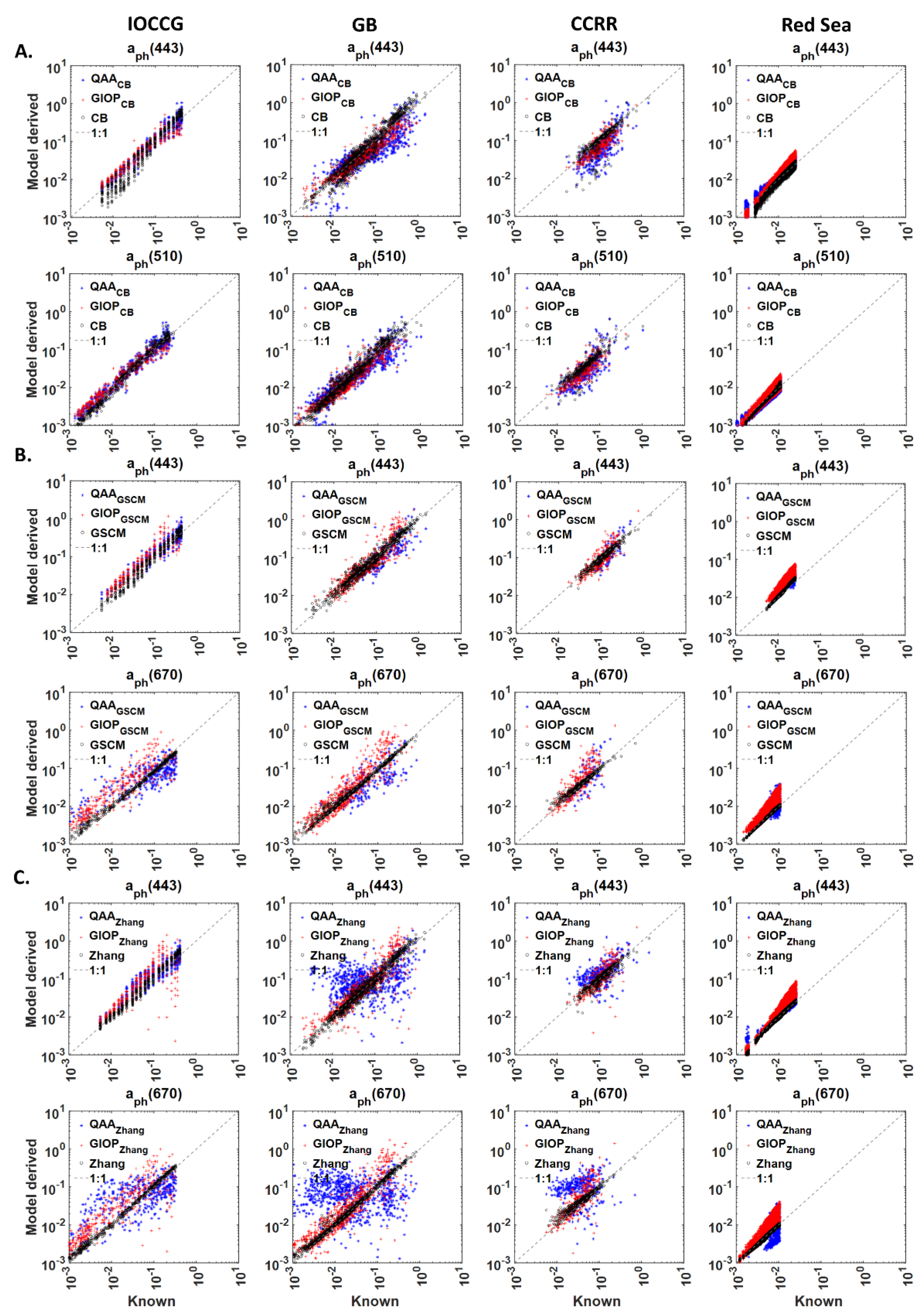
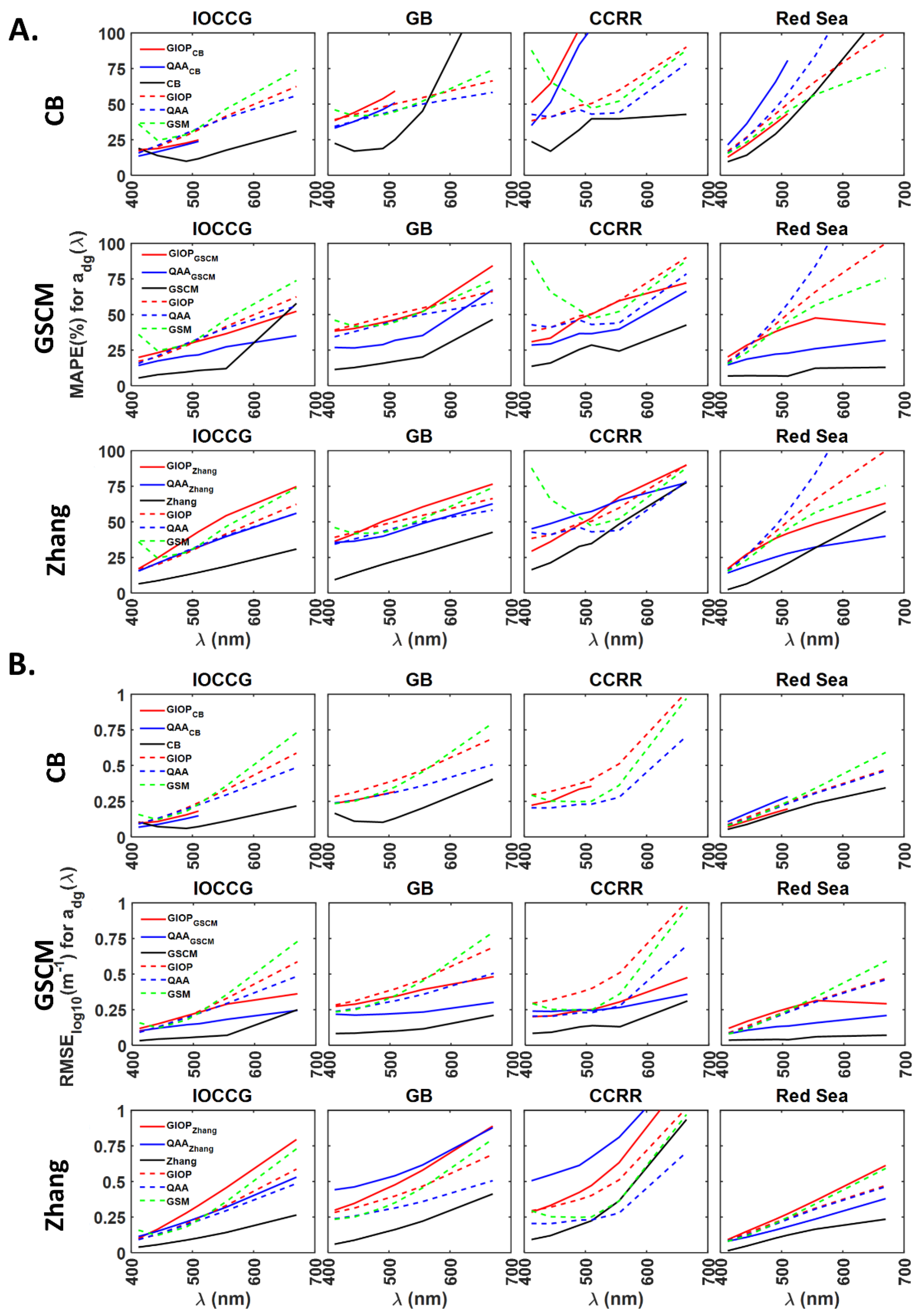
For the IOCCG dataset (Figure 6A, Row 1), GIOPCB and QAACB model-derived have 23–42% lower MAPE compared to GIOP and QAA models. Higher MAPE values were observed for for all the models. MAPE values for GIOPCB and QAACB derived are 6–11% lower compared to the CB model. For the GB dataset, MAPE values for GIOPCB and QAACB models derived are 4–25% lower than GIOP and QAA models. In the case of the CCRR dataset, GIOPCB model-derived obtained 4–17% lower MAPE compared to GIOP model-derived . For the Red Sea dataset, GIOPCB model-derived have 12–22% and 4–6% lower MAPE values compared to the GIOP model. Similarly, compared to the QAA model, MAPE values for from GIOPCB model are 1–25% and 2–14% lower. QAACB model-derived have 25–29% and 13–36% lower MAPE values than GIOP and QAA models. The validity of absorption subcomponents derived from GIOPCB and QAACB models varied in the range 82–100% (Figure S2A). These results indicate that only GIOPCB model performed better with lower errors than GIOP and QAA models for the Red Sea dataset. In the case of GB, CCRR and the Red Sea datasets, GIOPCB and QAACB model-derived absorption subcomponents obtained 1–34%, 11–70% and 1–43% higher MAPE values than the CB model. Absorption subcomponents derived from QAACB and GIOPCB models deviated less in simulated datasets than GB and CCRR datasets (Figure 7A).
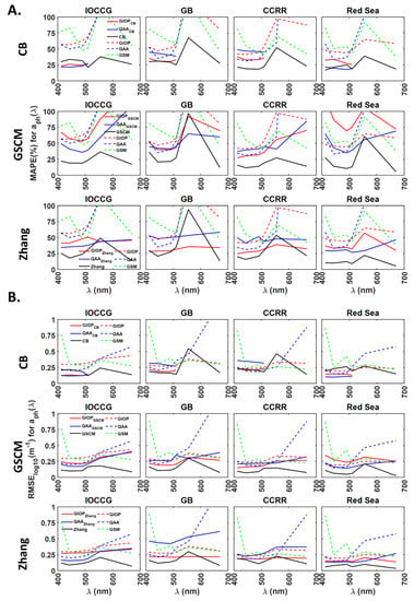
Figure 6.
Comparison of GIOPCB, QAACB, GIOPGSCM, QAAGSCM, GIOPZhang and QAAZhang models in deriving from of IOCCG, GB, CCRR and Red Sea datasets using (A). MAPE and (B). RMSE in log scale. Here, GIOPCB indicates that GIOP algorithm with default configuration is used to derive from of each of the four datasets. In the second step, the GIOP-derived is used as input to CB algorithm to obtain absorption subcomponents of and . The same procedure is used in GIOPZhang, QAAZhang, GIOPGSCM and QAAGSCM models. GIOP, QAA and GSM are the existing operational semi-analytical algorithms that use as input and provide absorption subcomponents as outputs. The CB, GSCM and Zhang’s models use spectral non-water absorption coefficient, as input to derive the absorption subcomponents.
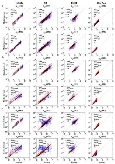
Figure 7.
Comparison of model-derived and known (measured or synthetic) values of the phytoplankton absorption coefficient, from (A). GIOPCB, QAACB and CB models at 443 and 510 nm, (B). GIOPGSCM, QAAGSCM and GSCM models at 443 and 670 nm, (C). QAAZhang, GIOPZhang and Zhang’s models at 443 and 670 nm. The hybrid models QAACB, QAAGSCM, QAAZhang, GIOPCB, GIOPGSCM and GIOPZhang models use , spectral remote sensing reflectance to derive absorption subcomponents. Blue dots and red plus indicate the hybrid models that use GIOP and QAA in the first step. The absorption decomposition algorithms, CB, GSCM and Zhang’s (Black circles) models, use , spectral non-water absorption coefficient to derive the absorption subcomponents, is the wavelength. The inputs for the models, i.e., and are taken from the four datasets, IOCCG, GB, CCRR and the Red Sea. The 1:1 relationship is shown in a grey dotted line.
The average spectral MAPE value for derived from GIOPGSCM is ~7% less than GIOP for the IOCCG dataset. The average spectral MAPE values for GIOPGSCM and QAA are similar, with a difference of less than 1% (Figure 6A,B, Row 2). For the GB dataset, MAPE values for from GIOPGSCM are 2–15% and 2–10% less than GIOP and QAA models. Similarly, QAAGSCM derived obtained 4–13% and 1–8% lower MAPE values than GIOP and QAA models. Overall, for GB dataset, QAAGSCM model-derived absorption subcomponents are lower than GIOP and QAA models. The lower MAPE values can be a consequence of the lower N% of 19% observed for QAAGSCM derived , as compared to 90–100% valid retrievals of GIOP and QAA. GIOPGSCM derived absorption subcomponents also obtained a lower N% of 76% (Figure S2A). For the CCRR dataset, compared to GIOP and QAA-derived in 412–555 nm range, GIOPGSCM model obtained 14–41% and 2–7% lower MAPE values. QAAGSCM derived obtained 2–56% lower and 2–18% higher MAPE values than GIOP. The N% values obtained for both and derived from GIOPGSCM, QAAGSCM, GIOP and QAA models are 92%, 22%, 94% and 100%, respectively. These results imply that the lower MAPE values from the QAAGSCM model can be a consequence of the lowest N%, as witnessed in GB dataset.
In comparison with GIOP and QAA models, derived from GIOPZhang models obtained 6–18% lower MAPE values in 410–510 nm range for IOCCG dataset. GIOP and QAA-derived at 555 and 670 nm wavelengths have >100% MAPE; hence, they are excluded from the comparison (Row 3, Figure 6A,B). For the GB dataset, GIOPZhang model-derived in 412–510 nm range have 18–26% and 6–24% lower MAPE than GIOP and QAA models. QAAZhang model-derived obtained 1–7% lower MAPE values than GIOP and 1–9% higher MAPE values than QAA models. For the CCRR dataset, GIOPZhang model-derived obtained 14–58% and 4–20% lower MAPE than GIOP and QAA models. QAAZhang model-derived exhibited ~7% higher error in the 412–490nm range and 9–50% lower error in 510–670 nm compared to the GIOP model. Similarly, MAPE values for from QAAZhang are 10–17% higher than QAA-derived in 412–490 nm range. For the Red Sea dataset, MAPE values for GIOPZhang derived are 8–16% and 2–45% lower than GIOP and QAA. Similarly, QAAZhang model-derived in 412–555 nm range have 12–35% and 4–73% lower MAPE compared to the QAA model. In comparison with Zhang’s model, GIOPZhang and QAAZhang model-derived obtained 16–32% and 6–32% higher MAPE values. GIOPZhang model-derived from IOCCG, GB, CCRR and the Red Sea datasets have N% in the ranges of 37–64%, 63–79%, 65–87% and 59–79% (Figure S2A). Similarly, QAAZhang model-derived from IOCCG, GB, CCRR and the Red Sea datasets are 46–63%, 31–50%, 22–74% and 7–11% valid (Figure S2A). QAAZhang model-derived absorption subcomponents (Blue dots in Figure 7C) obtained higher biases than GIOPZhang (Red “+”) for all four datasets. Especially for the GB dataset, the deviations observed from the 1:1 line are higher for QAAZhang model-derived .
3.3.2. Performance Evaluation of Hybrid Models in Deriving
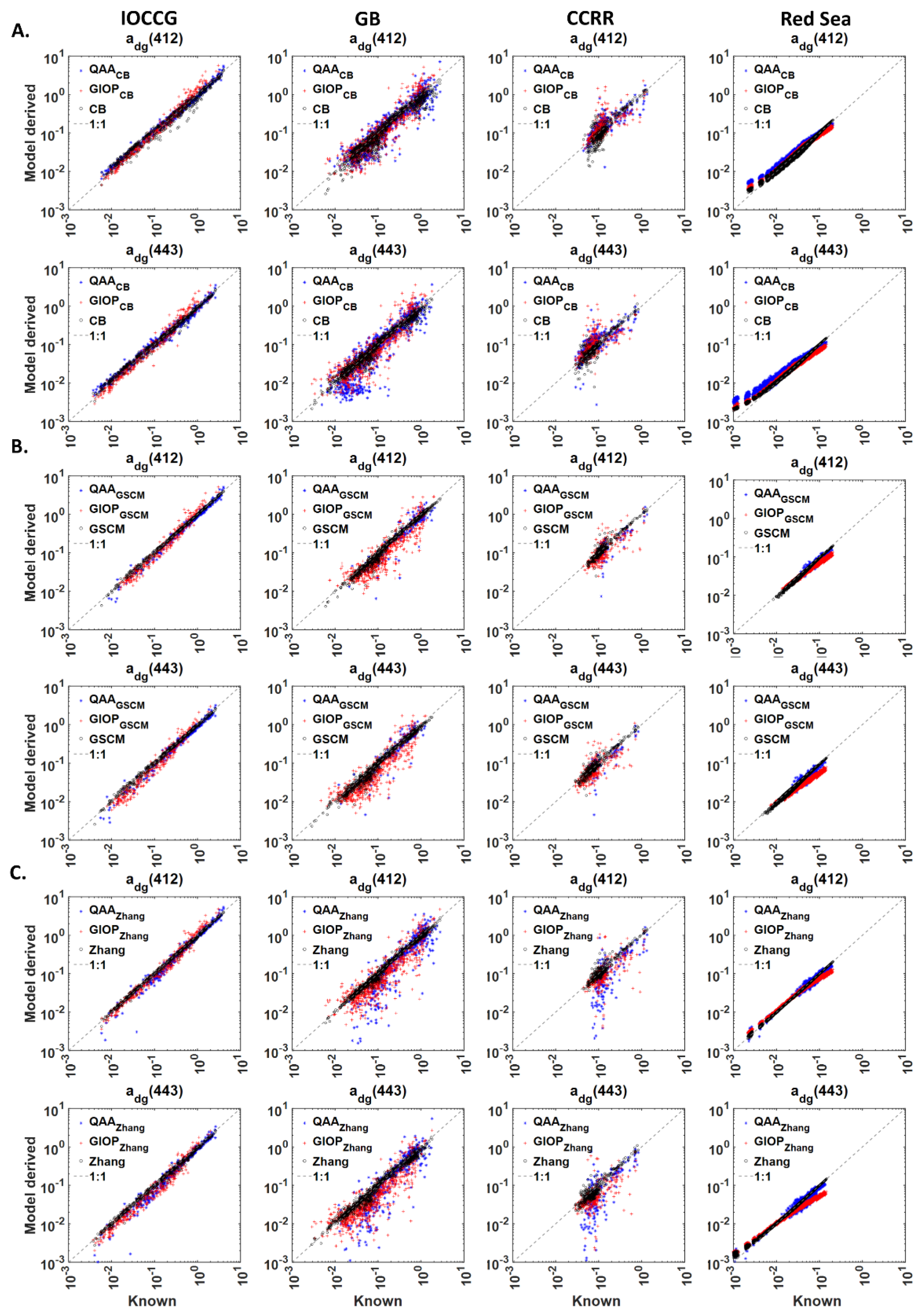
For the IOCCG dataset (Row 1, Figure 8A,B), GIOPCB and QAACB derived obtained 2–8% lower MAPE than GIOP and QAA models. Higher MAPE values were observed for for all the models. MAPE values for GIOPCB and QAACB model-derived are 2–13% higher than the CB model. For the GB dataset, the average spectral MAPE for derived from QAACB and GIOPCB models are 3% higher and 2% lower compared GIOP model. In comparison with QAA-derived , average spectral MAPE for QAACB and GIOPCB models-derived are 2% and 8% higher. For the Red Sea dataset, compared to the QAA model, MAPE values for from GIOPCB model are 2–14% lower. The errors for QAACB derived are 4–30% and 5–23% higher compared to GIOP and QAA models.
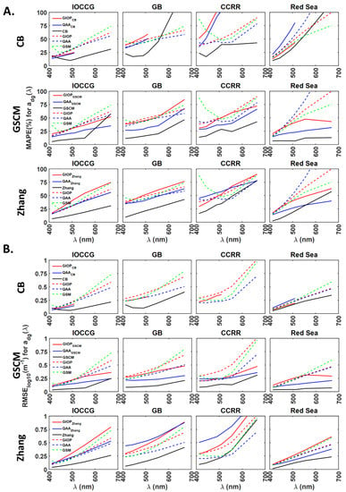
Figure 8.
Comparison of GIOPCB, QAACB, GIOPGSCM, QAAGSCM, GIOPZhang and QAAZhang models in deriving from of IOCCG, GB, CCRR and Red Sea datasets using (A). MAPE and (B). RMSE in log scale. Here, GIOPCB indicates that GIOP algorithm with default configuration is used to derive from of each of the four datasets. In the second step, the GIOP-derived is used as input to CB algorithm to obtain absorption subcomponents of and . The same procedure is used in GIOPZhang, QAAZhang, GIOPGSCM and QAAGSCM models. GIOP, QAA and GSM are the existing operational semi-analytical algorithms that use as input and provide absorption subcomponents as outputs. The CB, GSCM and Zhang’s models use spectral non-water absorption coefficient, as input to derive the absorption subcomponents.
The average spectral MAPE obtained for GIOPGSCM derived is ~2% lower than GIOP in the case of the IOCCG dataset. QAAGSCM derived obtained lower MAPE values in the range of 2–27% compared to GIOP and 1–20% lower MAPE than QAA (Row 2, Figure 8A). For the GB dataset (Row 2, Figure 8A), except at 670 nm, GIOPGSCM derived obtained lower MAPE values compared to GIOP and higher MAPE values compared to QAA. In 412–555 nm range, QAAGSCM derived obtained 12–19% lower MAPE values than QAA and 7–14% lower MAPE values than QAA. The lower MAPE values can be a consequence of the lower N% of 19% observed for QAAGSCM derived retrievals, as compared to 90–100% valid retrievals of GIOP and QAA. GIOPGSCM derived absorption subcomponents also obtained a lower N% of 76% (Row 2, Figure S2B). For the CCRR dataset, GIOPGSCM obtained ~5% lower average spectral MAPE compared to GIOP. QAAGSCM derived obtained 9–23% and 4–14% lower MAPE compared to GIOP and QAA models. The N% values obtained for derived from GIOPGSCM, QAAGSCM, GIOP and QAA models are 92%, 22%, 94% and 100%, respectively.
These results imply that the lower MAPE values from the QAAGSCM model can be a consequence of the lowest N%, as witnessed in GB dataset. MAPE values from QAAGSCM are 8–15%, 13–20%, 7–23% and 7–18% higher than GSCM. In addition, QAAGSCM and GIOPGSCM derived absorption subcomponents have higher biases than the GSCM model, as indicated by deviation from the 1:1 line. GIOPGSCM model-derived absorption subcomponents have higher biases (Figure 9B) compared to QAAGSCM for the Red Sea dataset, resulting in higher MAPE values (Row 2, Figure 8A).
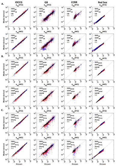
Figure 9.
Comparison of model-derived and known (measured or synthetic) values of the phytoplankton absorption coefficient, from (A). GIOPCB, QAACB and CB models at 443 and 510 nm, (B). GIOPGSCM, QAAGSCM and GSCM models at 443 and 670 nm, (C). QAAZhang, GIOPZhang and Zhang’s models at 443 and 670 nm. The hybrid models QAACB, QAAGSCM, QAAZhang, GIOPCB, GIOPGSCM and GIOPZhang models use , spectral remote sensing reflectance to derive absorption subcomponents. Blue dots and red plus indicate the hybrid models that use GIOP and QAA in the first step. The absorption decomposition algorithms, CB, GSCM and Zhang’s (Black circles) models, use , spectral non-water absorption coefficient to derive the absorption subcomponents, is the wavelength. The inputs for the models, i.e., and are taken from the four datasets, IOCCG, GB, CCRR and the Red Sea. The 1:1 relationship is shown in a grey dotted line.
GIOPZhang and QAAZhang derived MAPE values for from IOCCG dataset are higher or similar to QAA and GIOP models (Row 3, Figure 8A,B). For the GB dataset, QAAZhang obtained 3–8% lower MAPE values compared to GIOP and similar values to QAA. For the CCRR dataset, GIOPZhang derived obtained ~5% lower error compared to GIOP in 412–490 nm range and 2–7% higher in 510–670 nm range, indicating a similar overall error. QAAZhang model-derived have 5–6% and 2–21% higher MAPE compared to GIOP and QAA models. For the Red Sea dataset, the GIOPZhang model obtained 4–17% and 8–35% lower MAPE than GIOP and QAA in 490–555 nm. QAAZhang model-derived obtained 2–33% and 7–57% lower MAPE values than GIOP and QAA models. For the GIOPZhang model, the N% observed for IOCCG, GB, CCRR and the Red Sea datasets are 82–83%, 86–88%, 92–94% and 79–100% respectively (Row 3, Figure S2B). Similarly, QAAZhang model-derived from IOCCG, GB, CCRR and the Red Sea datasets obtained N% in the ranges of 75–73%, 43–50%, 44–47% and 10–11%, respectively. These results indicate that GIOPZhang model-derived absorption subcomponents are more valid compared to QAAZhang. However, the N% obtained for the GIOPZhang model is still lower than GIOP and QAA at all wavelengths and all datasets. GIOPZhang and QAAZhang model-derived obtained 10–43% and 8–25% higher MAPE than Zhang’s model. Overall, the QAAZhang model obtained lower MAPE values than GIOP and QAA in IOCCG, GB and the Red Sea datasets. However, the observed lower errors from QAAZhang can result from the lowest N% values obtained for absorption subcomponents.
The errors observed in absorption subcomponents derived from GIOPADA and QAAADA models are induced in two steps. First, from GIOP and QAA are not entirely error-free; hence, using erroneous induces additional error in GIOPADA and QAAADA model-derived absorption subcomponents. Second, ADA model-derived absorption subcomponents also are not error-free, implying that even if error-free are used as inputs, each ADA model derives absorption subcomponents with some error.
Summarizing the performance of hybrid SAAADA models, GIOPCB and QAACB model-derived absorption subcomponents obtained lower errors than GIOP and QAA only in the case of simulated datasets. GIOPGSCM model obtained lower errors for the derived absorption subcomponents in IOCCG, GB and CCRR datasets than GIOP and QAA models. Higher errors for the GIOPGSCM derived absorption subcomponents were observed in the case of the Red Sea dataset. A possible reason could be the Chesapeake Bay based parameterization of absorption subcomponents in the GSCM model, whereas the Red Sea dataset is mostly oligotrophic waters. For the Red Sea dataset, GIOPZhang model-derived absorption subcomponents achieved lower errors than GIOP and QAA models. Although QAAGSCM and QAAZhang derived absorption subcomponents obtained lower errors than GIOP and QAA, the lower errors can be attributed to lower N% values.
4. Discussion
4.1. Effect of Different Datasets on Model Performance
This paper focuses on developing hybrid inversion models to derive absorption subcomponents from remote sensing reflectance. Two simulated and two measured datasets covering a wide range of optical properties are used to facilitate intercomparison of the ADAs performance. GB dataset is the most extensive global dataset of in situ and concurrent IOPs. However, the distribution of the samples in the GB dataset is not equivalent to the global ocean. Eutrophic waters are over-represented in GB and oligotrophic waters are under-represented [35]. To compensate for this data gap, the Red Sea simulated dataset was used [37]. An ideal case of inter-comparison of models requires datasets exclusive of data used to parameterize the SAAs or ADAs. However, in the present study, it was difficult to assess the impact of IOCCG, GB and CCRR datasets on model performance, as these datasets influence most models to some extent. For example, QAA used in the present study uses an updated parameterization [14], wherein some empirical equations were based on the IOCCG and NOMAD, a significant contributor to the GB dataset used in the study [13]. Among the ADAs, the spectral shape model used in Lin’s model for modelling is based on a subset of NOMAD. Hence, independent datasets are required to assess the dataset’s influence on various models performance and in further evaluation of models.
An assumption related to in situ datasets is their closeness to the truth. In reality, in situ data may have some associated inherent errors. The use of robust quality control procedures to remove measurement outliers was adopted during the compilation of GB and CCRR datasets [35,36]. Measurements of absorption subcomponents and contain inherent errors depending on the type of method and instruments used [2]. Despite the application of the best available correction methods, measured using in situ absorption measuring instruments may contain a residual error of 20% or more. The magnitude of errors depend on wavelength region as well, with relatively higher errors observed in red and NIR wavelengths [40]. Quantifying the error associated with each variable at each wavelength with varying uncertainty levels is a tedious task. Future efforts to compile in situ observations with accompanying uncertainties are required. GB and CCRR datasets are in situ datasets, wherein the error associated with can be small as compared to satellite-derived . The performance of SAAs and ADAs may vary when data with higher levels of noise is used.
4.2. Applicability of Existing ADAs in Partitioning
Each ADA used in the study was designed for a specific purpose, as indicated by the different outputs they provide (Table 1). Each ADA’s advantages and disadvantages are dependent to a certain degree on the methodology, spectral shape models used and wavelengths. The performance of each ADA and the hybrid inversion methods developed using these ADAs are dependent on these factors. For example, the CB model provides , a parameter useful to spatio-temporal patterns of phytoplankton size at a global level [39]. Zhang’s model provides pico-, nano- and micro-plankton size classes useful to study phytoplankton diversity at global scales. Despite this, some of the ADAs are not devoid of limitations. CB model requires Chlorophyll concentration as input. To avoid dependency on field-measured inputs, [Chl] is derived from Ocean Colour Chlorophyll-a empirical algorithms like OC4 [41,42]. However, ancillary inputs can be a source of error that may affect the algorithm’s performance [1,20]. The shape and magnitude of the phytoplankton absorption spectrum vary based on phytoplankton community size, species and other effects like pigment packaging and photodegradation. Use of a second-order polynomial equation as in Lin’s ADA to model may limit its variation in spectral shape and thus limits its representativeness. Secondly, Lin’s model generates two sets of and that are not identical, indicating an incomplete closure [17]. As observed from the results, OSI method exhibited higher errors for the derived absorption subcomponents. A possible reason could be its parameterization focused on application to coastal regions. Along with , also exhibit high variability in both shape and magnitude [43] in world’s oceans and use of strict assumptions such as a fixed shape model as in CB, Lin’s and Zhang’s models may limit the retrieval performance [1]. GSCM model was developed and validated with data from Chesapeake Bay only and its applicability in other aquatic environments needed to be studied.
4.3. Effect of SAA Methodology in Deriving from
Based on results from spectral plots (Figure 4), QAA model-derived has higher errors at 670 nm in the case of GB and CCRR datasets. GSM model exhibited higher errors in blue-green wavelengths for all datasets. For most Case-1 global waters, water absorption dominates at higher wavelengths, i.e., at 665 or 670 nm and above. As a result, or approaches zero. QAA is an algebraic approach that derives the IOPs at each wavelength from the corresponding at that wavelength. When the available magnitudes are smaller, the errors in deriving increase, there by the errors in . The results for QAA model-derived IOPs lie in accordance with another comparison study [44]. A possible reason for lower errors observed in GIOP model-derived at longer wavelengths can be attributed to the indirect method of calculating . In GIOP, is not directly derived from , instead, it is calculated as the sum of and . The values of absorption subcomponents are derived using and at a reference wavelength, typically 443 nm and associated spectral shape models. Hence, the absorption subcomponents and are inferred from at shorter wavelengths.
All ADAs obtained higher errors in deriving at 555 nm and exhibited an increase in error for the derived towards longer wavelengths (Figure 5). A similar trend is observed in absorption subcomponents derived from ADAs that use derived GIOP and QAA. Among various ADAs, the ADA models that use from QAA didn’t perform well as compared to using from GIOP (Figure 6 and Figure 8).
4.4. Validity of the Derived Absorption Subcompnents and Statistical Indicator Selection
The range of absorption subcomponents used in the present study varies by more than three orders of range. For example for GB dataset varies in the range of 0.001–0.8199 . If most of the model-retrieved values are biased and deviate from the actual values, the observed MAPE value increases. Higher MAPE values, i.e., >100% were obtained for few models at 670 or 665 nm. The preliminary reason for such discrepancy in the model-derived value as compared to the actual value is as follows. The absorption due to pure water at these longer wavelengths (red and NearInfrared) is higher compared to its absorption at blue-green wavelengths. Thereby, the magnitudes of the absorption coefficients of subcomponents at longer wavelengths is very low. Deriving accurate absorption coefficients of subcomponents with smaller magnitudes at these longer wavelengths is particularly difficult. Similar higher errors in the derived absorption subcomponents were reported in previous studies [1]. To reduce the effect of such high spurious MAPE values on the entire model performance, the longer wavelengths are omitted. Further, to perform a proper comparison, the spurious MAPE values are removed from all the models in the comparison wherever necessary.
In most of the cases, the N% values obtained for various model-derived absorption subcomponents are greater than 75%. This statistic is important to find the model that is capable of deriving a maximum number of valid retrievals. Although, the present study deals with in situ and simulated data only, the proposed hybrid models can be applied to satellite data in further study. In the case of satellite datasets, the model’s ability to derive a maximum number of valid absorption subcomponents is crucial. The N% statistic at a wavelength depends on a numerous factors like type of methodology used in partitioning, errors present in the at the wavelength, magnitude of the absorption subcomponents etc. Except in longer wavelengths, the N% at blue-green wavelengths are nearly the same for all model-derived absorption subcomponents.
The performance of GSCM and Zhang’s model-based hybrid inversion approaches are better than other models because of the following reasons: 1. the spectral library of the GSCM model includes several measured distinct shapes for the absorption subcomponents, unlike other ADA’s wherein a modelled shape is used; 2. Zhang’s model provides more flexibility by allowing the model to choose optimal contributions of pico-, nano- and microplankton.
The present study may further be extended by deriving Chl from the derived or directly from . GIOP and GSM models in the SAA’s and Zhang’s ADA model only provide Chl as output and the rest of the models provide as outputs. Although Chl can be derived from using and Chl relationships, the errors would be higher because of two reasons. First, derived from SAAADA models are affected by errors in datasets and methodology adopted in SAA and ADA. Second, using a and Chl relationship with erroneous input of , may further induce additional errors in the derived Chl. Hence, this step is not pursued further.
5. Conclusions
Absorption decomposition algorithms partition the total absorption coefficient or non-water absorption coefficient into absorption subcomponents. Comparing the existing ADAs is essential to suggest an ADA capable of deriving absorption subcomponents over a wide range of waters. Based on the motive for partitioning , the output variables and methods vary for each ADA. The and are two standard outputs from the six ADAs, so this study focuses on comparing the models based on these two retrievals. Similar to CB and GSCM models, other ADAs need to be assessed for their applicability to remote sensing applications, i.e., the derivation of absorption subcomponents from . The purpose of the present study is to formulate and evaluate the performance of hybrid approaches that combine SAAs and ADAs to derive absorption subcomponents from both measured and SAA-derived . Among the six ADAs, GSCM and Zhang’s models had lower errors for the derived absorption subcomponents from measured . Similarly, GIOP and QAA algorithms obtained lower errors at most wavelengths in deriving from . Hence, from these two algorithms is used as inputs to GSCM, Zhang and CB models to formulate SAAADA hybrid models to derive absorption subcomponents from . Based on the statistical comparison, GIOPGSCM model-derived absorption subcomponents obtained lower errors than GIOP and QAA models for IOCCG, CCRR and GB datasets. In the Red Sea dataset, GIOPZhang model-derived absorption subcomponents obtained lower errors than GIOP and QAA models. Therefore, the hybrid models proposed in this study have shown better retrieval accuracy than the original semi-analytical inversion models. Uncertainties associated with the model performance and its dependency on datasets are discussed. More independent in situ datasets are required to evaluate the performance of models and quantify errors associated with in situ data.
Supplementary Materials
The following are available online at https://www.mdpi.com/article/10.3390/rs13091726/s1, Figure S1: Comparison of the six ADAs, CB, GSCM, Lin’s, OSI, SCM and Zhang’s in deriving and from using N%. Figure S2: Comparison of GIOPCB, QAACB, GIOPGSCM, QAAGSCM, GIOPZhang and QAAZhang models in deriving absorption subcomponents, (A). and (B). from of IOCCG, GB, CCRR and Red Sea datasets using N%. Here, GIOPCB indicates that GIOP algorithm with default configuration is used to derive from of each of the four datasets. In the second step, the GIOP-derived is used as input to CB algorithm to obtain absorption subcomponents of and . The GIOP, QAA and GSM are the existing operational semi-analytical algorithms that use as input and provide absorption subcomponents as outputs. The CB model uses spectral non-water absorption coefficient, as input to derive the absorption subcomponents. Figure S3: Comparison of GIOPLin and QAALin models in deriving absorption subcomponents, and from of IOCCG, GB, CCRR and Red Sea datasets using (A). MAPE (B). RMSElog10 and (C). N% statistics. Here GIOPLin indicates that GIOP algorithm with default configuration is used to derive from of each of the four datasets. In the second step, the GIOP-derived is used as input to Lin’s model to obtain absorption subcomponents of and .The GIOP, QAA and GSM are the existing operational semi-analytical algorithms that use as input and provide absorption subcomponents as outputs. Lin’s model uses spectral non-water absorption coefficient, as input to derive the absorption subcomponents. Figure S4: Comparison of GIOPSCM and QAASCM models in deriving absorption subcomponents, and from of IOCCG, GB, CCRR and Red Sea datasets using (A). MAPE (B). RMSElog10 and (C). N% statistics. Here GIOPSCM indicates that GIOP algorithm with default configuration is used to derive from of each of the four datasets. In the second step, the GIOP-derived is used as input to SCM model to obtain absorption subcomponents of and .The GIOP, QAA and GSM are the existing operational semi-analytical algorithms that use as input and provide absorption subcomponents as outputs. SCM model uses spectral non-water absorption coefficient, as input to derive the absorption subcomponents. Figure S5: Comparison of GIOPOSI and QAAOSI models in deriving absorption subcomponents, and from of IOCCG, GB, CCRR and Red Sea datasets using (A). MAPE (B). RMSElog10 and (C). N% statistics. Here GIOPOSI indicates that GIOP algorithm with default configuration is used to derive from of each of the four datasets. In the second step, the GIOP-derived is used as input to Lin’s model to obtain absorption subcomponents of and .The GIOP, QAA and GSM are the existing operational semi-analytical algorithms that use as input and provide absorption subcomponents as outputs.
Schofield’s OSI model uses spectral non-water absorption coefficient, as input to
derive the absorption subcomponents.
Author Contributions
Conceptualization, S.K. and S.P.T.; methodology, S.K. and S.P.T.; software, S.S.G.; validation, S.K. and S.P.T.; formal analysis, S.K.; investigation, S.K. and S.P.T.; resources, S.S.G. and S.P.T.; data curation, S.K. and S.P.T.; writing—original draft preparation, S.K.; writing—review and editing, S.K., S.P.T. and S.S.G.; visualization, S.K.; supervision, S.P.T. and S.S.G.; project administration, S.P.T. and S.S.G.; funding acquisition, S.P.T. and S.S.G. All authors have read and agreed to the published version of the manuscript.
Funding
This research received no external funding.
Data Availability Statement
The IOCCG dataset used is available at https://ioccg.org/resources/data/ (accessed on 9 December 2020). Similarly, GB and CCRR datasets are publicly available at https://doi.pangaea.de/10.1594/PANGAEA.854832 (accessed on 9 December 2020) and https://doi.pangaea.de/10.1594/PANGAEA.841952 (accessed on 9 December 2020). The codes for GSM and QAA models are available at https://ioccg.org/resources/software/ (accessed on 9 December 2020). The codes for Lin’s, Zhang’s, CB and OSI models were written in MATLAB as per the model description.
Acknowledgments
The authors would like to thank the Indian Institute of Technology Bombay and King Fahd University of Petroleum & Minerals for overall support to complete the research study. The authors are thankful to Guangming Zheng for providing us with the codes for GSCM and SCM models. We thank all the researchers, institutions and organizations responsible for making the GB, IOCCG and CCRR datasets publicly available.
Conflicts of Interest
The authors declare no conflict of interest
References
- Zheng, G.; Stramski, D. A model based on stacked-constraints approach for partitioning the light absorption coefficient of seawater into phytoplankton and non-phytoplankton components. J. Geophys. Res. Ocean. 2013, 118, 2155–2174. [Google Scholar] [CrossRef]
- Twardowski, M.S.; Rottgers, R.; Stramski, D. The Absorption Coefficient, An Overview. In Ocean Optics & Biogeochemistry Protocols for Satellite Ocean Colour Sensor Validation; International Ocean Color Coordinating Group (IOCCG) Report 2018; Bedford Institute of Oceanography: Dartmouth, NS, Canada, 2018; Chapter 1; pp. 1–15. [Google Scholar]
- WET Labs. ac Meter Protocol Document; WET Labs, Inc.: Philomath, Oregon, 2011. [Google Scholar]
- Freeman, S. Calibration and Data Processing of ACS Device; NASA GSFC: Greenbelt, MD, USA, 2012.
- Dana, D.R.; Maffione, R.A. A New Hyperspectral Spherical-Cavity Absorption Meter. In Proceedings of the AGU Ocean Sciences Meeting, Honolulu, HI, USA, 20–24 February 2006; pp. 1–13. [Google Scholar]
- Röttgers, R.; Häse, C.; Doerffer, R. Determination of the particulate absorption of microalgae using a point-source integrating-cavity absorption meter: Verification with a photometric technique, improvements for pigment bleaching, and correction for chlorophyll fluorescence. Limnol. Oceanogr. Methods 2007, 5. [Google Scholar] [CrossRef]
- Mobley, C.D. Light and Water: Radiative Transfer in Natural Waters; Academic Press: Cambridge, MA, USA, 1994. [Google Scholar]
- Werdell, P.J.; McKinna, L.I.W.; Boss, E.; Ackleson, S.G.; Craig, S.E.; Gregg, W.W.; Lee, Z.; Maritorena, S.; Roesler, C.S.; Rousseaux, C.S.; et al. An overview of approaches and challenges for retrieving marine inherent optical properties from ocean color remote sensing. Prog. Oceanogr. 2018, 160, 186–212. [Google Scholar] [CrossRef] [PubMed]
- Werdell, P.J.; Franz, B.A.; Bailey, S.W.; Feldman, G.C.; Boss, E.; Brando, V.E.; Dowell, M.; Hirata, T.; Lavender, S.J.; Lee, Z.; et al. Generalized ocean color inversion model for retrieving marine inherent optical properties. Appl. Opt. 2013, 52, 2019–2037. [Google Scholar] [CrossRef]
- Garver, S.A.; Siegel, D.A. Inherent optical property inversion of ocean color spectra and its biogeochemcial interpretation 1. Time series from the Sargasso Sea. J. Geophys. Res. 1997, 102, 18607–18625. [Google Scholar] [CrossRef]
- Maritorena, S.; Siegel, D.A.; Peterson, A.R. Optimization of a semianalytical ocean color model for global-scale application. Appl. Opt. 2002, 41, 2705–2714. [Google Scholar] [CrossRef]
- Lee, Z.; Carder, K.L.; Arnone, R.A. Deriving inherent optical properties from water color: A multiband quasi-analytical algorithm for optically deep waters. Appl. Opt. 2002, 41, 5755–5772. [Google Scholar] [CrossRef]
- Lee, Z.; Lubac, B.; Werdell, J.; Arnone, R. An Update of the Quasi-Analytical Algorithm (QAA-V5). Available online: https://www.researchgate.net/publication/228416418_An_update_of_the_quasi-analytical_algorithm_QAA_v5 (accessed on 22 March 2021).
- Lee, Z. Update of the Quasi-Analytical Algorithm (QAA_v6). Available online: http://www.ioccg.org/groups/Software_OCA/QAA_v6_2014209.pdf (accessed on 22 March 2021).
- Schofield, O.; Bergmann, T.; Oliver, M.J.; Irwin, A.; Kirkpatrick, G.; Bissett, W.P.; Moline, M.A.; Orrico, C. Inversion of spectral absorption in the optically complex coastal waters of the Mid-Atlantic Bight. J. Geophys. Res. Ocean. 2004, 109. [Google Scholar] [CrossRef]
- Lin, J.; Cao, W.; Wang, G.; Hu, S. Approach for determining the contributions of phytoplankton, colored organic material, and nonalgal particles to the total spectral absorption in marine waters. Appl. Opt. 2013, 52, 4249–4257. [Google Scholar] [CrossRef]
- Zheng, G.; Stramski, D.; Digiacomo, P.M. A model for partitioning the light absorption coefficient of natural waters into phytoplankton, nonalgal particulate, and colored dissolved organic components: A case study for the Chesapeake Bay. J. Geophys. Res. Ocean. 2015, 120, 2601–2621. [Google Scholar] [CrossRef]
- Ciotti, A.M.; Bricaud, A. Retrievals of a size parameter for phytoplankton and spectral light absorption by colored detrital matter from water-leaving radiances at SeaWiFS channels in a continental shelf region off Brazil. Limnol. Oceanogr. Methods 2006, 4, 237–253. [Google Scholar] [CrossRef]
- Oubelkheir, K.; Claustre, H.; Bricaud, A.; Babin, M. Partitioning total spectral absorption in phytoplankton and colored detrital material contributions. Limnol. Oceanogr. Methods 2007, 5, 384–395. [Google Scholar] [CrossRef]
- Zhang, X.; Huot, Y.; Bricaud, A.; Sosik, H.M. Inversion of spectral absorption coefficients to infer phytoplankton size classes, chlorophyll concentration, and detrital matter. Appl. Opt. 2015, 54, 5805–5816. [Google Scholar] [CrossRef]
- Roesler, C.S.; Perry, M.J.; Carder, K.L. Modeling in situ phytoplankton absorption from total absorption spectra in productive inland marine waters. Limnol. Ocean. 1989, 34, 1510–1523. [Google Scholar] [CrossRef]
- Zheng, G.; Digiacomo, P.M. Remote sensing of chlorophyll—A in coastal waters based on the light absorption coefficient of phytoplankton. Remote Sens. Environ. 2017, 201, 331–341. [Google Scholar] [CrossRef]
- Roesler, C.S.; Perry, M.J. In situ phytoplankton absorption, fluorescence emission, and particulate backscattering spectra determined from reflectance. J. Geophys. Res. 1995, 100, 22767. [Google Scholar] [CrossRef]
- Lagarias, J.C.; Reeds, J.A.; Wright, M.H.; Wright, P.E. Convergence properties of the nelder-mead simplex method in low dimensions. SIAM J. Optim. 1998, 9, 112–147. [Google Scholar] [CrossRef]
- Johnsen, G.; Samset, O.; Granskog, L.; Sakshaug, E. In vivo absorption characteristics in 10 classes of bloom-forming phytoplankton—Taxonomic characteristics and responses to photoadaptation by means of discriminant and HPLC analysis. Mar. Ecol. Prog. Ser. 1994, 105, 149–158. [Google Scholar] [CrossRef]
- Uitz, J.; Huot, Y.; Bruyant, F.; Babin, M.; Claustre, H. Relating phytoplankton photophysiological properties to community structure on large scales. Limnol. Oceanogr. 2008, 53, 614–630. [Google Scholar]
- Forsythe, G.E. Computer Methods for Mathematical Computations, 1st ed.; Prentice Hall: Hoboken, NJ, USA, 1977; pp. 1–259. [Google Scholar]
- Brent, R.P. Algorithms for Minimization without Derivatives; Dover Books on Mathematics; Dover Publications: Mineola, NY, USA, 2013; ISBN 9780486143682. [Google Scholar]
- Levenberg, K. A Method for the Solution of Certain Non-Linear Problems in Least. Q. Appl. Math. 1944, 2, 164–168. [Google Scholar] [CrossRef]
- Marquardt, D.W. An Algorithm for Least-Squares Estimation of Nonlinear Parameters. J. Soc. Indust. Appl. Math. 1963, 11, 431–441. [Google Scholar] [CrossRef]
- Gavin, H.P. The Levenburg-Marqurdt Algorithm for Nonlinear Least Squares Curve-Fitting Problems; Duke University: Durham, NC, USA, 2019; pp. 1–19. [Google Scholar]
- Bricaud, A.; Babin, M.; Morel, A.; Claustre, H. Variability in the chlorophyll-specific absorption coefficients of natural phytoplankton: Analysis and parameterization phytoplankton. J. Geophys. Res. 1995, 100, 13321–13332. [Google Scholar] [CrossRef]
- IOCCG. Remote Sensing of Inherent Optical Properties: Fundamentals, Tests of Algorithms, and Applications; Lee, Z.-P., Ed.; Reports of the International Ocean Colour Coordinating Group; IOCCG: Dartmouth, NS, Canada, 2006; Volume 5. [Google Scholar]
- Mobley, C.D.; Sundman, L.K. Hydrolight 5.2 Users’ Guide. Available online: https://www.sequoiasci.com/wp-content/uploads/2013/07/HE52UsersGuide.pdf (accessed on 22 March 2021).
- Valente, A.; Sathyendranath, S.; Brotas, V.; Groom, S.; Grant, M.; Taberner, M.; Antoine, D.; Arnone, R.; Balch, W.M.; Barker, K.; et al. A compilation of global bio-optical in situ data for ocean-colour satellite applications. Earth Syst. Sci. Data 2016, 8, 235–252. [Google Scholar] [CrossRef]
- Nechad, B.; Ruddick, K.; Schroeder, T.; Oubelkheir, K.; Blondeau-Patissier, D.; Cherukuru, N.; Brando, V.; Dekker, A.; Clementson, L.; Banks, A.C.; et al. CoastColour Round Robin data sets: A database to evaluate the performance of algorithms for the retrieval of water quality parameters in coastal waters. Earth Syst. Sci. Data 2015, 7, 319–348. [Google Scholar] [CrossRef]
- Tiwari, S.P.; Sarma, Y.V.B.; Kurten, B.; Ouhssain, M.; Jones, B.H. An optical algorithm to estimate downwelling diffuse attenuation coefficient in the red sea. IEEE Trans. Geosci. Remote Sens. 2018, 56, 7174–7182. [Google Scholar] [CrossRef]
- Pope, R.M.; Fry, E.S. Absorption spectrum (380–700 nm) of pure water. II. Integrating cavity measurements. Appl. Opt. 1997, 36, 8710–8723. [Google Scholar] [CrossRef]
- Bricaud, A.; Ciotti, A.M.; Gentili, B. Spatial-temporal variations in phytoplankton size and colored detrital matter absorption at global and regional scales, as derived from twelve years of SeaWiFS data (1998–2009). Glob. Biogeochem. Cycles 2012, 26. [Google Scholar] [CrossRef]
- Stockley, N.D.; Röttgers, R.; McKee, D.; Lefering, I.; Sullivan, J.M.; Twardowski, M.S. Assessing uncertainties in scattering correction algorithms for reflective tube absorption measurements made with a WET Labs ac-9. Opt. Express 2017, 25, A1139–A1153. [Google Scholar] [CrossRef]
- O’Reilly, J.E.; Maritorena, S.; Mitchell, B.G.; Siegel, D.A.; Carder, K.L.; Garver, S.A.; Kahru, M.; McClain, C.R. Ocean color chlorophyll algorighms for SeaWiFS. J. Geophys. Res. 1998, 103, 24937–24953. [Google Scholar] [CrossRef]
- O’Reilly, J.E.; Werdell, P.J. Chlorophyll algorithms for ocean color sensors—OC4, OC5 & OC6. Remote Sens. Environ. 2019, 229, 32–47. [Google Scholar] [CrossRef] [PubMed]
- Twardowski, M.S.; Boss, E.; Sullivan, J.M.; Donaghay, P.L. Modeling the spectral shape of absorption by chromophoric dissolved organic matter. Mar. Chem. 2004, 89, 69–88. [Google Scholar] [CrossRef]
- Brewin, R.J.W.; Sathyendranath, S.; Müller, D.; Brockmann, C.; Deschamps, P.Y.; Devred, E.; Doerffer, R.; Fomferra, N.; Franz, B.; Grant, M.; et al. The Ocean Colour Climate Change Initiative: III. A round-robin comparison on in-water bio-optical algorithms. Remote Sens. Environ. 2015, 162, 271–294. [Google Scholar] [CrossRef]
Publisher’s Note: MDPI stays neutral with regard to jurisdictional claims in published maps and institutional affiliations. |
© 2021 by the authors. Licensee MDPI, Basel, Switzerland. This article is an open access article distributed under the terms and conditions of the Creative Commons Attribution (CC BY) license (https://creativecommons.org/licenses/by/4.0/).

