Abstract
The glaciers in the Sawir Mountains are an important freshwater resource, and glaciers have been experiencing a continuing retreat over the past few decades. However, studies on detailed glacier mass changes are currently sparse. Here, we present the high-precision evolution of annual surface elevation and geodetic mass changes in the ablation area of the Muz Taw Glacier (Sawir Mountains, China) over the latest three consecutive mass-balance years (2017–2020) based on multi-temporal terrestrial geodetic surveys. Our results revealed clearly surface lowering and negative geodetic mass changes, and the spatial changing patterns were generally similar for the three periods with the most negative surface lowering (approximately −5.0 to −4.0 m a−1) around the glacier terminus. The gradient of altitudinal elevation changes was commonly steep at the low elevations and gentle in the upper-elevation parts, and reduced surface lowering was observed at the glacier terminus. Resulting emergence velocities ranged from 0.11 to 0.86 m a−1 with pronounced spatial variability, which was mainly controlled by surface slope, ice thickness, and the movement of tributary glaciers. Meanwhile, emergence velocities slightly compensated the surface ablation at the ablation area with a proportion of 14.9%, and dynamic thickening had small contributions to glacier surface evolution. Limited annual precipitation and glacier accumulation may result in these weak contributions. Higher-resolution surveys at the seasonal and monthly scales are required to get insight into the mass balance processes and their mechanism.
1. Introduction
Glacier mass balance is known to be one the most direct and immediate indicators of climate variations [1,2], which is of crucial importance for the assessment of local water resources, sea-level rise, and disasters [3,4,5]. West China and its surroundings host the world’s largest mid-latitude glaciers, but the extensive in situ measurements of glaciological method contribute to the small number and heterogeneous spatiotemporal distribution of in situ measurement series; only one continuous glaciological mass balance measurement (Urumqi Glacier No. 1, eastern Tien Shan) is available for more than 30 years, and there are several discontinuous observations in the Tibetan Plateau [6,7,8]. This can result in the spatiotemporal pattern of glacier mass change in West China being strongly heterogeneous [6,9]. Consequently, many studies have focused on glacier mass changes in the Altai Mountains, Tien Shan, and Tibetan Plateau by using the geodetic method, which calculated glacier mass changes based upon the digital elevation model (DEM) differencing (e.g., [9,10,11,12,13]). Some studies suggest that the spatial variability of glacier mass balances in the Tibetan Plateau is related to the westerly and monsoon atmospheric circulation processes [6,14]. The Sawir Mountains are controlled by the prevailing westerlies interacting with the Asian anticyclone and polar air mass in winter [15]. Glacier meltwater in the Sawir Mountains is an important freshwater resource for populations and hydro-economies in Jeminay and its surrounding counties. Hence, studying the glacier changes in the Sawir Mountains has important scientific significance. However, to our knowledge, the present study mainly focuses on glacier area, length, and thickness in the Sawir Mountains, detailed glacier mass changes had not been reported so far [16,17].
The geodetic method can overcome the time-consuming and labor-intensive drawbacks of glaciological measurements, but the method is limited by the accuracy and spatiotemporal resolution of available DEM [18,19]. Recently, cutting-edge technologies such as unmanned aerial vehicles (UAVs) and three-dimensional (3D) laser scanning have been widely used on geodetic mass balance estimates [20,21,22,23]. Airborne laser scanning (ALS) provides measurements over large areas with easy and efficiency, but large topography undulation and high-altitude rock outcrops around glaciers reduce the ability of aerial survey, since most ALS instruments have limited operating flight altitude, and the economic cost of aircraft is also very high [21]. Terrestrial laser scanning (TLS) generally covers limited areas, but it can provide information on surface evolution and mass changes of individual glaciers with high spatiotemporal resolution [23]. Note that glacier emergence/submergence velocities play a significant role in glacier surface evolution [24]. The emergence velocities are upward and result in dynamic thickening in the ablation area; submergence velocities are downward and result in dynamic thinning in the accumulation area [25]. The emergence/submergence velocities correspond to the net mass balance for any given point of the glacier exactly when a glacier is in steady state (i.e., no geodetic glacier volume change) [24]. For an imbalanced glacier, surface elevation changes are the arithmetic sum of the net balance and the emergence/submergence velocities [24,25]. Thus, the geodetic method needs to consider the effects of glacier dynamics to quantify glacier surface mass balance [23]. Many studies have analyzed emergence/submergence velocities for glaciers in the Alps [23,26,27], Svalbard [28], and the Himalayas [20,29,30]. However, no studies have focused on the estimates of dynamic thinning and thickening in the Sawir Mountains by combining in situ glaciological measurements and high-resolution glacier surface elevation changes.
The novel Riegl VZ®-6000 TLS offers a long measurement range of 6 km and is exceptionally well suited for glacier mapping, since the device uses class 3B laser beams, theoretically enabling high rates of reflection from snow- and ice-covered terrains (>80%) [31]. Thus, in the aforementioned context, the aim of this paper is to study the spatiotemporal evolution of mass balance in the ablation area of the Muz Taw Glacier (Sawir Mountains, China) over the latest three mass-balance years (2017‒2020) by using the repeated Riegl VZ®-6000 TLS surveys. The main contents include (1) analyzing and discussing the spatiotemporal pattern of glacier mass changes and (2) quantifying the influences of surface ablation and emergence velocity to glacier surface lowering.
2. Study Area
The Sawir Mountains stretch across China and Kazakhstan and are the transitional section between the Tien Shan and the central Altai Mountains (Figure 1a). The Mountains are not only a very obvious watershed between the inland Xinjiang and the Arctic Ocean but also the highest mountain range in the northernmost part of the western mountains of the Junggar Basin. The mountains run east to west with a steep south slope and a gentle north slope. The highest peak is Mustau Mountain with an altitude of 3875 m a.s.l. The Chinese Sawir Mountains host 21 glaciers with a total area of 16.84 km2 according to the first glacier inventory of China (GIC) [32]. The glaciers in the Sawir Mountains are characterized by high latitude and low altitude, which are significantly different from glaciers in Tien Shan and Tibetan Plateau.
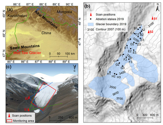
Figure 1.
(a) Location map of the Sawir Mountains and Muz Taw Glacier (red solid circle); (b) The glaciological mass-balance measuring network in 2019 (the background is from the ALOS (Advanced Land Observing Satellite) digital elevation model (DEM)), and the numbers denote elevations of the contours; (c) Spatially distributed scan positions (S1 and S2) and the extent of the terrestrial laser scanning (TLS) surveyed area (red rectangle) (the background is from Google Earth).
Muz Taw Glacier (47°04′ N, 85°34′ E) is a northeast-faced valley glacier that is situated on the northern side of the Sawir Mountains (Figure 1), with an area of 3.13 km2 and a length of 3.2 km in 2016 [33]. Glaciological investigations of Muz Taw Glacier were initiated in 2013, and subsequently, an observation and research station (Altai Observation and Research Station of Cryospheric Science and Sustainable Development, Chinese Academy of Sciences) was set up for the long-term measurements. According to the latest observations, the glacier area decreased continuously with a value of 10.51 km2 (45.72%) over the period 1977–2017, and the mean annual length change (front variation) reached up to 11.5 m a−1 from 1989 to 2017 [17]. The glacier is controlled by the prevailing westerlies in a continental climate setting, Jimunai Meteorological Station (984 m a.s.l., located about 46 km northeast of the glacier) showed that the average annual air temperature and precipitation were 4.3 °C and 212 mm, respectively, during the period 1961–2016. Both annual air temperature and precipitation presented an increasing trend with rates of 0.4 °C (10 a)−1 and 12 mm (10 a)−1, respectively. High air temperature mainly occurred from May to August, and air temperature was very low during winter. The annual distribution of precipitation was approximately homogeneous and precipitation in July was relatively high, and the winter precipitation accounted for 10–30% of the annual total (Figure 2).
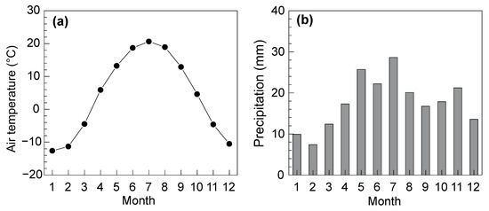
Figure 2.
Average air temperature (a) and precipitation (b) recorded by Jimunai Meteorological Station (located about 46 km northeast of Muz Taw Glacier at 984 m a.s.l.) from 1961 to 2016.
3. Data and Methods
3.1. TLS Surveys and Data Processing
As mentioned above, we utilized the Riegl VZ®-6000 TLS to acquire the glacier surface terrain. The TLS was produced by Riegl Laser Measurement Systems GmbH (Austria) in 2012 with a weight of 14.5 kg, and it was dust- and water-proof. The continuous operating voltage and air temperature range from 11 to 32 V and from −10 to 50 °C, respectively. The device can offer a maximum measurement range of 6 km for natural targets and high-speed data acquisition of 222,000 points per second. The angle measurement resolution is better than 0.0005° (1.8 arcsec), and laser divergence is 0.12 mrad (equivalent to an increase of 12 mm of beam diameter per 100 m distance). The scanning range ranges from 0 to 360° horizontally and from 60–120 °vertically (from zenith). The Riegl VZ®-6000 TLS is a well-established tool for measuring snowy and icy terrain even at long distances, since the device operates at the wavelengths in the near-infrared band (class 3B laser beams, 1064 nm), which enables high rates of reflection (>80%) [31]. Note that the volume-to-mass conversion factor is a fundamental issue for geodetic mass balance calculations (see Section 3.2); the TLS surveys are ideally carried out at the end of the ablation season to reduce the influence of fresh snow. Here, point clouds of the ablation area were acquired by the TLS surveys implemented on 13 September 2017, 4 September 2018, 13 September 2019, and 15 September 2020, and the ablation area was mainly covered with bare ice on the days of the TLS surveys (Figure 3). Specific measurements included three procedures.
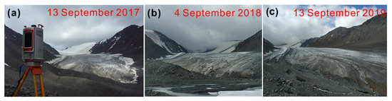
Figure 3.
TLS survey of the Muz Taw Glacier with the Riegl VZ®-6000 TLS in September 2017 (a), 2018 (b), and 2019 (c). The ablation area was mainly covered with bare ice.
(1) Placement of scan positions. According to [34] and our field experience, the placement of scan positions adhere to the following basic criteria: (a) scan positions must be placed in the stable terrain with broad perspectives and easily accessible; (b) scan positions should be distributed at different elevations around mountain glaciers, and the number of scan positions should be as small as possible to reduce error related to point cloud processing; (c) the distance between the scanner and the target should be within the scanning range, and the angle between the laser pulse and the target should be more than 10° to receive the echo of the laser pulse; (d) the overlap percentage of two neighboring scan positions should be more than 30% to guarantee the quality of data registration. Based on the aforementioned criteria, two scan positions were used for the TLS surveys, and their spatial distribution was presented in Figure 1c. We fixed each scan position on the stable bedrock by using a reinforced concrete structure; then, we combined and installed stainless steel measuring nails and protection boxes to build a standard GNSS-leveling (GNSS, Global Navigation Satellite System) point. Despite the visual angles of the two scan positions not being very ideal relative to the entire glacier surface, the TLS surveys completely covered the glacier tongue. In addition, we did not place scan positions at the right side of Figure 1c, since the region was covered with sand and gravel, and the terrain of the right side was unstable and steep, which will be detrimental to TLS surveys.
(2) Three-dimensional (3D) coordinate of the two scan positions. We used the real-time kinematic (RTK) GNSS of Trimble R10 to acquire coordinate, which was used for point cloud direct georeferencing (see data processing). Note that it is better to place some retro-reflective targets surveyed with the GNSS at much greater distances relative to scan positions, since the measuring accuracy will reduce with the increase of scanning range. However, this study mainly focused on the relative changes in glacier surface elevation between two consecutive scan campaigns, and the requirement of absolute accuracy was not very strong. Thus, we had not implemented this type of survey.
(3) Point cloud acquisition. We mounted the TLS on a sturdy tripod for each scan position after placement and 3D coordinate of scan positions. Considering that the environmental conditions around glaciers vary significantly, here, the input environmental parameters (air temperature, atmospheric pressure, relative humidity, and height above sea level) of the TLS surveys were provided by portable meteorological instruments and Trimble R10 GNSS. All of the four scan campaigns were carried out under an overcast sky to reduce the influence of atmospheric refraction (Figure 3) [31]. Note that the altitude drop and scanning range were relatively small, since this study only focused on the ablation area of the Muz Taw Glacier, which may result in unremarkable variations of atmospheric refraction. In addition, dry, fogless, and windless weather conditions were also considered to enhance measurement accuracy (see Section 3.5). After these steps, we configured the laser pulse repetition rate as 50 kHz to complete coarse scanning with vertical and horizontal angles range of 60–120° from zenith and 0~360°, respectively; then, the glacial regions of the coarse scanning images were selected to finish fine scanning with the laser pulse repetition rate of 30 kHz. Detailed surveying parameters are listed in Table 1.

Table 1.
Detailed survey parameters.
We processed point cloud by using RiSCAN PRO® v 1.81 software and the overall workflow used for data processing was given in Figure 4, which included direct georeferencing, data registration, compression, filtering, multi-temporal registration, and interpolation. The specific processes were as follows: (1) direct georeferencing, we used the 3D coordinates of the two scan positions to transform the point cloud data from the scanner’s own coordinate system into a global coordinate system [35]; (2) data registration, we used multi-station adjustment (MSA) to finish data registration of each scan position according to the iterative closest point (ICP) algorithms [36] and subsequently merged the two scans in one layer; (3) compression, an octree algorithm was used to compress the merged point cloud with a equal space of 0.5 m; (4) filtering, the terrain filter was used to filter out the noise and non-ground data; additionally, we used visual interpretation to check the data individually and deleted outliers [37]; and (5) multi-temporal registration, the attitude angles of each scan campaign are different as the orientation of each scan position is continually adjusted to complete data registration, which can lead to horizontal and vertical shifts between two consecutive scan campaigns and increase the error of TLS-derived DEM differencing. Thus, multi-temporal registration directly determined the accuracy of glacier surface elevation change [38,39]. Since the coarse scanning and fine scanning had the same attitude angles, for each scan campaign, we first removed the glacierized regions of the point clouds from coarse scanning, and then we set the processed point clouds of 2017 as the reference layer and used ICP algorithms to implement the alignment of scan campaigns in 2018, 2019, and 2020 based on the point clouds over stable non-glacier terrain. Hence, the point clouds of fine scanning between two consecutive scan campaigns can coincide well after these processes. Finally, interpolation of the processed point clouds from fine scanning created high-resolution DEMs (0.5 m) after multi-temporal registration.
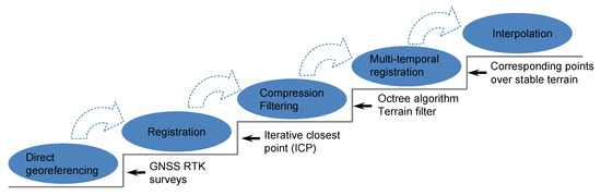
Figure 4.
Schematic illustration of the workflow used for point cloud processing. “GNSS” is the abbreviation of “Global Navigation Satellite System” and “RTK” is the abbreviation of “real-time kinematic”.
3.2. Geodetic Mass Balance
Geodetic mass balance is calculated as a multiplication between glacier volume change and volume-to-mass conversion factor [5]. Volume change ΔV over the TLS survey period between t0 and t1 can be determined as:
where r is the pixel size of TLS-derived DEM (0.5 m), is the glacier surface elevation change of the two consecutive DEMs at pixel k, and K denotes the number of total pixels covering the extent of the TLS surveyed area.
Glacier volume change ΔV is converted to geodetic mass balance (m water equivalent (w.e.)) using:
where is the mean glacier area of the two survey times, (1000 kg m−3) is the density of water, and is the volume-to-mass conversion factor for converting glacier volume change to mass balance. Here, we conservatively assumed that equaled the density of ice (900 kg m−3), since the monitoring area was mainly covered with bare ice on the days of the TLS surveys (Figure 3).
3.3. Glaciological Mass Balance
The glaciological mass balance of the Muz Taw Glacier had been implemented by measuring ablation stakes and snow pits; more than 20 stakes were drilled into the glacier using a steam drill and distributed in eight rows at different altitudes with roughly three stakes in every row (Figure 1b). The measurements include the stake vertical height above the glacier surface, superimposed ice thickness, and the density and thickness of each snow/firn layer at snow pits. The mass balance of each measured point can be calculated as the arithmetic sum of snow, glacier ice, and superimposed ice mass balance. Point values are extrapolated to glacier-wide mass balance using the contour-line or profile method [40,41].
3.4. Emergence Velocity
The geodetic surveys of glacier elevation change mainly include surface mass balance and vertical velocity [25]. The glaciological method measures the surface mass balance [42]. Therefore, conservation of mass at a point (ablation stake) on the surface of a glacier can be expressed as:
where is glacier surface elevation changes, is the glaciological mass balance, is density, and is ice flux. When Equation (3) is integrated over the entire glacier surface, becomes zero, and the glaciological mass balance equals the elevation change multiplied by the volume-to-mass conversion factor (i.e., geodetic mass balance). However, is not zero for a given point, and the vertical velocity () plays a confounding role [43].
As shown in Figure 5, vertical velocity refers to the upward or downward flow of ice relative to the glacier surface at a fixed coordinate, and it is called “emergence velocity” in the ablation area and “submergence velocity” in the accumulation area [25]. Emergence and submergence velocity result in dynamic thickening and thinning of a glacier, respectively [44]. Previous studies assume that emergence velocity depends on the kinematic boundary condition at the glacier surface [25,43] and can be calculated as:
where us and are the horizontal components of ice velocity at the glacier surface S [25,43]. We neglect the advection of the glacier surface topography induced by horizontal ice flux since short time intervals of the TLS surveys [45], which yields:
and for emergence velocity:
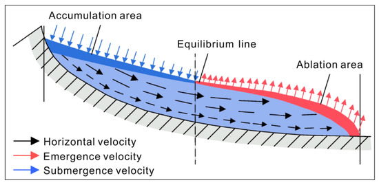
Figure 5.
Conceptual representation of the different velocity components, which was redrawn base on [25].
As described in Section 3.3, here, we used the point mass balance from glaciological measurements in 2018–2019 to estimate the emergence velocity for each individual ablation stake.
3.5. Uncertainty Estimates
The uncertainty in TLS-derived glacier surface elevation and mass changes depends on point cloud data acquisition and processing and volume-to-mass conversion [21]. Point cloud data acquisition corresponds to the stability of the two scan position and atmospheric conditions of the TLS surveys, and therefore, we fixed scan positions on stable rock surfaces to minimize the uncertainty. Additionally, point clouds of the glacier surface were acquired in dry, fogless, and windless weather conditions to reduce wind- and moisture-induced errors, since the wind will result in the vibration of the TLS instrument and moisture can absorb laser pulse. In addition, the systematic error of the device can also induce related uncertainty in data acquisition, but it varies greatly and cannot be quantified well, for instance, with the scanning distance to the target. So, we only discussed it in Section 5.1. For point cloud data acquisition processing error, the standard deviation of errors (σMSA) obtained from registering the point cloud can be used to evaluate multi-temporal registration quality [46], the resulting errors were in the range of 0.07–0.10 m and generally less than the error of TLS-derived glacier surface elevation (Table 2). We only discussed the results in Section 5.1. The octree algorithm built the topological relationship of scattered points, which can preserve terrain information as much as possible. The error related to DEM (with a resolution of 0.5 m) creation can be neglected because of the high average point density (1.90–5.21 points m−2, Table 1). For volume-to-mass conversion, the uncertainty of glacier ice density was assumed to be ± 17 kg m−3 according to [47].
Table 2.
Error (σMSA) of multi-station adjustment (MSA) and the number of points (n) used for multi-temporal registration of two consecutive TLS surveys, the uncertainty () of TLS-derived glacier surface elevation, and the corresponding uncertainty of geodetic () and glaciological () mass balance.
The standard deviation of the stable non-glacier terrain () was used to calculate the uncertainty of the TLS-derived glacier surface elevation () due to the lack of precise and well-distributed stable ground control points, but the spatial auto-correlation must be removed when we calculate the uncertainty of the glacier-wide elevation changes. Here, was quantified using the geostatistical analysis of [48] and expressed as:
where is the correlation area. We assume that because of the high point density (>1 point m−2) [49]. Uncertainty in geodetic mass balance () can be estimated using:
where is the mean value of the TLS-derived glacier elevation change. The calculated uncertainties are shown in Figure 6 and listed in Table 2.
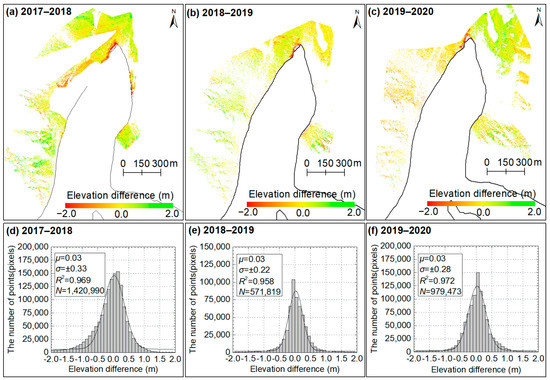
Figure 6.
Spatial distribution of surface elevation changes over stable non-glacier terrain (a–c) and corresponding frequency distributions of these changes (d–f). The median (μ), the standard deviation (σ), fitting coefficient (R2), and the number of pixels (N) are given.
Uncertainty in glaciological mass balance measurements at individual point locations originate from errors in stake readings, snow/firn probing, and the sinking of the stakes [42,50]. Following [51], the uncertainty of the glaciological method raised with the total number of sampling sites, corresponding error of ablation measured in ice, and firn was estimated to be about 0.14 w.e. a−1 and 0.27 w.e. a−1, respectively, and the error in accumulation measurements was 0.14 w.e. a−1, based on independent geodetic mass balance. Uncertainty in a given point can be calculated based on the law of error propagation [42]. Thus, errors of ablation measurements in ice () and firn () are evaluated using and , respectively, where and are the total number of ablation stakes and snow pits, respectively; errors in accumulation measurements () are determined based on , where is the number of snow pits. The total uncertainty in point annual mass balance () is calculated as:
Here, we mainly considered the measured errors in the ablation area and the calculated error was about 0.03 m w.e. a−1. Due to surface elevation change in the ablation area is the arithmetic sum of mass balance and the emergence velocities (), the uncertainty in emergence velocity can be calculated applying a reciprocal density conversion:
The resulting values are listed in Table 2 and discussed in Section 5.1.
4. Results
4.1. Glacier Surface Elevation and Geodetic Mass Changes
As shown in Figure 7, TLS-derived DEM differencing gives detailed spatial distributions of glacier surface elevation changes for the latest three mass-balance years. The ablation area of the Muz Taw Glacier showed clearly surface lowering and negative geodetic mass changes, with a value of −1.33 ± 0.13 m w.e a−1, −1.64 ± 0.09 m w.e a−1, and −1.01 ± 0.11 m w.e a−1, for the mass-balance years 2017–2018, 2018–2019, and 2019–2020, respectively. Spatial changing patterns were maintained as generally similar for all of the three investigated periods with the most negative surface lowering values ranged from −5.0 to −4.0 m a−1 near the glacier terminus and less pronounced thinning in the upper elevations. Measured glacier thinning was remarkably higher for the second period with 92.2% of the elevation change falling in the range −3.0 to −1.0 m, which was significantly more negative compared to the first and third mass-balance year (corresponding proportion was 79.6% and 60.2%, respectively). These temporal differences in observed glacier surface elevation and mass changes were consistent with summer (June–September) air temperature (11.4, 12.2, and 11.6 °C in summer 2018, 2019, and 2020, respectively) recorded by Jeminay (website: https://www.tianqi.com/, accessed on 1 March 2021), which showed a similar response to the observed climatic forcing compared to glaciers in other regions, demonstrating that glaciers in the Sawir Mountains were also sensitive to the warming climate.
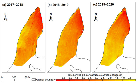
Figure 7.
Spatial distribution of TLS-derived glacier surface elevation changes at the ablation area of the Muz Taw Glacier for the latest three mass-balance years (a–c).
The altitudinal distribution of glacier elevation changes is a combination of glacier surface mass balance and dynamic processes (emergence/submergence velocities). The altitudinal profiles of glacier surface elevation changes were depicted in Figure 8 and showed thinning continuously decreased with increasing of altitude, which was a commonly changing behavior and agreed well with the knowledge of existing in situ measurements [8]. The altitudinal gradient was about 0.69 m (100 m)−1, 0.60 m (100 m)−1, and 0.95 m (100 m)−1, for the mass-balance years 2017–2018, 2018–2019, and 2019–2020, respectively, which showed a positive correlation (R2 = 0.93) with observed glacier mass balance, indicating that a higher altitudinal gradient of glacier surface elevation changes usually resulted in less mass loss. The gradient of altitudinal elevation changes was commonly steep at the low elevations and gentle in the upper-elevation parts (the turning point occurred at the altitude of 3210 m a.s.l. for all of the three periods). In addition, reduced surface lowering occurred at the glacier terminus, which was consistent with the glaciological mass balance versus elevation of most reference glaciers reported by [8].
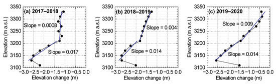
Figure 8.
Altitudinal (within 20 m elevation bands) profiles of glacier surface elevation changes at the ablation area of the Muz Taw Glacier for the latest three mass-balance years (a–c).
In order to identify aspect controls on the patterns of glacier surface elevation changes, we calculated the distribution by the aspect of the glacier area (in 2017) compared with the distribution of mean glacier surface elevation change. Results suggested that the mean glacier surface lowering on the eight aspects was in good agreement with the glacier mass loss of the three mass-balance years. The majority of the observed glacier area had aspects north through east, while more negative mean glacier surface changes were dominant for west, southwest, and south aspects with the exception of surface changes on the west aspect for the mass-balance year 2017–2018, confirming that aspect controlled glacier ablation, since it was possible to influence the glacier surface albedo and the TLS had potential for detailed investigation of the controls.
4.2. Surface Ablation and Emergence Velocity
In situ measurements of single-point mass balance were available by using the ablation stakes. Here, we selected the well-measured data in the mass balance year 2018–2019 to reflect glacier surface ablation and emergence velocity. Glaciological measurements revealed that significant surface ablation occurred at the row of C (−3.06 m w.e. a−1 at the ablation stake of C3), and the ablation at the row of “A” was relatively less negative, this changing pattern was consistent with TLS-derived glacier surface elevation changes (Figure 7 and Figure 8). Stakes in the row of “D-E” exhibited surface ablation between −2.50 w.e. a−1 and −1.50 w.e. a−1, less negative mass balance occurred at the uppermost stakes (H1 and H2), which was near with the TLS-derived glacier mass balance at the same elevation bands.
The calculated emergence velocities ranged from 0.11 to 0.86 m a−1, which slightly compensated for the surface ablation at the ablation area. The higher velocities happened at the ablation stakes of C1 and D1. The spatially distributed emergence velocity showed pronounced spatial variability, which decreased from the lower elevations to the upper glacierized regions (Figure 9). Spatial patterns in emergence velocities may be related to glacier surface slope; big slope or steep terrain was conducive to the downward migration of glacier mass and resulted in large horizontal velocities and small emergence velocities. Our comparisons between the emergence velocity and glacier surface slope at the ablation stakes exhibited an excellent correlation (Figure 10). Note that the spatial distribution of measured sites was insufficient, since a very small number of well-measured ablation stakes can be used, which may affect the correlation coefficient. So, the numerical results need more sites to validate it. In addition, the left side around the ablation stakes of C1 and D1 had thicker glacier ice with thickness in the range of 70–90 m according to ground penetrating radar measurements in 2013 [16]. To our knowledge, glacier thickness makes the most important contribution to ice velocity, which may result in higher velocities at the left regions [52]. The movement of tributary glaciers at the right side can slightly increase the flow of mass; thus, the ablation stake of E3 was characterized with higher velocity. However, those were only quite qualitative descriptions, and we needed more observations to validate the interpretations.
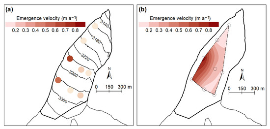
Figure 9.
Emergence velocity at each ablation stakes (a), interpolation of the spatially distributed emergence velocity by a kriging method (b) for the mass balance year 2018–2019.
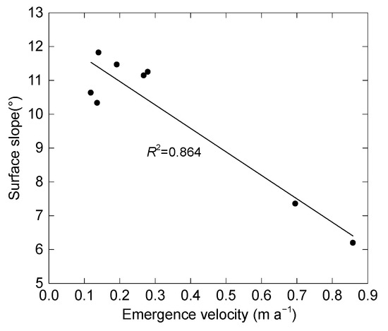
Figure 10.
Correlation between the emergence velocity and glacier surface slope at the ablation stakes.
5. Discussion
5.1. Accuracy of DEM Differencing and Geodetic Mass Balance
The fixed scan positions used in this study can enhance the stability of the TLS surveys, and we selected windless atmospheric conditions to reduce the vibration of the TLS device while scanning. Nevertheless, the TLS itself and glacier surface terrain can introduce some errors into the acquired point clouds. The systematic error of the TLS cannot quantify well, so the instrument manufacturers usually give simplified and constant values for the ranging accuracy and precision. For instance, the precision of Riegl VZ®-6000 TLS reported has been reported to be about 10 mm [31], which completely satisfies the measurement accuracy in glaciology. Terrain-induced errors refer to glacier surface characteristics or geometry and the incident angle between the target and the scanner (e.g., slope, aspect, and size of the targets) [53,54]. The applied TLS can achieve a scanning range of 6 km provided that the target size exceeds the laser beam footprint, perpendicular incident angle, and good atmospheric visibility [31]. For the purpose of this study, the established scan positions were situated at different elevations and directions relative to the glacier surface. Dry weather conditions and overcast sky were also selected to reduce the influence of atmospheric refraction [31]. Note that the laser beam footprint had reached up to the top elevations of the Muz Taw Glacier under these premises, but some voids existed at the accumulation area. This study chose the best-surveyed data at the ablation zone to guarantee the good quality of the TLS-derived DEMs.
Surface elevation changes over stable non-glacier terrain are used to evaluate the accuracy of DEM differencing, which exhibited normal distribution (Figure 6). Our statistics suggested that more than 80% and 90% of the total pixels with elevation changes fell in the confidence intervals of 2 × sigma and 3 × sigma, respectively, indicating that the accuracy of DEM differencing should be limited to the decimeter level. This may be related to fixed scan positions and the use of multi-temporal registration [38]. According to the point clouds over stable terrain, here, multi-temporal registration was used indispensably to correct the misalignment of two consecutive scan campaigns in the horizontal and vertical orientation via ICP algorithms due to the lack of in situ-measured ground control points [21,39].
On average, the uncertainty of TLS-derived geodetic mass balance was 0.11 m w.e. a−1 for the three investigated periods (Table 2). The accuracy of our results was close to the studies that used high-precision 3D laser scanning, such as Hintereisferner in Austria, with a mean error of 0.07 m w.e. a−1 [47], four very small glaciers in Switzerland, with a mean error of 0.13 m w.e. a−1 [21], and Echaurren Norte Glacier in Chilean Andes, with a mean error of 0.09 m w.e. a−1 [55]. However, the uncertainty estimated in our study was smaller than the similar studies that used coarse DEMs (e.g., [56,57,58]), confirming the high precision of the TLS surveys. Note that this study only focused on glacier mass balance in the ablation area, and uncertainties in estimated accumulation had not been considered, which probably improved the accuracy of geodetic mass balance [59].
5.2. Spatiotemporal Variability of Glacier Surface Elevation and Mass Changes
It is widely recognized that glacier mass balance is very sensitive to air temperature [60]. The aforementioned high air temperature in summer 2019 was one of the key factors for clearly negative surface elevation and mass changes in the second mass-balance year. Other factors, such as the topographical conditions, can also influence the spatial patterns in TLS-derived surface elevation changes. Our results suggested that altitudinal distributions of glacier surface slope and elevation changes exhibited opposite tendencies. The lower elevations presented steep terrain with slopes in the range of 16–18°, and clearly negative surface elevation changes were observed in those elevations (Figure 11a). A good correlation existed between the mean glacier surface slope and elevation changes over the three periods (Figure 11b). The steep terrain can increase the removal of large snow depositions and is detrimental to glacier accumulation. Note that the mean glacier surface slope at different elevation bands showed an increasing trend with continuous glacier ablation, which can contribute to accelerated glacier mass loss.
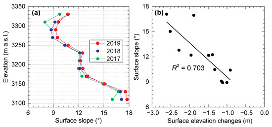
Figure 11.
(a) Altitudinal distributions of glacier surface slope in 2017, 2018, and 2019. (b) Correlation between the mean glacier surface slope and elevation changes over the three periods.
5.3. Influence of Emergence Velocity and Mass Balance on Surface Lowering
In order to estimate the influence of each component in the ablation zone quantitatively, the annual mass balance measured at the nine stakes in the mass-balance year 2018–2019 was compared to the emergence velocities (Figure 12). TLS-derived glacier surface elevation changes were dominated by surface ablation (the average value of stake height changes was −2.18 m), and the mean contribution of emergence velocity was only limited to be 0.33 ± 0.11 m, which slightly compensated the surface ablation with a mean percentage of 14.9%. The findings suggested that dynamic thickening had small contributions to glacier surface evolution at the ablation area, and glacier surface lowering was mainly controlled by mass balance; such findings could happen at other glaciers in the Sawir Mountains. With the continuous glacier mass loss (concomitant with ice thinning) and the reduction of accumulation area ratio, emergence velocity will gradually decrease, which in turn results in rapid glacier surface lowering [61]. For instance, a decline in emergence (−0.11 m) velocity had been observed at Qiyi Glacier in the Qilian Mountains from the periods 1975–1985 to 1986–2002 [62], and similar phenomena were also observed at Lirung Glacier in the Nepal Himalaya since 2000 [29].
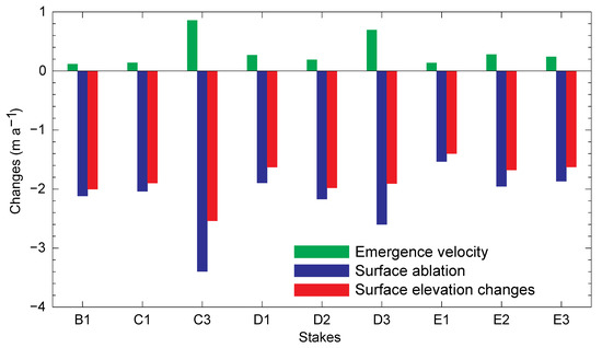
Figure 12.
Emergence velocity (green), in situ measured surface lowing due to ablation (blue) and TLS-derived glacier surface elevation changes at each ablation stake (red).
Here, we compared our results to previous similar studies to discuss the dynamic characteristics of different regions and types of glaciers and thus to investigate the possible mechanism of dynamic thickening. The estimated annual emergence velocity (0.33 m a−1) at the ablation area of the Muz Taw Glacier, which was close to the corresponding values of Urumqi Glacier No. 1 (0.20–0.30 m a−1) in the Tien Shan [63] and Qiyi Glacier (0.32–0.43 m a−1) in the Qilian Mountains [62], but it was significantly smaller than that of Parlung No. 4 Glacier (3.7 m a−1) in the southeastern Tibetan Plateau [64], the debris-covered ablation area of Khumbu Glacier (5.7 m a−1) in the Nepal Himalaya [29], the ablation area of Hintereisferner (5.0 m a−1) in the Central Alps [65], Kesselwandferner (0–5.0 m a−1) in the Ötztal Alps [27], and Mer de Glace (4.0 m a−1) in the French Alps [26]. Glaciers in northwestern China are dominated by cold type, and they are characterized by relatively smaller mass accumulation and ablation compared with temperate glaciers in the southeastern Tibetan Plateau and Alps [66]. Particularly for the Muz Taw Glacier, very less annual precipitation recorded by Jimunai Meteorological Station directly determined limited glacier accumulation, and our field observations also confirmed this. Thus, the weak dynamic thickening can potentially be attributed to poor mass accumulation.
5.4. Limitations and Further Work
Although the applied TLS can provide a scanning range of 6 km and the scanned area exceeded 4.0 km2 for the four years, our study only focused on a portion of the ablation area of (accounting for about 17.6% of the total glacier area) the Muz Taw Glacier, since some voids occurred at the upper elevations. This is mainly because of the limited scanning angle of the TLS. Auxiliary surveys from other techniques such as a cut-price unmanned aerial vehicle (UAV) can be required. Consequently, the combination of TLS and UAV had been done in many studies (e.g., [22,67,68]). A 30 m-high glacier monitoring tower had been placed at the fore of the glacier, which had a good visual angle relative to the entire glacier surface. Therefore, the TLS device can be mounted at the tower to increase the scanning range. For further work, we will integrate the TLS, UAV, and glacier monitoring tower to acquire the entire glacier surface terrain at the seasonal and monthly scales. In such a case, high-resolution and high-precision geodetic glacier mass balance can be yielded, which will bring insight into the mass balance processes and their mechanisms. Moreover, accurate quantification of the submergence/emergence velocities is important for geodetic mass balance estimates and simulation of the glacier dynamic process; therefore, we propose to strengthen the glaciological mass-balance measurements by using stakes and snow pits.
6. Conclusions
Glacier meltwater in the Sawir Mountains is an important freshwater resource for populations and hydro-economies in Jeminay and its surrounding counties; mass-balance measurements are fundamental to evaluate the impact of glacier changes on water resources. However, studies on detailed glacier mass changes are still vacant. This study presents high-precision evolution of annual surface elevation and geodetic mass changes in the ablation area of the Muz Taw Glacier (Sawir Mountains, China) over the latest three consecutive mass-balance years (2017–2020) based on multi-temporal terrestrial geodetic surveys. We mainly analyzed the spatiotemporal pattern of surface elevation and geodetic mass changes and the influences of emergence velocity on glacier surface lowering and discussed the possible mechanism of glacier dynamic thickening.
Our results revealed clearly surface lowering and negative geodetic mass changes, spatial changing patterns were maintained as generally similar for all of the three investigated periods with the most negative surface lowering (approximately −5.0 to −4.0 m a−1) around the glacier terminus and less pronounced thinning in the upper elevations, and the altitudinal increasing gradient was 0.69 m, 0.60 m, and 0.95 m per 100 m, for the mass-balance years 2017–2018, 2018–2019, and 2019–2020, respectively. The gradient of altitudinal elevation changes was commonly steep at the low elevations and gentle in the upper-elevation parts (the turning point occurred at the altitude of 3210 m a.s.l. for all of the three periods), and reduced surface lowering was observed at the glacier terminus. The majority of the more negative mean glacier surface changes were dominant for west, southwest, and south aspects, confirming that aspect had a major impact on glacier ablation. Calculated emergence velocities ranged from 0.11 to 0.86 m a−1 with pronounced spatial variability and higher velocities at the left and upper right sides, which were mainly controlled by surface slope, ice thickness, and the movement of tributary glaciers.
High air temperature in summer 2019 was one of the main factors for clearly negative surface elevation and mass changes in 2018–2019, and our foundlings suggested that glacier surface terrain can also influence surface elevation and mass changes. Emergence velocities made slight compensations to the surface ablation at the ablation area with a proportion of 14.9%, indicating that dynamic thickening had small contributions to the glacier surface evolution. The cold Muz Taw Glacier is located in a continental climate setting characterized by relatively smaller mass accumulation and ablation compared with temperature glaciers in the southeastern Tibetan Plateau and Alps, which can probably result in weak dynamic thickening. Our study only focused on a portion of the ablation area of the Muz Taw Glacier. In the follow-up work, we will integrate the TLS, UAV, and glacier monitoring tower to realize the whole glacier surface surveys at the seasonal and monthly scales, and submergence/emergence velocities should be carefully considered for geodetic mass balance estimates and simulation of glacier dynamic processes.
Author Contributions
Conceptualization, C.X. and Z.L.; methodology, C.X.; software, C.X.; validation, C.X., Z.L., and J.M.; formal analysis, C.X. and F.W.; investigation, Z.L.; data curation, C.X. and J.M; writing—original draft preparation, C.X.; writing—review and editing, C.X. and F.W.; visualization, C.X.; supervision, Z.L.; project administration and resources, C.X. All authors have read and agreed to the published version of the manuscript.
Funding
This research was funded by the National Natural Science Foundation of China (42001067), National Cryosphere Desert Data Center (20D03), the Strategic Priority Research Program of Chinese Academy of Sciences (XDA20020102), the Second Tibetan Plateau Scientific Expedition and Research (STEP) program (2019QZKK0201), and State Key Laboratory of Cryospheric Science (SKLCS-ZZ-2021).
Institutional Review Board Statement
Not applicable.
Informed Consent Statement
Not applicable.
Data Availability Statement
Data are available upon request by email to the corresponding author.
Acknowledgments
The authors sincerely thank the staff from Tien Shan Glaciological Station, Chinese Academy of Sciences, for providing the continuous TLS surveys.
Conflicts of Interest
The authors declare no conflict of interest.
References
- Hagg, W.J.; Braun, L.N.; Uvarov, V.N.; Makarevich, K.G. A comparison of three methods of mass-balance determination in the Tuyuksu glacier region, Tien Shan, Central Asia. J. Glaciol. 2004, 50, 505–510. [Google Scholar] [CrossRef]
- Kaser, G.; Cogley, J.G.; Dyurgerov, M.B.; Meier, M.F.; Ohmura, A. Mass balance of glaciers and ice caps: Consensus estimates for 1961–2004. Geophys. Res. Lett. 2006, 33, L19501. [Google Scholar] [CrossRef]
- Huss, M.; Hock, R. Global-scale hydrological response to future glacier mass loss. Nat. Clim. Chang. 2018, 8, 135–140. [Google Scholar] [CrossRef]
- Kääb, A.; Leinss, S.; Gilbert, A.; Bühler, Y.; Gascoin, S.; Evans, S.G.; Bartelt, P.; Berthier, E.; Brun, F.; Chao, W.; et al. Massive collapse of two glaciers in western Tibet in 2016 after surge-like instability. Nat. Geosci. 2018, 11, 114–120. [Google Scholar] [CrossRef]
- Zemp, M.; Huss, M.; Thibert, E.; Eckert, N.; McNabb, R.; Huber, J.; Barandun, M.; Machguth, H.; Nussbaumer, S.U.; Gärtner-Roer, I.; et al. Global glacier mass changes and their contributions to sea-level rise from 1961 to 2016. Nature 2019, 568, 382–386. [Google Scholar] [CrossRef]
- Yao, T.; Thompson, L.; Yang, W.; Yu, W.; Gao, Y.; Guo, X.; Yang, X.; Duan, K.; Zhao, H.; Xu, B.; et al. Different glacier status with atmospheric circulations in Tibetan Plateau and surroundings. Nat. Clim. Chang. 2012, 2, 663–667. [Google Scholar] [CrossRef]
- Hoelzle, M.; Azisov, E.; Barandun, M.; Huss, M.; Farinotti, D.; Gafurov, A.; Hagg, W.; Kenzhebaev, R.; Kronenberg, M.; Machguth, H.; et al. Reestablishing glacier monitoring in Kyrgyzstan and Uzbekistan, Central Asia. Geosci. Instrum. Method. Data Syst. 2017, 6, 397–418. [Google Scholar] [CrossRef]
- WGMS (World Glacier Monitoring Service). Global Glacier Change Bulletin No. 3 (2016–2017); ISC(WDS)/IUGG(IACS)/UNEP/UNESCO/WMO; Zemp, M., Gärtner-Roer, I., Nussbaumer, S.U., Bannwart, J., Rastner, P., Paul, F., Hoelzle, M., Eds.; World Glacier Monitoring Service: Zurich, Switzerland, 2020; pp. 1–274. [Google Scholar] [CrossRef]
- Brun, F.; Berthier, E.; Wagnon, P.; Kääb, A.; Treichler, D.A. spatially resolved estimate of High Mountain Asia glacier mass balances from 2000 to 2016. Nat. Geosci. 2017, 10, 668–673. [Google Scholar] [CrossRef]
- Gardelle, J.; Berthier, E.; Arnaud, Y.; Kääb, A. Region-wide glacier mass balances over the Pamir–Karakoram-Himalaya during 1999–2011. Cryosphere 2013, 7, 1263–1286. [Google Scholar] [CrossRef]
- Farinotti, D.; Longuevergne, L.; Moholdt, G.; Dustman, D.; Mölg, T.; Bolch, T. Substantial glacier mass loss in the Tien Shan over the past 50 years. Nat. Geosci. 2015, 8, 716–722. [Google Scholar] [CrossRef]
- Wei, J.; Liu, S.; Guo, W.; Xu, J.; Bao, W.; Shangguan, D. Changes in glacier volume in the north bank of the Bangong Co Basin from 1968 to 2007 based on historical topographic maps, SRTM, and ASTER stereo images. Arct. Antarct. Alp. Res. 2015, 47, 301–311. [Google Scholar] [CrossRef]
- Bolch, T.; Pieczonka, T.; Mukherjee, K.; Shea, J. Brief communication: Glaciers in the Hunza catchment (Karakoram) have been nearly in balance since the 1970s. Cryosphere 2017, 11, 531–539. [Google Scholar] [CrossRef]
- Yao, T.; Yu, W.; Wu, G.; Xu, B.; Yang, W.; Zhao, H.; Wang, W.; Li, S.; Wang, N.; Li, Z.; et al. Glacier anomalies and relevant disaster risks on the Tibetan Plateau and surroundings. Chin. Sci. Bull. 2019, 64, 2770–2782. [Google Scholar] [CrossRef]
- Panagiotopoulos, F.; Shahgedanova, M.; Hannachi, A.; Stephenson, D.B. Observed Trends and Teleconnections of the Siberian High: A Recently Declining Center of Action. J. Clim. 2005, 18, 1411–1422. [Google Scholar] [CrossRef]
- Huai, B.; Li, Z.; Wang, F.; Wang, W.; Wang, P.; Li, K. Glacier volume estimation from ice-thickness data, applied to the Muz Taw glacier, Sawir Mountains, China. Environ. Earth. Sci. 2015, 74, 1861–1870. [Google Scholar] [CrossRef]
- Wang, Y.; Zhao, J.; Li, Z.; Zhang, M. Glacier changes in the Sawuer Mountain during 1977–2017 and their response to climate change. J. Nat. Resour. 2019, 34, 802–814. [Google Scholar]
- Fischer, A. Comparison of direct and geodetic mass balances on a multi-annual time scale. Cryosphere 2011, 5, 107–124. [Google Scholar] [CrossRef]
- Schumann, G.J.; Bates, P.D. The need for a high-accuracy, open-access global DEM. Front. Earth Sci. 2018, 6, 225. [Google Scholar] [CrossRef]
- Immerzeel, W.W.; Kraaijenbrink, P.D.A.; Shea, J.M.; Shrestha, A.B.; Pellicciotti, F.; Bierkens, M.F.P.; Jong, S.M.D. High-resolution monitoring of Himalayan glacier dynamics using unmanned aerial vehicles. Remote Sens. Environ. 2014, 150, 93–103. [Google Scholar] [CrossRef]
- Fischer, M.; Huss, M.; Kummert, M.; Hoelzle, M. Application and validation of long-range terrestrial laser scanning to monitor the mass balance of very small glaciers in the Swiss Alps. Cryosphere 2016, 10, 1279–1295. [Google Scholar] [CrossRef]
- Fugazza, D.; Scaioni, M.; Corti, M.; D’Agata, C.; Azzoni, R.S.; Cernuschi, M.; Claudio, S.; Diolaiuti, G.A. Combination of UAV and terrestrial photogrammetry to assess rapid glacier evolution and map glacier hazards. Nat. Hazards Earth Syst. Sci. 2018, 18, 1055–1071. [Google Scholar] [CrossRef]
- Réveillet, M.; Vincent, C.; Six, D.; Rabatel, A.; Sanchez, O.; Piard, L.; Laarman, O. Spatio-temporal variability of surface mass balance in the accumulation zone of the Mer de Glace, French Alps, from multitemporal terrestrial LiDAR measurements. J. Glaciol. 2021, 67, 137–146. [Google Scholar] [CrossRef]
- Hooke, R.L. Principles of Glacier Mechanics, 3rd ed.; Cambridge University Press: Cambridge, UK, 2019; pp. 1–539. [Google Scholar]
- Cuffey, K.M.; Paterson, W.S.B. The Physics of Glaciers, 4th ed.; Academic Press: New York, NY, USA, 2010; pp. 1–704. [Google Scholar]
- Berthier, E.; Vincent, C. Relative contribution of surface mass balance and ice-flux changes to the accelerated thinning of Mer de Glace, French Alps, over 1979–2008. J. Glaciol. 2012, 58, 501–512. [Google Scholar] [CrossRef]
- Stocker-Waldhuber, M.; Fischer, A.; Helfricht, K.; Kuhn, M. Long-term records of glacier surface velocities in the Ötztal Alps (Austria). Earth Syst. Sci. Data 2019, 11, 705–715. [Google Scholar] [CrossRef]
- Deschamps-Berger, C.; Nuth, C.; Van Pelt, W.; Berthier, E.; Kohler, J.; Altena, B. Closing the mass budget of a tidewater glacier: The example of Kronebreen, Svalbard. J. Glaciol. 2019, 65, 136–148. [Google Scholar] [CrossRef]
- Nuimura, T.; Fujita, K.; Sakai, A. Downwasting of the debris-covered area of Lirung Glacier in Langtang Valley, Nepal Himalaya, from 1974 to 2010. Quat. Int. 2017, 455, 93–101. [Google Scholar] [CrossRef]
- Brun, F.; Wagnon, P.; Berthier, E.; Shea, J.M.; Immerzeel, W.W.; Kraaijenbrink, P.D.; Christian, V.; Camille, R.; Dibas, S.; Arnaud, Y. Ice cliff contribution to the tongue-wide ablation of Changri Nup Glacier, Nepal, central Himalaya. Cryosphere 2018, 12, 3439–3457. [Google Scholar] [CrossRef]
- RIEGL Laser Measurement Systems. 3D Terrestrial Laser Scanner Riegl VZ®-4000/Riegl VZ®-6000 General Description and Data Interfaces; RIEGL Laser Measurement Systems: Horn, Austria, 2014; pp. 1–466. [Google Scholar]
- Shi, Y. Concise China Glacier Inventory; Shanghai Science Popularization Press: Shanghai, China, 2005; pp. 1–490. [Google Scholar]
- Wang, F.; Yue, X.; Wang, L.; Li, H.; Du, Z.; Ming, J.; Li, Z. Applying artificial snowfall to reduce the melting of the Muz Taw Glacier, Sawir Mountains. Cryosphere 2020, 14, 2597–2606. [Google Scholar] [CrossRef]
- CH/Z 3017-2015. Technical Specifications for Three-Dimensional Laser Scanning; National Administration of Surveying, Mapping and Geo-Information of the People’s Republic of China: Beijing, China, 2015; pp. 1–17.
- Lichti, D.D.; Gordon, S.J.; Tipdecho, T. Error models and propagation in directly georeferenced terrestrial laser scanner networks. J. Surv. Eng. 2005, 131, 135–142. [Google Scholar] [CrossRef]
- Besl, P.; McKay, N. A method for registration of 3-D shapes. IEEE T. Pattern Anal. 1992, 14, 239–256. [Google Scholar] [CrossRef]
- Perroy, R.L.; Bookhagen, B.; Asner, G.P.; Chadwick, O.A. Comparison of gully erosion estimates using airborne and ground-based LiDAR on Santa Cruz Island, California. Geomorphology 2010, 118, 288–300. [Google Scholar] [CrossRef]
- López-Moreno, J.I.; Revuelto, J.; Rico, I.; Chueca-Cía, J.; Julián, A.; Serreta, A.; Serrano, E.; Vicente-Serrano, S.M.; Azorin Molina, C.; Alonso-González, E.; et al. Thinning of the Monte Perdido Glacier in the Spanish Pyrenees since 1981. Cryosphere 2016, 10, 681–694. [Google Scholar] [CrossRef]
- Fey, C.; Wichmann, V. Long-range terrestrial laser scanning for geomorphological change detection in alpine terrain–handling uncertainties. Earth Surf. Proc. Land. 2017, 42, 789–802. [Google Scholar] [CrossRef]
- Østrem, G.; Brugman, M. Glacier Mass-Balance Measurements: A Manual for Field and Office Work; NHRI Science Report; Arctic Institute of North America: Saskatoon, SK, Canada, 1991; pp. 1–224. [Google Scholar]
- Kaser, G.; Fountain, A.; Jansson, P. A Manual for Monitoring the Mass Balance of Mountain Glaciers, International Hydrological Programme (IHP-VI. Technical Documents in Hydrology 59); UNESCO: Paris, France, 2003; pp. 9–26. [Google Scholar]
- Zemp, M.; Thibert, E.; Huss, M.; Stumm, D.; Rolstad Denby, C.; Nuth, C.; Nussbaumer, S.U.; Moholdt, G.; Mercer, A.; Mayer, C.; et al. Reanalysing glacier mass balance measurement series. Cryosphere 2013, 7, 1227–1245. [Google Scholar] [CrossRef]
- Beedle, M.J.; Menounos, B.; Wheate, R. An evaluation of mass-balance methods applied to Castle Creek Glacier, British Columbia, Canada. J. Glaciol. 2014, 60, 262–276. [Google Scholar] [CrossRef]
- Banerjee, A. Brief communication: Thinning of debris-covered and debris-free glaciers in a warming climate. Cryosphere 2017, 11, 133–138. [Google Scholar] [CrossRef]
- Pettersson, R.; Jansson, P.; Huwald, H.; Blatter, H. Spatial pattern and stability of the cold surface layer of Storglaciären, Sweden. J. Glaciol. 2007, 53, 99–109. [Google Scholar] [CrossRef]
- Gabbud, C.; Micheletti, N.; Lane, S.N. Lidar measurement of surface melt for a temperate Alpine glacier at the seasonal and hourly scales. J. Glaciol. 2015, 61, 963–974. [Google Scholar] [CrossRef]
- Klug, C.; Bollmann, E.; Galos, S.P.; Nicholson, L.; Prinz, R.; Rieg, L.; Sailer, R.; Stötter, J.; Kaser, G. Geodetic reanalysis of annual glaciological mass balances (2001–2011) of Hintereisferner, Austria. Cryosphere 2018, 12, 833–849. [Google Scholar] [CrossRef]
- Rolstad, C.; Haug, T.; Denby, B. Spatially integrated geodetic glacier mass balance and its uncertainty based on geostatistical analysis: Application to the western Svartisen ice cap, Norway. J. Glaciol. 2009, 55, 666–680. [Google Scholar] [CrossRef]
- Joerg, P.C.; Morsdorf, F.; Zemp, M. Uncertainty assessment of multi-temporal airborne laser scanning data: A case study on an Alpine glacier. Remote Sens. Environ. 2012, 127, 118–129. [Google Scholar] [CrossRef]
- Huss, M.; Bauder, A.; Funk, M. Homogenization of long term mass balance time series. Ann. Glaciol. 2009, 50, 198–206. [Google Scholar] [CrossRef]
- Thibert, E.; Vincent, C.; Blanc, R.; Eckert, N. Glaciological and volumetric mass balance measurements: Error analysis over 51 years, Sarennes Glacier, French Alps. J. Glaciol. 2008, 54, 522–532. [Google Scholar] [CrossRef]
- Wang, P.; Li, Z.; Zhou, P.; Li, H.; Yu, G.; Xu, C.; Wang, L. Long-term change in ice velocity of Urumqi Glacier No.1, Tian Shan, China. Cold Reg. Sci. Technol. 2018, 145, 177–184. [Google Scholar] [CrossRef]
- Deems, J.S.; Painter, T.H.; Finnegan, D.C. Lidar measurement of snow depth: A review. J. Glaciol. 2013, 59, 467–479. [Google Scholar] [CrossRef]
- Hartzell, P.J.; Gadomski, P.J.; Glennie, C.L.; Finnegan, D.C.; Deems, J.S. Rigorous error propagation for terrestrial laser scanning with application to snow volume uncertainty. J. Glaciol. 2015, 61, 1147–1158. [Google Scholar] [CrossRef]
- Farías-Barahona, D.; Vivero, S.; Casassa, G.; Schaefer, M.; Burger, F.; Seehaus, T.; Iribarren-Anacona, P.; Braun, F.E.H.; Braun, H. Geodetic mass balances and area changes of Echaurren Norte Glacier (Central Andes, Chile) between 1955 and 2015. Remote Sens. 2019, 11, 260. [Google Scholar] [CrossRef]
- Barandun, M.; Huss, M.; Sold, L.; Farinotti, D.; Azisov, E.; Salzmann, N.; Usubaliev, R.; Merkushkin, A.; Hoelzle, M. Reanalysis of seasonal mass balance at Abramov glacier 1968–2014. J. Glaciol. 2015, 61, 1103–1117. [Google Scholar] [CrossRef]
- Thomson, L.I.; Zemp, M.; Copland, L.; Cogley, J.G.; Ecclestone, M.A. Comparison of geodetic and glaciological mass budgets for White Glacier, Axel Heiberg Island, Canada. J. Glaciol. 2017, 63, 55–66. [Google Scholar] [CrossRef]
- Wagnon, P.; Brun, F.; Khadka, A.; Berthier, E.; Shrestha, D.; Vincent, C.; Yves, A.; Delphine, S.; Vincent, C.; Arnaud, Y.; et al. Reanalysing the 2007–19 glaciological mass-balance series of Mera Glacier, Nepal, Central Himalaya, using geodetic mass balance. J. Glaciol. 2021, 67, 117–125. [Google Scholar] [CrossRef]
- Basantes-Serrano, R.; Rabatel, A.; Francou, B.; Vincent, C.; Maisincho, L.; Cáceres, B.; Galarraga, R.; Alvarez, D. Slight mass loss revealed by reanalyzing glacier mass balance observations on Glaciar Antisana 15 during the 1995–2012 period. J. Glaciol. 2016, 62, 124–136. [Google Scholar] [CrossRef]
- Mölg, T.; Maussion, F.; Yang, W.; Scherer, D. The footprint of Asian monsoon dynamics in the mass and energy balance of a Tibetan glacier. Cryosphere 2012, 6, 1445–1461. [Google Scholar] [CrossRef]
- Dehecq, A.; Gourmelen, N.; Gardner, A.S.; Brun, F.; Goldberg, D.; Nienow, P.W.; Etienne, B.; Christian, V.; Patrick, W.; Trouvé, E. Twenty-first century glacier slowdown driven by mass loss in High Mountain Asia. Nat. Geosci. 2019, 12, 22–27. [Google Scholar] [CrossRef]
- Sakai, A.; Fujita, K.; Duan, K.; Pu, J.; Nakawo, M.; Yao, T. Five decades of shrinkage of July 1st glacier, Qilian Shan, China. J. Glaciol. 2006, 52, 11–16. [Google Scholar] [CrossRef]
- Xu, C.; Li, Z.; Li, H.; Wang, F.; Zhou, P. Long-range terrestrial laser scanning measurements of annual and intra-annual mass balances for Urumqi Glacier No. 1, eastern Tien Shan, China. Cryosphere 2019, 13, 2361–2383. [Google Scholar] [CrossRef]
- Yang, W.; Zhao, C.; Westoby, M.; Yao, T.; Wang, Y.; Pellicciotti, F.; Zhou, J.; He, Z.; Miles, E. Seasonal Dynamics of a Temperate Tibetan Glacier Revealed by High-Resolution UAV Photogrammetry and In Situ Measurements. Remote Sens. 2020, 12, 2389. [Google Scholar] [CrossRef]
- Span, N.; Kuhn, M.H.; Schneider, H. 100 years of ice dynamics of Hintereisferner, Central Alps, Austria, 1894–1994. Ann. Glaciol. 1997, 24, 297–302. [Google Scholar] [CrossRef][Green Version]
- Xie, Z.; Liu, C. Introduction to Glaciology; Shanghai Popular Science Press: Shanghai, China, 2010; pp. 1–490. [Google Scholar]
- Müller, D.; Walter, T.R.; Schöpa, A.; Witt, T.; Steinke, B.; Gudmundsson, M.T.; Dürig, T. High-resolution digital elevation modeling from TLS and UAV campaign reveals structural complexity at the 2014/2015 Holuhraun eruption site, Iceland. Front. Earth Sci. 2017, 5, 59. [Google Scholar] [CrossRef]
- Son, S.W.; Kim, D.W.; Sung, W.G.; Yu, J.J. Integrating UAV and TLS approaches for environmental management: A case study of a waste stockpile area. Remote Sens. 2020, 12, 1615. [Google Scholar] [CrossRef]


Publisher’s Note: MDPI stays neutral with regard to jurisdictional claims in published maps and institutional affiliations. |
© 2021 by the authors. Licensee MDPI, Basel, Switzerland. This article is an open access article distributed under the terms and conditions of the Creative Commons Attribution (CC BY) license (https://creativecommons.org/licenses/by/4.0/).