Abstract
Attributed to the explosive adoption of large-span spatial structures and infrastructures as a critical damage-sensitive element, there is a pressing need to monitor cable vibration frequency to inspect the structural health. Neither existing acceleration sensor-utilized contact methods nor conventional computer vision-based photogrammetry methods have, to date, addressed the defects of lack in cost-effectiveness and compatibility with real-world situations. In this study, a state-of-the-art method based on modified convolutional neural network semantic image segmentation, which is compatible with extensively varying real-world backgrounds, is presented for cable vibration frequency remote and visual monitoring. Modifications of the underlying network framework lie in adopting simpler feature extractors and introducing class weights to loss function by pixel-wise weighting strategies. Nine convolutional neural networks were established and modified. Discrete images with varying real-world backgrounds were captured to train and validate network models. Continuous videos with different cable pixel-to-total pixel (C-T) ratios were captured to test the networks and derive vibration frequencies. Various metrics were leveraged to evaluate the effectiveness of network models. The optimal C-T ratio was also studied to provide guidelines for the parameter setting of monitoring systems in further research and practical application. Training and validation accuracies of nine networks were all reported higher than 90%. A network model with ResNet-50 as feature extractor and uniform prior weighting showed the most superior learning and generalization ability, of which the Precision reached 0.9973, F1 reached 0.9685, and intersection over union (IoU) reached 0.8226 when utilizing images with the optimal C-T ratio of 0.04 as testing set. Contrasted with that sampled by acceleration sensor, the first two order vibration frequencies derived by the most superior network from video with the optimal C-T ratio had merely ignorable absolute percentage errors of 0.41% and 0.36%, substantiating the effectiveness of the proposed method.
1. Introduction
Attributed to the expanded scale of civil and industrial constructions along with the explosive adoption of large-span spatial structures, prestressed steel structural systems, including tensioned membrane structure, cable-dome structure, string structure, and so forth, are being utilized for practical engineering at a visibly accelerating pace. In terms of infrastructure constructions, cable-stayed bridges and suspension bridges, especially long-span ones, are the main application scenarios of prestressed steel structures. Owing to the pressing transportation demand of geologically complicated and perilous regions, the inventory of cable-supported infrastructures features an inevitable increasing trend. As a critical component of prestressed steel constructions, cable is deemed to be crucial for in-service structural effectiveness. Apart from damages caused by wind, earthquake, and other natural disasters, the major culprits of cable deterioration are long-term accumulated damages posed by fatigue and corrosion. Characterized by small mass and damping along with high flexibility, cables are susceptible to vibration when subjecting to the excitation of external loads. It is non-ignorable that vibration is a life-cycle process for cables. Fatigue damages of cables along with damages of steel sleeves and bolts are long-standing durability issues mainly caused by normal vibration, while abnormal vibration often signifies the aggravation of fatigue cracking of sheaths, the water accumulation at the root, and the acceleration of cable corrosion, which would further weaken the structural integrity and even evolve into catastrophic failure. Consequently, cable is contended to be a critical kind of damage-sensitive element.
Existing cable tension measuring methods vary extensively [1]. Complementary devices are required by some of these methods to implement the measurement, including pressure sensor testing method and pressure gauge testing method. Though reliable accuracies can be yielded, the majority of such directly measured methods are stretched to limits in field practice in terms of portability issues of devices. Another huge challenge encountered by directly measured methods is that they are human-oriented state-of-the-practice methods that require substantial field labor. Periodic and manual inspection may become a large burden on the shoulders of stakeholders and asset owners. Indirectly measured methods are utilized to convert cable tension into other easily measured physical signals or metrics. Here, we name a few that have attracted both academia and industrial sectors. Correlation between the transmission velocity of vibration wave in designated medium and the cable tension is leveraged by vibration wave method. Static profile along with static analytical formula of cable segment is utilized to calculate cable tension by static profile method. Resistance strain gauge method derives cable tension from its strain. Correlation between force and displacement is leveraged by elongation method. Difference of stress is determined by electromagnetic sensor method leveraging the variation of magnetic flux of cable placed in electro-magnetic induction system [2]. Represented by anchoring removed method, some approaches even temporarily weaken structural integrity when executed and render operational service interruption. Abovementioned methods are qualitatively assessed with respect to device applicability, portability, cost-effectiveness, and precision, as contrasted in Table 1. Owing to inherent obstacles, the majority of the abovementioned methods are not applicable for conventional inspection and have yet to be promoted widely to structural health monitoring practice. Consequently, these methods are limited to theoretical researches to a large extent.

Table 1.
Assessments of eight existing cable tension measuring methods.
Flexural rigidity, boundary conditions, and sag or deflection of cable have implications on measuring precision. Nevertheless, for the majority of cables with considerable length and negligible rigidity, boundary conditions and flexural rigidity only have limited influence within a limited length near anchor ends [3]. In this context, vibration method dominates the practice for structural health monitoring due to its simplicity, device portability, and repeatability [4].
Vibration method indices for assessing cable tension in accordance with the correlation between vibration frequency and the former. Vibration frequency measuring is the primary and paramount means of vibration method, and cable tension could then be derived from inherent specification parameters and vibration frequencies [1,5]. For the sake of vibration frequency measuring, resorting to acceleration sensors-utilized conventional contact measuring method [6,7,8], albeit technologically mature and reliable in precision, simultaneous monitoring on discrete nodes is cost-consuming, because one separate sensor should be instrumented on each cable prior to measuring. Moreover, given the locational inaccessibility of some cables, sensor installation has considerable difficulties and potentially poses safety risks for practitioners. To this end, non-contact photogrammetry methods have been gathering increasing attention from both theoretical researches and structural health monitoring practice for the sake of reducing labor force investment and enhancing operational simplicity. Yet, existing non-contact photogrammetry methods for vibration frequency monitoring, largely to this date, are based on conventional machine vision to a large extent and cannot adapt to images with varying backgrounds. These methods, termed as task-specific methods, require a tremendous quantity of images with multiple backgrounds for robust results.
Methods and approaches in multiple fields are implemented to measure cable vibration frequency. Data-driven applications are still the exceptions and yet to be fully leveraged. The rise of learning-oriented frameworks shed lights on addressing the limitations of aforementioned methods. Deep learning approaches hold promise towards conducting cable vibration frequency monitoring remotely and in a non-contact manner. As a promising complementary or even an alternative of existing measuring methods, there is a pressing need to introduce deep learning solutions for cable vibration frequency remote visual monitoring.
This paper intends to present a novel deep learning-based non-contact visual method for cable vibration frequency remote monitoring in cable-supported structures. The present study is built on a thriving branch in the deep learning community, that is, semantic image segmentation utilizing a convolutional neural network (CNN). The novelty of the proposed method, which is more compatible with real-world scenarios, lies in introducing a state-of-the-art technology to tackle extensively varying backgrounds within cable images with equivalent or even more remarkable accuracies while largely retaining the superiority of conventional computer vision-based photogrammetry applications. Deployment efficiency could be improved owing to that models or algorithms are not required to be redeployed, and applicability of the method could be further enhanced. The present study aims to (1) modify and train CNN models for semantic image segmentation with desired learning and generalization ability to segment cables in images and (2) study the optimal cable pixel-to-total pixel (C-T) ratio within an image to provide guidelines for the parameter setting of monitoring system in further research and practical application. To fulfill above dual ends, as a typical data-driven learning-oriented approach, the following research questions should be solved: (1) How to capture imagery data and setup dataset since a high-quality diverse dataset is crucial for the success of a sophisticate CNN framework, and (2) how to eliminate the influence of a small C-T ratio on the model precision.
The remainder of this paper is organized as follows. Related works and current state of researches are reviewed in Section 2. Data acquisition and dataset setup process are elaborated in Section 3. The research methodology, rationale of deep learning solutions for cable vibration frequency visual monitoring, along with the establishing and modifying of CNN frameworks, are briefed in Section 4. Subsequently, Section 5 will proceed with the demonstration of the effectiveness of modified CNN frameworks, the selection of the CNN model with the most superior performance, cable vibration frequencies derived from time history and frequency domain diagrams, and the study of optimal C-T ratio. The implication of sampling frequency on monitoring precision will be discussed in Section 6. Additionally, this paper will be finalized with prominent contributions and a forward looking emphasized in Section 7.
2. Related Works
Broadly, structural health monitoring by resorting to deep learning solutions has been attempted in research communities that bear the potential of complementing even replacing human-oriented state-of-the-practice inspection. Deep learning applications can tackle structural health monitoring issues at both local and global levels. The former mainly involves the detection of damages, such as crack, spalling, delamination, rust, and bolt. Additionally, the latter includes displacement measurement, structural response analysis, modal identification, cable force monitoring, vibration serviceability, and so forth [9]. Particularly, pertinent to deep learning applications for cable health monitoring, many researches have dedicated to adopting CNN for cable numerical signal identification or assessment. Xin et al. [10] introduced a status-driven acoustic emission monitoring method by combing wavelet analysis and transfer deep learning. CNN was used to construct the relationship between scalograms of acoustic emission signals and cable status. Zhang et al. [11] considered that the behavior of cable can be implicitly represented by the measured cable force series. A data-driven method that detects cable damage from measured cable forces by recognizing biased patterns from the intact conditions was proposed. Pattern recognition problems for cable damage detection through time series classification in deep learning was solved by this method. Jeong et al. [12] presented an automated cable tension monitoring system using deep learning and wireless smart sensors. A fully automated peak-picking algorithm tailored to cable vibration was developed using a region-based CNN to apply the vibration-based tension estimation method to automated cable tension monitoring.
Prior researches also presented significant efforts towards non-contact photogrammetry of cable vibration frequency.
Pertinent to the application of conventional computer vision technology, many researches have concentrated a significant amount of attention and have been proven effective. Chen [13] presented a moving target image tracking method to estimate cable vibration frequency and tension. Followed by binarization, background differencing along with morphological image processing for moving target detection, Kalman filter implemented was utilized to track moving object. Pasted round white papers were treated as artificial markers when performing conventional computer vision methods. Conversely, without any predesignated markers, Ji et al. [14] proposed the optical flow method to calculate cable displacement in images and vibration frequency could be further derived. Analogously, without any artificial target, Chen et al. [15] developed a simple digital videogrammetric technique to perform ambient vibration measurement of stay cables and subsequently identify cable frequencies. Kim et al. [16] introduced a non-contact measurement method by using digital image processing. Digital image correlation, image transform function along with subpixel analysis were performed to estimate the cable vibration frequency and correct the tension in hanger cables. Later, Kim et al. [17,18] developed a vision-based monitoring system to estimate the tensile force of stay cables during traffic use. The image processing technique involved normalized cross correlation computation, subpixel estimation, and so forth. A remotely controlled pan-tilt drive was installed and the developed system was scaled up for the simultaneous monitoring of multiple cables. Feng et al. [5] presented a novel noncontact vision-based sensor for the determination of cable tension force and vibration frequency. Cable vibration frequency was monitored by the subpixel orientation code matching algorithm and Fourier transform. Xu et al. [19] developed a low-cost and non-contact vision-based system to measure deck deformation and cable vibration under pedestrian loading in the context of cable-stayed footbridge. Zhao et al. [20] proposed a vision-based approach to identify cable natural frequencies using handheld shooting of smartphone camera. Cable boundary was directly tracked in the captured video image sequence. Cable dynamic characteristics are identified according to its dynamic displacement responses in frequency domain.
It can be summarized that, in context of conventional computer vision applications, the notion of vibration frequency photogrammetry is equivalent to that of displacement photogrammetry. Relative displacement is simply required for vibration frequency monitoring. Tension and other dynamic responses could be further acquired by absolute displacement. Researches involved in structural displacement monitoring with applications of computer vision techniques were reviewed in [21]. Conventional computer vision applications for structural displacement and vibration frequency monitoring are lacking in adaptivity, albeit technologically mature, cost-effective, and portable models or algorithms still need to be redeployed when coping with varying application scenarios.
To the best of the authors’ knowledge, solutions endeavoring to measure cable vibration frequency by resorting to deep learning approaches have yet, to date, to be fully researched. We therefore contend that deep learning visual solutions, which are competent to tackle varying real-world backgrounds, to measure and monitor cable vibration frequency remotely for practical structural health monitoring purpose has yet to be solved.
3. Data Acquisition and Dataset Setup
3.1. Determination of Cable Category
Categories of cables applied to prestressed steel infrastructures include steel wire rope, steel strand, strip steel, parallel steel bundle, semi-parallel steel bundle, profile steel, and so forth. Steel strand is widely promoted in infrastructure engineering, especially cable-supported bridges, for its manifold and prominent merits. Apart from civil, industrial, and infrastructure constructions, cable is also a critical, even decisive, element in remote electric power delivery engineering, mining engineering, and aerial cableway, in which steel strand dominates the practical application. Consequently, as a representative kind of cable, steel strand was selected as the research object in the present study. As high precision with sub-pixel level has not been, to date, ensured by deep learning-based solutions, one single cable was treated as the research object, that is, there merely exists one single cable in one image or video, to ensure the effectiveness of the proposed framework to the maximum extent.
3.2. Implications of External Interferences
The first major concern is the rigid vibration of the image capture device. For measured cable, a relative still image capture device is the premise of vision-based photogrammetry. However, in field application, image capture devices are always subject to rigid vibration-induced motion, which is caused by external or natural factors such as wind and ground shake. Measuring precision might be then compromised to some extent. To eliminate the rigid vibration influence of image capture device, a postulated still target should be predesignated and be ensured in the field of view. The rigid vibration-induced frequencies could be then removed from the power spectrum of cable vibrations. Such a compensating mechanism was accepted by some studies [22,23,24].
Nevertheless, it was also substantiated by some researchers that merely limited influence could be exerted on frequencies of measured targets by the rigid vibration of image capture devices. To name a few, camera rigid vibration was not taken into consideration by Khuc et al. [25], but the first three order frequencies of structural natural frequencies identified from vision-based method and that obtained from acceleration data showed perfect matching; Chen [13] obtained an acceptable error of 2%, ignoring the rigid vibration of the camera; a maximum error of 5.6% was observed by Feng et al. [5] without calculating and removing rigid vibration-induced frequencies. Consequently, given the limited influence of the rigid vibration along with the superiority vibration damping capacity of advanced camera support devices, the rigid vibration of image capture devices was also ignored in the present study.
Another external interference that must be taken into consideration is sampling frequency of the image capture device. According to Nyquist–Shannon sampling theorem [26], a signal should be sampled with a frequency larger than twice the maximum frequency contained in the signal, that is:
to ensure that information in the original signal can be completely restored and theoretically reconstructed from the sampled signal.
In the present study, first order frequencies of cables in cable-supported infrastructures and large-span spatial structures were empirically estimated to be 0–10 Hz, and the second order frequencies to be 10–20 Hz. Consequently, the restoring of second order frequencies is possibly hindered by the default shooting frame rate of 30 Hz of the image capture device. To this end, 60 Hz was set to be the shooting frame rate in the present research, also termed as sampling frequency, to study whether second order frequencies can be monitored. The implication of sampling frequency on the measuring precision will be later discussed in Section 6.
3.3. Data Acquisition
Numerical data was collected and imagery data was captured in Shaoxing, China. It was indicated by pre-testing that vibration frequencies of photographed cables with large length and small rigidity are within the monitorable range.
In the present study, numerical data indices for acceleration information sampled by acceleration sensors, which was treated as contrasted data for error estimation since vibration frequencies could be derived from the acceleration information. Imagery data involves two parts, that is, discrete cable images and continuous videos of vibrating cable. The former was utilized for the training and validation of CNN models, and the latter for the testing and the deriving of vibration frequencies.
3.3.1. Acquisition of Discrete Cable Images
Deep learning application to a real-world monitoring scenario requires diverse sampling of real-world context due to the variation of viewing angle, illumination, distance, and background in cable visual appearance. Owing to the regularity geometrical shape of steel strands, viewing angle has no implication on the appearance in the plane perpendicular to the cable. Consequently, varying illuminations and distances, along with multiple backgrounds were taken into consideration when capturing images in this situation. Excluded multiple viewing angles were also considered when capturing images in other photograph planes. Original size of captured discrete images was 4608 × 2308 pixels.
These discrete images were captured to train and validate CNN models to properly segment cables from backgrounds. Partial discrete images with varying viewing illuminations and distances along with multiple viewing angles and backgrounds are shown in Figure 1.
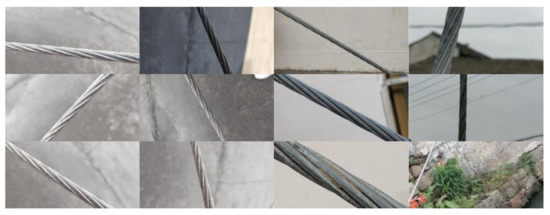
Figure 1.
Discrete images for the training and validation of convolutional neural network (CNN) models.
3.3.2. Acquisition of Continuous Videos of Vibrating Cable
Studying the optimal C-T ratio within an image necessitates the determination of the maximum and minimum value. 0.12 was determined as the maximum value and 0.01 as the minimum value, since the former is the maximum to ensure that the vibrating cable is kept in the frames and the latter is the minimum to ensure that features of cable appearance can be clearly captured. Three discontinuous values were inserted in the interval of the maximum and minimum, that is, 0.02, 0.04, and 0.08, and so that C-T ratio was divided into five levels. The optimal C-T ratio that can ensure the reliability of measuring precision would be selected within these five values.
To capture continuous videos of vibrating cable with different C-T ratios, a tripod was utilized to fix the video capture device at an adequate height and position to ensure that the still cable is in the center of frames, so that the photographed range of cable vibration can be maximized. The long axis of the video capture device was set to be parallel to the cable vibration plane. The sampling frequency was set to 60 Hz. Afterwards, the distance between tripod and cable along with the focal length was adjusted to ensure that C-T ratio is 0.12, 0.08, 0.04, 0.02, and 0.01, respectively. Finally, artificial external excitation was exerted on the cable and videos were captured simultaneously. The capture duration is 30–60 s.
Five continuous videos were captured, and the original frame size was 1920 × 1080 pixels. Continuous videos were utilized to derive vibration frequencies and study the optimal C-T ratio. Discrete images captured from five videos were utilized as testing set to assess the generalization ability of CNN models. The fixed focal length was set to 4.1 mm. Distances between video capture device and the cable, and digital zoom multiples are summarized in Table 2. Screenshots from five videos with different C-T ratios are shown in Figure 2.
Table 2.
Video photography related parameters.
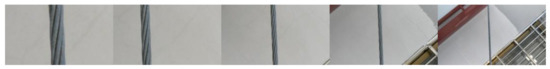
Figure 2.
Screenshots of continuous videos with different cable pixel-to-total pixel (C-T) ratios (left to right, 0.12, 0.08, 0.04, 0.02, and 0.01, respectively)
3.3.3. Acquisition of Numerical Data
An acceleration sensor was stationed on the cable in the plane perpendicular to vibration, so that Z axis of the sensor was parallel to the vibration plane. Sampling frequency was set to 200 Hz. Simultaneous with the photography of continuous videos, three sets of time history signals were sampled by the acceleration sensor, as plotted in Figure 3. Derived first and second order frequencies are listed in Table 3. It is noteworthy that three set of frequencies are numerically close to each other. Consequently, their averaged values, instead of original data, were adopted for error evaluation and the optimal C-T ratio determination.
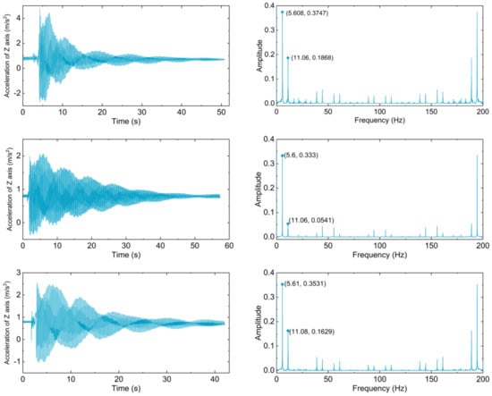
Figure 3.
Time history diagrams and frequency domain diagrams derived from acceleration samplings of Z axis by acceleration sensor.
Table 3.
Frequencies sampled by the acceleration sensor and their average values.
3.4. Image and Video Preprocessing, Data Augmentation and Dataset Annotation
In order to keep in line with the size of testing images, discrete images with varying real-world situations were resized to 1920 × 1080 pixels. Few blurred images with too much noise were deleted. Motivated by improving the generalization ability and the capacity of resisting disturbance of semantic segmentation models, and eliminate the influence of potential overfitting, data augmentation was implemented for the rest images. Detailed approaches for data augmentation include rotation, horizontal shift, vertical shift, shear, zoom, and horizontal flip. A total of 600 discrete images were collected after data augmentation. After image shuffling, training and validation sets were randomly balanced with a ratio of five to one, that is, training set accounted for 500 images and validation set for 100.
Dataset annotation was implemented to annotate the cable within images. Cables were annotated as “1” in binary and visualized to be dark blue while backgrounds as “0” and to be light blue, as shown in Figure 4.
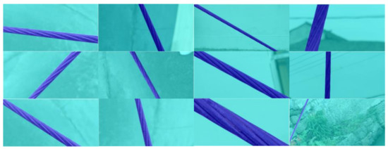
Figure 4.
Annotated discrete images in training and validation set.
Owing to that training and validation set were divided randomly after shuffling, overall C-T ratio distributions of training, and validation images can be reflected by that of the validation set. As demonstrated in Figure 5, images with C-T ratios smaller than 0.25 account for 99%, and the ones smaller than 0.125 account for 45%. It can be consequently concluded that cables are small targets contrasted with backgrounds.
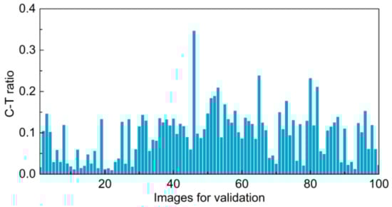
Figure 5.
C-T ratios of images in validation set.
For continuous videos with five different C-T ratios, 50 separate screenshots were captured from each of them to set up a testing set containing 250 images. The testing set was utilized to assess the generalization ability of segmenting cables from disturbances of CNN models.
4. Methodology
4.1. Deep Learning Solutions for Cable Vibration Frequency Visual Monitoring
Before going into the details about the establishing and modifying of CNN frameworks proposed in the present study, varying deep learning strategies for cable vibration frequency monitoring are briefed in this section, as this is beneficial to the understanding of the superiority of the presented framework.
Deep learning-based visual solutions applied to cable vibration frequency monitoring mainly involve two strategies, that is, recognizing-matching strategy and end-to-end multi-target tracking strategy.
4.1.1. Recognizing-matching Strategy
The key insight behind recognizing–matching strategy is first to recognize the target object within each image or frame, and then a matching algorithm is leveraged to match the target in adjacent frames, so that the motion of targets can be tracked. In this strategy, CNN frameworks are regarded as target recognition algorithms, which can efficiently extract the features of monitored targets contrasted with conventional computer vision algorithms. Additionally, conventional computer vision solutions for image processing are still adopted as the matching algorithms. Consequently, CNN target recognition framework plays a decisive role with respect to the effectiveness of the global framework.
Relative displacement can be obtained by CNN target recognition frameworks, including two-dimensional (2D) target detection frameworks and image segmentation frameworks. Absolute displacement could be further acquired after camera calibration. Typical 2D target detection frameworks are capable to figure out the positions of the objects with bounding boxes, mainly involve You Only Look Once (YOLO) [27], Single Shot MultiBox Detector (SSD) [28], Regions with CNN features (R-CNN) [29], and their variants. Image segmentation mainly refers to semantic segmentation and instance segmentation, the former can be formulated as a pixel-wise classification problem with semantic labels and the latter as partitioning of individual objects [30]. Outstanding frameworks include SegNet [31] and Mask R-CNN [32]. CNN models tailored for image classification, such as AlexNet [33], VGGNet [34], GoogLeNet [35], MobileNet [36], etc., are usually regarded as elementary structures of 2D target detection and image segmentation frameworks.
Advanced three-dimensional (3D) target recognition frameworks can directly take advantage of depth perception information from radar or point cloud, and the absolute displacement or real size of objects could be directly measured. Representative models include YOLO-6D [37], SSD-6D [38], and so forth.
4.1.2. End-to-end Multi-target Tracking Strategy
End-to-end multi-target tracking strategy mainly consists of two parts, feature extractor and similarity extractor. Instead of merely introducing deep learning models in the first target recognition module, interframe similarity parameter is introduced in feature extracting process by this strategy. An end-to-end framework is built up by feature extracting (recognition) in conjunction with interframe tracking (matching). Typical frameworks for this strategy include Siamese FC [39], SiamMask [40], and Siamese RPN++ [41].
Abovementioned two strategies along with convention computer vision solution are summarized and contrasted in Table 4. Though researches have been attracted to end-to-end tracking strategy, and recognizing–matching strategy with advanced 3D target recognition frameworks is becoming a mainstream research topic, they are not that viable in practice owing to their hardware-demanding, time-consuming, and computational complexities. Given that cables do not always appear as regular rectangles in images, the presented cable segmentation problem could not be addressed by 2D target detection frameworks. Owing to that proposed framework is a single-target recognition model, so instance segmentation frameworks and matching algorithms are not necessary. Consequently, recognizing–matching strategy with semantic segmentation framework (without matching algorithm) is adopted by the present study.
Table 4.
Recognizing–matching strategy and end-to-end multi-target tracking strategy.
To summarize, the internal processes of the presented framework involve (1) recognizing the contour boundary of cable and segmenting the cable from backgrounds, (2) extracting the centroid of the segmented area, and (3) deriving time history and frequency domain diagram after Fourier transform, vibration frequencies could then be acquired.
4.2. Establishing and Modifying of CNN Models
In the present study, in accordance with recognizing–matching strategy with semantic segmentation framework, nine CNN frameworks were established for training and comparative study, among which the one with the most superior performance would be selected for cable vibration frequency monitoring.
An effective underlying framework is deemed to be crucial for the success of subsequent works. There are two structures for semantic segmentation in deep neural networks, that is, encoder–decoder structure represented by U-Net [42] and SegNet [31], and spatial pyramid pooling module represented by DeepLab series. DeepLabv3+ [43] is an effectiveness-proven framework that takes advantage of both these two structures. A simple yet effective decoder module was designed by DeepLabv3+ to extend DeepLabv3 [44] which is treated as an encoder module. Segmentation results, especially along object boundary contours, can be refined. Besides, the depth-wise separable convolution was applied to DeepLabv3+. Above multiple improvements result in a faster and more robust encoder–decoder network. Consequently, DeepLabv3+ was selected as the underlying framework in the present study.
Prominent demerits of the underlying DeepLabv3+ framework lie in its huge computational expenses and compromised segmenting precision of small targets, albeit superior in generalization ability and robustness.
For the first demerit, to be specific, cable segmenting task is substantially a pixel-wise classification task with respect to cable versus disturbances. Xception [45] is treated as the sophisticate and task-specific feature extractor in DeepLabv3+. It is nonignorable that in the context of binary pixel-wise classification, Xception is structurally complicated and computationally complex. Additionally, the excessive increment of parameters and weights will also lead to overfitting. Consequently, another two simpler CNN models were utilized as feature extractors to provide alternatives to Xception. The underlying principle for the selection of simpler feature extractors is that the precision will be increased with a similar increment of the increasing training and testing duration time so that whether the trade-off—reducing duration time in exchange of the decreasing precision—is worthwhile can be estimated. It was expected that time elapsed during training, validation, and testing and segmenting precision could be balanced, and the time can be shortened while largely retaining the precision. ResNet-18 and ResNet-50 [46] were selected as alternative feature extractors since they have fewer parameters and simple yet effective residual blocks. For the sake of accelerating the convergence of networks and eliminating the influence of potential overfitting, which could possibly lead to inferior generalization ability, it is noteworthy that instead of being retrained globally, three feature extractors were adopted in the context of transfer learning. Lower-order layers of CNN extract features that are not specific to a particular task, whereas features extracted by high-level layers are specific to the task [47,48,49], so that low-order features could be transferred to professional cable dataset by transfer learning. Most parameters which were trained using original ImageNet dataset [50] were retained and frozen, and only the ones with the last few layers were retrained. Important properties of ResNet-18, ResNet-50, and Xception are contrasted in Table 5. The schematic of relative scale, duration time of training, validation and testing, and precision of three CNNs is shown in Figure 6.
Table 5.
Important properties of ResNet-18, ResNet-50, and Xception.
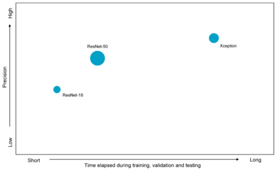
Figure 6.
Schematic of relative scale, duration time of training, validation and testing, and precision of three feature extractors.
For the second demerit, to be specific, as stated in Section 3.4, cables are small targets contrasted with backgrounds. It was indicated by the pre-training of original DeepLabv3+ that global accuracies of training and validation sets were higher than 90%. For pixel-wise class accuracies, that of background pixels were higher than 90%, yet that of cable pixels were lower than 20%. Data imbalance showed significant influence on segmenting precision. Consequently, class weights were introduced by weighting strategies to address the obstacle of data imbalance.
Weighted cross entropy was adopted in the present study as the loss function. Weight parameter β in weighted cross entropy is leveraged to increase or decrease the loss value of positive sample. The calculation of class weight W is the prerequisite of the determination of β. Three weighting strategies, inverse frequency weighting, median frequency weighting, along with uniform prior weighting were introduced to calculate W, respectively. In inverse frequency weighting, W is defined as:
where, refers to the number of pixels of a specific class, and denotes the total number of pixels. In median frequency weighting, W is defined as:
where, denotes the number of images that include instances of a specific class. In uniform prior weighting, W is defined as:
where, refers to the number of classes.
In the present study, β was defined as:
where, refers to the class weight of cable, and denotes that of backgrounds. was set to ensure that the influence of classification results of cable pixels on loss value was extended.
Inverse frequency weighting, median frequency weighting, along with uniform prior weighting were leveraged to pass class weights to pixel classification layer of DeepLabv3+ framework. It is indicated by calculation that for training and validation images, total number of pixels is 1.0368 × 10⁹, among which cable pixels account for 5.9812 × 10⁷ and background pixels for 9.7699 × 10⁸. Original cable pixel-to-background pixel ratio of training and validation images and that after weighting by three strategies are listed in Table 6. Evidently, the weight of cable pixel was significantly increased by weighting strategies.
Table 6.
Original cable pixel to background pixel ratio of training and validation images and that after weighting.
To summarize, the first modification of the underlying framework is adopting alternative simpler feature extractors to eliminate the influence of possible overfitting and simplify computational complexity. Additionally, the second modification is introducing class weights to loss function in pixel classification layer by three weighting strategies to eliminate the influence of data imbalance. Nine combinations were acquired by combining three feature extractors and three weighting strategies. Additionally, nine modified CNN frameworks were acquired in accordance with nine such combinations, which were named as Net-I–Net-IX, respectively. Modifications of nine CNN frameworks are listed in Table 7. Nine modified CNN frameworks are visualized in Figure 7, Figure 8, Figure 9 and Figure 10, among which the underlying framework is plotted in Figure 7, and three feature extractors are visualized in Figure 8, Figure 9 and Figure 10.
Table 7.
Modifications of nine CNN frameworks.
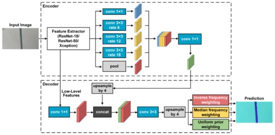
Figure 7.
Detailed structure of the underlying framework of modified CNN frameworks.
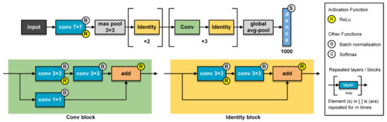
Figure 8.
Detailed structure of the ResNet-18 feature extractor (adopted in Net-I, Net-II, and Net-III).
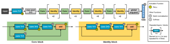
Figure 9.
Detailed structure of the ResNet-50 feature extractor (adopted in Net-IV, Net-V, and Net-VI).
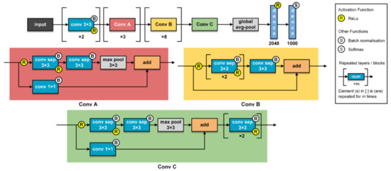
Figure 10.
Detailed structure of the Xception feature extractor (adopted in Net-VII, Net-VIII, and Net-IX).
4.3. Training Hyperparameter Optimizing and Assigning
Deep learning tasks usually encounter huge challenges when tuning training hyperparameters. Three important hyperparameters, initial learning rate, batch size, and epoch were optimized, which have possible significant implications on training and validation. Search ranges of three hyperparameters were determined by preliminary training in advance. Accounting for the feasibility, several discrete values were specified within their search ranges, as listed in Table 8. The rest major training hyperparameters and their adequate fixed options are summarized in Table 9.
Table 8.
Search sets of training hyperparameters to be optimized.
Table 9.
Fixed training hyperparameters and their options.
5. Results
All programs in the present study were performed with MatlabR2020a and Python 3.8, on a desktop computer equipped with 3.4 GHz Intel i5-7500 CPU, 8GB RAM, x-64 based processor and NVIDIA GeForce GT1030 GPU.
5.1. Optimal Training Hyperparameters
Training hyperparameters were optimized by minimizing segmentation error of the validation set, that is, optimal training hyperparameters were selected based on validation accuracy, as illustrated in Table 10.
Table 10.
Optimal training hyperparameters for nine CNN models.
5.2. Metrics and Evaluations of Training and Validation Set
5.2.1. Training and Validation Accuracies
Training with the optimal hyperparameters, training and validation accuracies reached by nine CNN models are listed in Table 11.
Table 11.
Training and validation accuracies of nine CNN models.
It is indicated in Table 11 that all the training and validation accuracies reached by nine CNN models are extremely close to each other, and hover around 95%. The Top-3 training and validation accuracies were reached by Net-I, Net-II, and Net-IV. Merely similar influences were exerted on training and validation accuracies by three different feature extractors and weighting strategies. Networks with computationally complex feature extractors, such as ResNet-50 and Xception, are not significantly superior, even inferior, to that with simpler feature extractors in terms of training and validation accuracies, by which our considerations when modifying networks are substantiated.
It is illustrated by accuracy and loss curves of training and validation that nine CNN models converged with similar rates. Accuracy curves rose and loss curves dropped rapidly, indicating that our diverse dataset was set reasonably. In terms of time elapsed during training, training for three epochs lasted 23–25 minutes for ResNet-18-adopted Net-I, Net-II, and Net-III, 63–68 minutes for ResNet-50-adopted Net-IV, Net-V, and Net-VI, and 187–189 minutes for Xception-adopted Net-VII, Net-VIII, and Net-IX.
In summary, nine CNN models performed undoubted learning ability during training and validation. Apart from the time elapsed during training and validation, the rest metrics have merely ignorable differences.
5.2.2. Aggregate Dataset Metrics and Class Metrics for Validation Set
Owing to the ignorable difference of training and validation accuracies, several aggregate dataset metrics and class metrics were leveraged to evaluate the validation set against ground truth.
For cable and background pixels, Precision and Recall are defined as:
where, TP, FP, TN, and FN denote the number of pixels of true positive, false positive, true negative, and false negative, respectively. Detailed connotations of TP, FP, TN, and FN are listed in Table 12. For our binary pixel-wise classification of cable versus backgrounds, the former is regarded as the positive class and the latter as the negative class, as visualized in Figure 11.
Table 12.
Confusion matrix for binary classification.
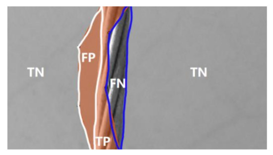
Figure 11.
Schematic diagram of confusion matrix metrics for cable versus backgrounds pixel-wise classification.
Precision and Recall are class metrics. Class metrics were averaged to set aggregate dataset metric, and further comprehensively and globally evaluated the effectiveness of CNN models. For Precision, corresponding aggregate dataset metric is termed as mean Precision (Pm), and calculated as:
Aggregate dataset metric corresponding to Recall were not set owing to that Recall is not commonly used in practice. Nevertheless, Precision and Recall values are usually integrally considered in the form of harmonic mean with a distance error tolerance, which is termed as , to decide whether predicted class of pixels has a match with the ground truth. is defined as:
As a class metric, an aggregate dataset metric was set in analogy to , termed as mean BF-score (). Mean BF-score is short for boundary contour matching score that measures how close the predicted boundary of the cable matches the ground truth boundary. Consequently, it is worth noting that only concentrate its attention on boundary pixels since this is visually more identical to human cognition. can be calculated as:
Note that the prediction and ground truth of merely cable boundary pixels are taken into consideration of the calculation of TP, FN, and FP here.
Besides, intersection over union (IoU) is commonly adopted for segmentation evaluation, which is defined as:
Additionally, two aggregate dataset metrics were set in analogy to IoU, that is, mean IoU () and weighted IoU (), which are calculated as:
Heretofore, four aggregate dataset metrics, include , , , and , and three class metrics, include Precision, , and IoU were leveraged to evaluate the validation set against ground truth, as illustrated in Table 13 and Table 14.
Table 13.
Evaluations of validation set with aggregate dataset metrics.
Table 14.
Evaluations of validation set with class metrics of cable class.
In aggregate dataset metrics, networks reached Top-3 s are Net-II, Net-V, and Net-VI, that reached Top-3 s are Net-II, Net-VI, and Net-VIII, and that reached Top-3 s and s are Net-I, Net-II, and Net-VI.
In class metrics for cable class, networks reached Top-3 Precisions are Net-II, Net-V, and Net-VI, that reached Top-3 s are Net-V, Net-VI, and Net-VII, and that reached Top-3 IoUs are Net-I, Net-II, and Net-VI.
To summarize, Net-II and Net-VI had the most superior learning ability when evaluated with training and validation set.
5.3. Metrics and Evaluations of Testing Set
Generalization ability was evaluated and contrasted with the testing set comprising 250 discrete images captured from five continuous videos with different C-T ratios. Evaluations are composed of two parts: (1) Macroscopically, class metrics of cable class were calculated for segmented results against ground truths which were annotated in advance and (2) microscopically, for the same testing image, segmentation results were visualized as heat maps, the matching of cable boundary contours and the internal recognition were observed.
For computational simplicity and feasibility, testing images were resized to 480 × 270 pixels for Net-I–Net-VI and 640 × 360 pixels for Net-VII–Net-IX. Testing images were read at 25 FPS.
For testing images with the C-T ratio of 0.12, 0.08, 0.04, 0.02, 0.01, class metrics of cable class are illustrated in Table 15, Table 16, Table 17, Table 18 and Table 19. Visualized segmentation results are plotted in Figure 12, Figure 13, Figure 14, Figure 15 and Figure 16, respectively. The sequence of horizonal and vertical pixels in testing images were represented by the numbers on the X-axis and Y-axis. The confidence scores of each pixel being the cable pixel were mapped to the corresponding colors which were arranged in the color gradation on the right. Clearer boundary contours and fewer blue areas (recognized as backgrounds) refer to the better segmentation.
Table 15.
Class metrics of cable class of testing images with the C-T ratio of 0.12.
Table 16.
Class metrics of cable class of testing images with the C-T ratio of 0.08.
Table 17.
Class metrics of cable class of testing images with the C-T ratio of 0.04.
Table 18.
Class metrics of cable class of testing images with the C-T ratio of 0.02.
Table 19.
Class metrics of cable class of testing images with the C-T ratio of 0.01.
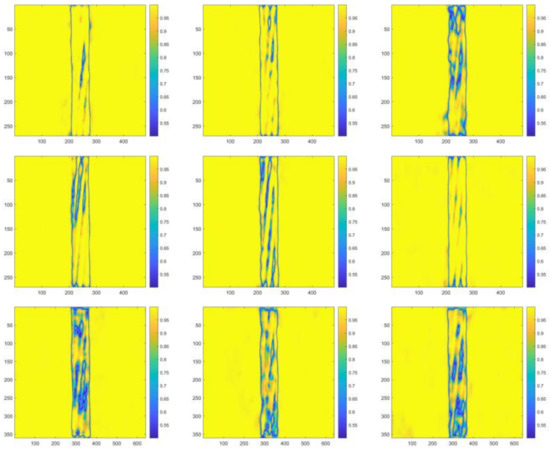
Figure 12.
Visualized segmentation results in the heat map form of the same representative testing image with the C-T ratio of 0.12 (left to right, top to bottom, Net-I–Net-IX, respectively, hereinafter).
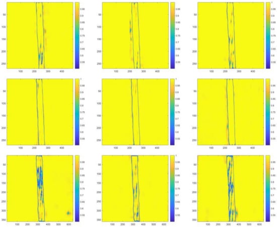
Figure 13.
Visualized segmentation results in the heat map form of the same representative testing image with the C-T ratio of 0.08.
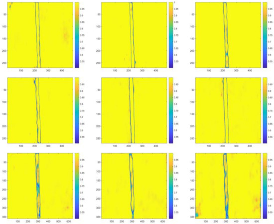
Figure 14.
Visualized segmentation results in the heat map form of the same representative testing image with the C-T ratio of 0.04.
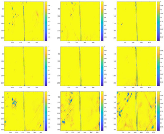
Figure 15.
Visualized segmentation results in the heat map form of the same representative testing image with the C-T ratio of 0.02.
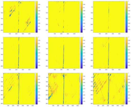
Figure 16.
Visualized segmentation results in the heat map form of the same representative testing image with the C-T ratio of 0.01.
It is evidently illustrated by above tables and figures that for testing images with the C-T ratio of 0.12, Net-I, Net-II, and Net-VI performed better; for that of 0.08, 0.04, 0.02, as well as 0.01, Net-V and Net-VI performed better. Alternatively, it can also be observed that for testing images with the C-T ratio of 0.12, more cable internal areas were prone to be recognized as background, and these areas are regularly distributed, which are the stranding areas of steel wires in steel strands. A conclusion can be preliminarily drawn that 0.12 might not be the optimal C-T ratio since the relatively high false recognition rate. Conversely, more disturbances in background were incorrectly recognized as cable areas when C-T ratio is small. Besides, testing with images with all the five different C-T ratios, without any exception, Xception-adopted Net-VII, Net-VIII, and Net-IX are observed to be the most ineffective networks. A prominent overfitting problem emerged with Xception-adopted networks. Satisfactory agreements are observed between testing results and the consideration stated in Section 4.2 when modifying CNN frameworks.
To sum up, Net-VI is the best-performing CNN model and has the best generalization ability.
5.4. Cable Vibration Frequency Deriving and the Determination of the Optimal C-T Ratio
Above arguments indicate that all the nine modified CNN models have learned the features of cables and successfully segmented cables from backgrounds, presenting outstanding learning and generalization ability. Demonstrated by comprehensive comparisons, Net-VI showed undeniable the most superior performance and was consequently selected as the representative achievement of the present study. Net-VI was named as CableNet for further discussion.
CableNet was utilized to semantically segment five continuous videos frame-by-frame. The abscissa of centroid of the area segmented as the cable was extracted for each frame, and the time history diagram was derived. Frequency domain diagram was further acquired with Fourier transform. When deriving frequency domain diagram from time history diagram, owing to that the vibrating cable was beyond photographed view in few frames, the abscissa of cable area centroid of these frames could not be obtained. These very few abscissa values were replaced by random numbers.
Derived time history and frequency domain diagrams are plotted in Figure 17. Derived first and second order frequencies were contrasted with that sampled by acceleration sensor to study the optimal C-T ratio, as listed in Table 20.
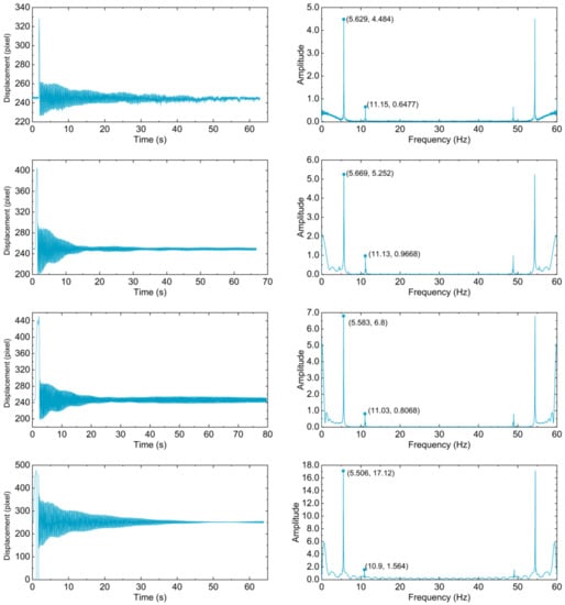
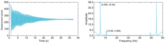
Figure 17.
Time history diagrams and frequency domain diagrams of the vibrating cable in five continuous videos (top to bottom, C-T ratio is 0.01, 0.02, 0.04, 0.08, 0.12, respectively).
Table 20.
Comparison of cable vibration frequencies sampled by acceleration sensor and that derived from videos.
As illustrated in Table 20, contrasted with that sampled by acceleration sensor, absolute percentage errors of first and second order frequencies are all less than 2%, which substantiate the effectiveness of proposed method. When C-T ratio is set to be 0.04, both the errors of first two order frequencies are less than 0.5%, shown undoubted the optimal results. Bigger or smaller C-T ratios bring larger percentage errors. To figure out the reason, the cable covers a larger area when C-T ratio is set bigger, detailed internal appearance of cable may be misrecognized as disturbances. As C-T ratio getting smaller, linear background objects may be misrecognized as cables, and even boundary contours of the cable could not be clearly segmented. Above arguments can be substantiated by the testing results visualized in Figure 12, Figure 13, Figure 14, Figure 15 and Figure 16.
Consequently, 0.04 is determined as the optimal C-T ratio to provide guidelines for the parameter setting of the monitoring system in future researches and practical applications.
5.5. Comparative Study
CableNet was compared with existing acceleration sensor-utilized method and methods proposed by [13,16,20,51], as summarized in Table 21. Markedly, cost-effectiveness and portability of device were enhanced by CableNet along with methods in [13,16,20,51] without any degradation of measuring precision. Additionally, only CableNet is compatible with extensively varying real-world backgrounds, address the limitations of conventional computer vision methods. Prominent merit and effectiveness of presented semantic image segmentation and CNN-based monitoring method are highlighted by comparative studies.
Table 21.
Comparative study of CableNet, existing acceleration sensor-leveraged method, and method proposed by references.
To summarize, according to aforementioned consecutive processes of CNN framework establishing and modifying, CNN model training, validation, and testing, along with the study of the optimal C-T ratio, working flow, and research process of the present study, are visualized in Figure 18.
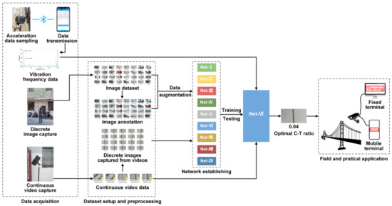
Figure 18.
Working flow and research process of the present study.
6. Discussion
As stated in Section 3.2, to ensure that information in the original signal can be completely restored, 60 Hz was set to be the sampling frequency when capturing continuous videos, which was proven effective. Yet, the computation expenses are relative huge, and the 60Hz sampling frequency is hardware-demanding. Consequently, sampling frequency of five 60 Hz videos were decreased to 30 Hz. The cable in five videos with 30 Hz sampling frequency were segmented by CableNet. Frequency domain diagrams and first two order frequencies were rederived, as illustrated in Figure 19 and Table 22.
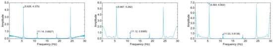
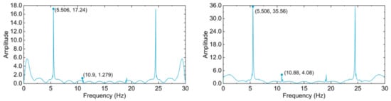
Figure 19.
Frequency domain diagrams of the vibrating cable in five videos with 30 Hz sampling frequency (top to bottom, left to right, C-T ratio is 0.01, 0.02, 0.04, 0.08, 0.12, respectively).
Table 22.
First two order frequencies derived from videos with sampling frequency of 30 Hz and 60 Hz.
It is indicated by above table and diagrams that nearly identical first two order frequencies can be derived from the videos with two different sampling frequencies. It can be consequently concluded that the sampling frequency of 30 Hz is also applicable for cable vibration frequency monitoring.
7. Conclusions
In the present study, a novel deep learning method based on modified CNN semantic image segmentation was presented for cable vibration frequency remote and visual monitoring. As a typical data-driven, learning-oriented approach, the key insight behind this method lies in feeding diverse dataset to CNN models which are enabled to extract implicit features and generalizing such features to newly fed data for segmentation.
DeepLabv3+ was selected as the underlying CNN framework. The underlying framework was modified in terms of (1) adopting alternative simpler feature extractors, ResNet-18, ResNet-50, and Xception, to eliminate the influence of possible overfitting and simplify computational complexity and (2) introducing class weights to loss function in pixel classification layer by three weighting strategies, inverse frequency weighting, median frequency weighting and uniform prior weighting, to eliminate the influence of data imbalance. Nine CNN frameworks were established and modified. CNN models were trained and validated with training and validation set containing 600 discrete images. 250 discrete screenshots captured from five continuous videos were utilized to test CNN models. High training and validation accuracies along with various aggregate dataset metrics and class metrics indicated their undoubted learning and generalization ability. Net-VI was selected as the representative achievement of the present study and was further named as CableNet since its most superior performance. CableNet is a semantic image segmentation model that adopted DeepLabv3+ as the underlying framework, ResNet-50 as feature extractor and uniform prior weighting as weighting strategy.
CableNet was utilized to semantically segment five continuous videos of vibrating cable with different C-T ratios frame-by-frame to measure vibration frequencies. Satisfactory agreements were observed between derived vibration frequencies and that sampled by acceleration sensor. Absolute percentage errors were all less than 2%, substantiating the effectiveness of the proposed method. The minimum error was observed when C-T ratio is 0.04. Consequently, 0.04 was determined as the optimal C-T ratio. The present study also found that apart from 60 Hz, the sampling frequency of 30 Hz is also applicable for cable vibration frequency monitoring.
The contributions of this research lie in:
- As a multi-disciplinary research, this study introduced a state-of-the-art method to conventional structural health monitoring community and widened the application scenarios of intelligent learning-oriented method. The semantic segmentation framework was algorithmically modified and adjusted for cable vibration frequency monitoring;
- CableNet can effectively overcome the defects of the applicability of varying backgrounds and cost-effectiveness that have not been, to date, addressed by conventional computer vision solutions, acceleration sensor-utilized methods, as well as prior researches;
- The presented CableNet could likely be scaled up for other similar cable vibration frequency monitoring tasks by transfer learning, so that application scenarios could be widened and the algorithm or model deployment efficiency could be enhanced regardless of the scenario complexity.
The prominent merit of the presented method lies in that it is compatible with extensively varying real-world backgrounds and can realize real-time cable vibration frequency monitoring remotely and in a non-contact manner just by industrial-grade video capture devices. However, the proposed learning-oriented method does not intend to be a cure-all. Although a high-quality cable dataset was collected, a more diverse dataset is required to cover more scenarios and monitor more kinds of cables. This is also the shortcoming of all data-driven methods. However, this trade-off—a diverse dataset with incredible care and exhausted efforts in exchange for a more precise monitoring system with broader applicability—is deemed to be worthwhile and economical.
Future works could be built on the restoration of blurred images caused by cables vibrating at higher frequencies, so that to further facilitate the building of a more sophisticate and robust cable and structural health visual monitoring system stepping forward.
Author Contributions
Conceptualization, H.-C.X. and S.-J.J.; methodology, H.Y. and H.-C.X.; software, H.-C.X.; validation, formal analysis, investigation, resources, data curation, H.Y. and H.-C.X.; writing—original draft preparation, H.Y. and H.-C.X.; writing—review and editing, H.Y., H.-C.X., and S.-J.J.; visualization, H.Y. and F.-D.Y.; supervision, S.-J.J.; project administration, H.Y. and F.-D.Y. All authors have read and agreed to the published version of the manuscript.
Funding
This research received no external funding.
Data Availability Statement
The data presented in this study are available on request from the corresponding author. The data are not publicly available as they involve the subsequent application of patent, software copyright and the publication of project deliverables.
Conflicts of Interest
The authors declare no conflict of interest.
References
- Guo, M.Y.; Chen, Z.H.; Liu, H.B.; Wu, X.F.; Li, X.B. Research progress of cable force test technology and cable flexural rigidity. Spat. Struct. 2016, 22, 34–43. (In Chinese) [Google Scholar] [CrossRef]
- Sumitro, S.; Jarosevic, A.; Wang, M.L. Elasto-magnetic sensor utilization on steel cable stress measurement. In Proceedings of the 1st Fib Congress, Concrete Structures in the 21th Century, Osaka, Japan, 13–19 October 2002; pp. 13–19. [Google Scholar]
- Irvine, H.M. Cable Structures; The MIT Press: Cambridge, MA, USA, 1981; pp. 20–60. [Google Scholar]
- Fang, Z.; Wang, J.-Q. Practical formula for cable tension estimation by vibration method. J. Bridge Eng. 2012, 17, 161–164. [Google Scholar] [CrossRef]
- Feng, D.M.; Scarangello, T.; Feng, M.Q.; Ye, Q. Cable tension force estimate using novel noncontact vision-based sensor. Measurement 2017, 99, 44–52. [Google Scholar] [CrossRef]
- Missoffe, A.; Chassagne, L.; Topçu, S.; Ruaux, P.; Cagneau, B.; Alayli, Y. New simple optical sensor: From nanometer resolution to centimeter displacement range. Sens. Actuator A Phys. 2012, 176, 46–52. [Google Scholar] [CrossRef]
- Gao, Z.; Zhang, D. Design, analysis and fabrication of a multidimensional acceleration sensor based on fully decoupled compliant parallel mechanism. Sens. Actuator A Phys. 2010, 163, 418–427. [Google Scholar] [CrossRef]
- Park, K.-T.; Kim, S.-H.; Park, H.-S.; Lee, K.-W. The determination of bridge displacement using measured acceleration. Eng. Struct. 2005, 27, 371–378. [Google Scholar] [CrossRef]
- Dong, C.-Z.; Catbas, F.N. A review of computer vision-based structural health monitoring at local and global levels. Struct. Health Monit. 2021, 20, 692–743. [Google Scholar] [CrossRef]
- Xin, H.; Cheng, L.; Diender, R.; Veljkovic, M. Fracture acoustic emission signals identification of stay cables in bridge engineering application using deep transfer learning and wavelet analysis. Adv. Bridge Eng. 2020, 1, 1–16. [Google Scholar] [CrossRef]
- Zhang, Z.; Yan, J.; Li, L.; Pan, H.; Dong, C. Condition assessment of stay cables through enhanced time series classification using a deep learning approach. In Proceedings of the 1st International Project Competition for Structural health monitoring (IPC-SHM), Harbin, China, 15 June–30 September 2020. [Google Scholar]
- Jeong, S.; Kim, H.; Lee, J.; Sim, S.-H. Automated wireless monitoring system for cable tension forces using deep learning. Struct. Health Monit. 2020. [Google Scholar] [CrossRef]
- Chen, Z.C. Cable Force Identification Based on Non-Contact Photogrammetry System. Master’s Thesis, Hunan University, Changsha, Hunan, China, 2015. (In Chinese). [Google Scholar]
- Ji, Y.F.; Chang, C.C. Nontarget image-based technique for small cable vibration measurement. J. Bridge Eng. 2008, 13, 34–42. [Google Scholar] [CrossRef]
- Chen, C.-C.; Tseng, H.-Z.; Wu, W.-H.; Chen, C.-H. Modal frequency identification of stay cables with ambient vibration measurements based on nontarget image processing techniques. Adv. Struct. Eng. 2012, 15, 929–942. [Google Scholar] [CrossRef]
- Kim, S.-W.; Kim, N.-S. Dynamic characteristics of suspension bridge hanger cables using digital image processing. NDT E Int. 2013, 59, 25–33. [Google Scholar] [CrossRef]
- Kim, S.-W.; Jeon, B.-G.; Kim, N.-S.; Park, J.-C. Vision-based monitoring system for evaluating cable tensile forces on a cable-stayed bridge. Struct. Health Monit. 2013, 12, 440–456. [Google Scholar] [CrossRef]
- Kim, S.-W.; Kim, N.-S.; Jeon, B.-G.; Park, J.-C. Vision-based monitoring system for estimating cable tensile forces of cable-stayed bridge. In Proceedings of the 7th International Conference on Bridge Maintenance, Safety and Management (IABMAS), Shanghai, China, 7–11 July 2014; pp. 970–977. [Google Scholar]
- Xu, Y.; Brownjohn, J.; Kong, D. A non-contact vision-based system for multipoint displacement monitoring in a cable-stayed footbridge. Struct. Control. Health Monit. 2018, 25, 1–23. [Google Scholar] [CrossRef]
- Zhao, X.; Ri, K.; Wang, N. Experimental Verification for Cable Force Estimation Using Handheld Shooting of Smartphones. J. Sens. 2017, 2017, 1–13. [Google Scholar] [CrossRef]
- Ye, X.W.; Dong, C.Z. Review of computer vision-based structural displacement monitoring. China J. Highw. Transp. 2019, 32, 21–39. (In Chinese) [Google Scholar] [CrossRef]
- Xu, Y.; Brownjohn, J.M.W. Review of machine-vision based methodologies for displacement measurement in civil structures. J. Civ. Struct. Health Monit. 2018, 8, 91–110. [Google Scholar] [CrossRef]
- Feng, D.M.; Feng, M.Q. Computer vision for SHM of civil infrastructure: From dynamic response measurement to damage detection–A review. Eng. Struct. 2018, 156, 105–117. [Google Scholar] [CrossRef]
- Lydon, D.; Lydon, M.; Taylor, S.; Del Rincon, J.M.; Hester, D.; Brownjohn, J. Development and field testing of a vision-based displacement system using a low cost wireless action camera. Mech. Syst. Signal Proc. 2019, 121, 343–358. [Google Scholar] [CrossRef]
- Khuc, T.; Catbas, F.N. Completely contactless structural health monitoring of real-life structures using cameras and computer vision. Struct. Control. Health Monit. 2017, 24, 1–17. [Google Scholar] [CrossRef]
- Shannon, C.E. Communication in the presence of noise. Proc. I.R.E. 1949, 37, 10–21. [Google Scholar] [CrossRef]
- Redmon, J.; Divvala, S.; Girshick, R.; Farhadi, A. You only look once: Unified, real-time object detection. In Proceedings of the IEEE Conference on Computer Vision and Pattern Recognition (CVPR), Las Vegas, NV, USA, 27–30 June 2016; pp. 779–788. [Google Scholar] [CrossRef]
- Liu, W.; Anguelov, D.; Erhan, D.; Szegedy, C.; Reed, S.; Fu, C.-Y.; Berg, A.C. SSD: Single shot multibox detector. In Proceedings of the 14th European Conference on Computer Vision (ECCV), Amsterdam, The Netherlands, 11–14 October 2016; pp. 21–37. [Google Scholar] [CrossRef]
- Girshick, R.; Donahue, J.; Darrell, T.; Malik, J. Rich feature hierarchies for accurate object detection and semantic segmentation. In Proceedings of the IEEE Conference on Computer Vision and Pattern Recognition (CVPR), Columbus, OH, USA, 23–28 June 2014; pp. 580–587. [Google Scholar] [CrossRef]
- Minaee, S.; Boykov, Y.; Porikli, F.; Plaza, A.; Kehtarnavaz, N.; Terzopoulos, D. Image segmentation using deep learning: A survey. arXiv 2020, arXiv:2001.05566. [Google Scholar]
- Badrinarayanan, V.; Kendall, A.; Cipolla, R. SegNet: A deep convolutional encoder-decoder architecture for image segmentation. IEEE Trans. Pattern Anal. Mach. Intell. 2017, 39, 2481–2495. [Google Scholar] [CrossRef]
- He, K.M.; Gkioxari, G.; Dollar, P.; Girshick, R. Mask R-CNN. IEEE Trans. Pattern Anal. Mach. Intell. 2020, 42, 386–397. [Google Scholar] [CrossRef] [PubMed]
- Krizhevsky, A.; Sutskever, I.; Hinton, G.E. ImageNet classification with deep convolutional neural networks. Commun. ACM 2017, 60, 84–90. [Google Scholar] [CrossRef]
- Simonyan, K.; Zisserman, A. Very deep convolutional networks for large-scale image recognition. In Proceedings of the International Conference on Learning Representations (ICLR), San Diego, CA, USA, 7–9 May 2015. [Google Scholar]
- Szegedy, C.; Liu, W.; Jia, Y.; Sermanet, P.; Reed, S.; Anguelov, D.; Erhan, D.; Vanhoucke, V.; Rabinovich, A. Going deeper with convolutions. In Proceedings of the IEEE Conference on Computer Vision and Pattern Recognition (CVPR), Boston, MA, USA, 8–10 June 2015; pp. 1–9. [Google Scholar] [CrossRef]
- Howard, A.G.; Zhu, M.L.; Chen, B.; Kalenichenko, D.; Wang, W.J.; Weyand, T.; Andreetto, M.; Adam, H. MobileNets: Efficient Convolutional Neural Networks for Mobile Vision Applications. arXiv 2017, arXiv:1704.04861. [Google Scholar]
- Tekin, B.; Sinha, S.N.; Fua, P. Real-time seamless single shot 6D object pose prediction. In Proceedings of the 31st IEEE/CVF Conference on Computer Vision and Pattern Recognition (CVPR), Salt Lake City, UT, USA, 18–23 June 2018; pp. 292–301. [Google Scholar] [CrossRef]
- Kehl, W.; Manhardt, F.; Tombari, F.; Ilic, S.; Navab, N. SSD-6D: Making RGB-based 3D detection and 6D pose estimation great again. In Proceedings of the 16th IEEE International Conference on Computer Vision (ICCV), Venice, Italy, 22–29 October 2017; pp. 1530–1538. [Google Scholar] [CrossRef]
- Bertinetto, L.; Valmadre, J.; Henriques, J.F.; Vedaldi, A.; Torr, P.H.S. Fully-convolutional siamese networks for object tracking. In Proceedings of the 14th European Conference on Computer Vision (ECCV), Amsterdam, The Netherlands, 8–16 October 2016; pp. 850–865. [Google Scholar] [CrossRef]
- Wang, Q.; Zhang, L.; Bertinetto, L.; Hu, W.M.; Torr, P.H.S. Fast online object tracking and segmentation: A unifying approach. In Proceedings of the 32nd IEEE/CVF Conference on Computer Vision and Pattern Recognition (CVPR), Long Beach, CA, USA, 15–20 June 2019; pp. 1328–1338. [Google Scholar] [CrossRef]
- Li, B.; Wu, W.; Wang, Q.; Zhang, F.Y.; Xing, J.L.; Yan, J.J. SiamRPN++: Evolution of siamese visual tracking with very deep networks. In Proceedings of the 32nd IEEE/CVF Conference on Computer Vision and Pattern Recognition (CVPR), Long Beach, CA, USA, 15–20 June 2019; pp. 4277–4286. [Google Scholar] [CrossRef]
- Ronneberger, O.; Fischer, P.; Brox, T. U-Net: Convolutional networks for biomedical image segmentation. In Proceedings of the 18th International Conference on Medical Image Computing and Computer-Assisted Intervention (MICCAI), Munich, Germany, 5–9 October 2015; pp. 234–241. [Google Scholar] [CrossRef]
- Chen, L.-C.; Zhu, Y.K.; Papandreou, G.; Schroff, F.; Adam, H. Encoder-decoder with atrous separable convolution for semantic image segmentation. In Proceedings of the 15th European Conference on Computer Vision (ECCV), Munich, Germany, 8–14 September 2018; pp. 833–851. [Google Scholar] [CrossRef]
- Chen, L.-C.; Papandreou, G.; Schroff, F.; Adam, H. Rethinking atrous convolution for semantic image segmentation. arXiv 2017, arXiv:1706.05587. [Google Scholar]
- Chollet, F. Xception: Deep learning with depthwise separable convolutions. In Proceedings of the 30th IEEE/CVF Conference on Computer Vision and Pattern Recognition (CVPR), Honolulu, HI, USA, 21–26 July 2017; pp. 1800–1807. [Google Scholar] [CrossRef]
- He, K.; Zhang, X.; Ren, S.; Sun, J. Deep residual learning for image recognition. In Proceedings of the IEEE Conference on Computer Vision and Pattern Recognition (CVPR), Las Vegas, NV, USA, 27–30 June 2016; pp. 770–778. [Google Scholar] [CrossRef]
- Pan, S.J.; Yang, Q. A survey on transfer learning. IEEE Trans. Knowl. Data Eng. 2010, 22, 1345–1359. [Google Scholar] [CrossRef]
- Weiss, K.; Khoshgoftaar, T.M.; Wang, D. A survey of transfer learning. J. Big Data 2016, 3. [Google Scholar] [CrossRef]
- Yosinski, J.; Clune, J.; Bengio, Y.; Lipson, H. How transferable are features in deep neural networks? In Proceedings of the 28th Conference on Neural Information Processing Systems (NIPS), Montreal, QC, Canada, 8–13 December 2014; pp. 3320–3328. [Google Scholar]
- Deng, J.; Dong, W.; Socher, R.; Li, L.; Li, K.; Li, F. ImageNet: A large-scale hierarchical image dataset. In Proceedings of the IEEE Conference on Computer Vision and Pattern Recognition (CPVR), Miami, FL, USA, 20–25 June 2009; pp. 248–255. [Google Scholar] [CrossRef]
- Shi, W.A. Research and Development on Cable Force Test System Based on Android Platform. Master’s Thesis, South China University of Technology, Guangzhou, Guangdong, China, 2016. (In Chinese). [Google Scholar]


Publisher’s Note: MDPI stays neutral with regard to jurisdictional claims in published maps and institutional affiliations. |
© 2021 by the authors. Licensee MDPI, Basel, Switzerland. This article is an open access article distributed under the terms and conditions of the Creative Commons Attribution (CC BY) license (https://creativecommons.org/licenses/by/4.0/).