Abstract
The Hindu Kush Himalayan (HKH) region is one of the most ecologically vulnerable regions in the world. Several studies have been conducted on the dynamic changes of grassland in the HKH region, but few have considered grassland net ecosystem productivity (NEP). In this study, we quantitatively analyzed the temporal and spatial changes of NEP magnitude and the influence of climate factors on the HKH region from 2001 to 2018. The NEP magnitude was obtained by calculating the difference between the net primary production (NPP) estimated by the Carnegie–Ames Stanford Approach (CASA) model and the heterotrophic respiration (Rh) estimated by the geostatistical model. The results showed that the grassland ecosystem in the HKH region exhibited weak net carbon uptake with NEP values of 42.03 gC∙m−2∙yr−1, and the total net carbon sequestration was 0.077 Pg C. The distribution of NEP gradually increased from west to east, and in the Qinghai–Tibet Plateau, it gradually increased from northwest to southeast. The grassland carbon sources and sinks differed at different altitudes. The grassland was a carbon sink at 3000–5000 m, while grasslands below 3000 m and above 5000 m were carbon sources. Grassland NEP exhibited the strongest correlation with precipitation, and it had a lagging effect on precipitation. The correlation between NEP and the precipitation of the previous year was stronger than that of the current year. NEP was negatively correlated with temperature but not with solar radiation. The study of the temporal and spatial dynamics of NEP in the HKH region can provide a theoretical basis to help herders balance grazing and forage.
1. Introduction
Grasslands occupy approximately 40% of the world’s continental area and contribute approximately 30% to global carbon fixation [1,2,3]. Grasslands are indispensable members of the global terrestrial carbon cycle. Grasping the carbon budget of grassland ecosystems can promote understanding of the service functions provided by grasslands and potential response to the climate system [4], and this information can ultimately help achieve the goal of sustainable and rational use of grassland resources.
Net ecosystem production (NEP) is the most direct indicator of the capacity of carbon sources or sinks and is defined as the difference between net primary production (NPP) and heterotrophic respiration (Rh) [5]. Research on grassland ecosystem carbon exchange has made much progress, suggesting that grassland ecosystems sometimes act as potential carbon sequestrators or function in near equilibrium [6,7,8,9] and could balance the global carbon stock and budget of temperate grasslands [1] and alpine grasslands [10,11]. There is still great uncertainty regarding the carbon sources and sinks of grassland ecosystems because grassland may sometimes behave as carbon sources. Most of the fluctuations in these carbon sources and sinks are caused by dramatic changes in climate [2]. For example, in the event of drought or extreme wetness, grasslands may release carbon dioxide into the atmosphere [12,13]. Climate fluctuations usually limit the growth of grasslands and are the main cause of interannual changes in carbon sinks because they greatly reduce NPP and NEP [14]. However, most studies have focused on small regional scales of eddy covariance flux observations and fixed-point experiments. Although there have been studies using machine learning to upscale based on point observation data in order to achieve large-scale inversion [15,16,17], the upscaling process is a function of the flux data available and can induce uncertainty, particularly in regions that have few flux sites [18]. Therefore, the NEP inversion model based on remote sensing data is the guarantee for realizing large-area research, and it is more conducive to evaluating macroscopic patterns. With the development of remote sensing technology, many vegetation indexes have been found to be closely related to the carbon cycle, and large-scale climate data have been generated, which provide new methods for estimating NEP over large areas.
The Hindu Kush Himalayan (HKH) region is a massive alpine landform feature. Approximately half of the HKH region is composed of grassland, which serves as a resource for supporting 240 million mountain people who are dependent on nomadic livestock grazing [19,20]. In the context of global climate change, grassland ecosystems in the HKH region are relatively fragile and are also highly sensitive to various climate disturbances. In recent years, due to overgrazing and extreme weather events, grassland ecosystems in the HKH region have undergone extensive degradation, causing continuous fluctuations in carbon sources and sinks. Recent studies have shown that changes in grassland dynamics and productivity have occurred in watershed or component areas in the HKH region [20,21,22]. For example, Panday and Chimire studied changes in the normalized difference vegetation index (NDVI) from 1982 to 2016 in the HKH region and found that grassland showed an overall greening trend in NDVI magnitude [21]. Abbas et al. analyzed the response of grassland phenology and productivity to climate change in the Upper Indus Basin and explained that grassland phenology and productivity differed in different bioclimate regions [20]. Qamer et al. found that grassland productivity varied with altitude in the Hindu Kush Karakoram region and that the growth conditions of grassland improved from 2001 to 2012 [22]. However, there have been few studies on the carbon cycle in the HKH region. Only part of the research has focused on the Qinghai–Tibet Plateau and mainly focused on site observations of eddy covariance [23,24,25]. There is lack of large-scale studies on the carbon cycle throughout the HKH region; thus, the role of grassland ecosystems in the HKH region in the global carbon cycle remains unclear. Hence, a systematic assessment is needed to understand the grassland carbon dynamics in the HKH region as a basis for devising appropriate management policies.
In this context, we aimed to estimate the carbon cycle of grassland in the HKH region on a large scale based on remote sensing to help us understand the carbon source and sink situation in this area. Based on this, our study mainly focused on the following three aspects of research: (1) estimate the spatial distribution characteristics of grassland NEP based on remote sensing and climate data and analyze differences in spatial distribution between NEP and NPP; (2) study the interannual fluctuations of grassland NEP in the HKH region through statistical trend analysis; and (3) analyze the responses of grassland NEP and NPP to climate change.
2. Materials and Methods
In this study, we first collected remote sensing data, meteorological data, and land cover data as input data for the Carnegie–Ames Stanford Approach (CASA) model to estimate NPP. Then, we obtained the soil attribute data and combined it with the geostatistical Rh model to estimate Rh. Finally, NEP was obtained from the difference between NPP and Rh, and partial correlation analysis was used to explore the response of NPP and NEP to climate factors.
2.1. Study Area
The HKH region is the highest mountain and plateau region in the world (Figure 1). It includes the world’s highest peak, Mount Everest, and has many peaks above 8000 m. The region includes the whole of Bhutan and Nepal and parts of mountainous and hilly areas in six other countries (Afghanistan, Bangladesh, China, India, Myanmar, and Pakistan) [26]. This region covers an area of more than 4.3 million km2, and it is the third-largest cryosphere in the world and the source of many large rivers, such as Brahmaputra, Indus, and Yellow Rivers [27]. Approximately 240 million people live in the high mountains and depend on nomadism, and 1.65 billion people live in the lower basin [28]. Precipitation in this area is mainly driven by the Indian monsoon and mid-latitude westerly winds in summer and winter, respectively [29]. In terms of precipitation gradient, the eastern and southern regions of the HKH region are relatively humid [30]. Grasslands are mainly distributed in the Qinghai–Tibet Plateau and the Hindu Kush Mountain. In the context of climate change, dynamic changes of grasslands in this region and the state of the carbon cycle will affect the local nomadic populations. Therefore, studying the carbon sources and sinks of grasslands in this region can provide important information for policymakers.
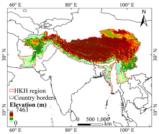
Figure 1.
Location of the study area and distribution of grassland types.
2.2. Normalized Difference Vegetation Index (NDVI)
The NDVI data used in the research were mainly derived from the MOD13A3 product of MODIS (Table 1), which was acquired from NASA EARTHDATA (https://earthdata.nasa.gov/ accessed on 1 March 2021) and used to estimate the fraction of photosynthetically active radiation (FPAR) absorbed by vegetation. The temporal resolution of NDVI data is monthly, and the spatial resolution is 1 km. We obtained the NDVI time series from 2001 to 2018 and then performed preprocessing, including splicing, cropping, projecting coordinates to the UTM WGS-1984 coordinate system, and resampling to 0.25° spatial resolution.

Table 1.
Description of the model input data set.
2.3. Meteorological Elements
Meteorological elements, including precipitation, air temperature, and solar radiation (Table 1), were derived from fifth-generation European Centre for Medium-Range Weather Forecasts (ECMWF) reanalysis data (ERA5) (https://cds.climate.copernicus.eu/ accessed on 1 March 2021), which are an alternative to ERA-Interim reanalysis. We obtained the monthly averaged reanalysis product type from the ERA5 dataset, including 2 m temperature, total precipitation, and surface solar radiation. These data were all stored in NC format, so we performed rasterization processing. We implemented the format conversion from NC to TIFF through Python, cropped the extents, reprojected the data to the UTM WGS-1984 coordinate system, and resampled the data to 0.25° spatial resolution with the nearest-neighbor method.
2.4. Soil Attribute Data
When inverting soil respiration, the variable soil organic carbon (SOC) density is essential, and its inversion needs to be calculated through soil attribute data. Soil attributes (Table 1) were derived from the Harmonized World Soil Database (HWSD) v.1.2 (http://www.fao.org/ accessed on 1 March 2021), which was developed by the International Institute of Applied Systems Analysis and Food and Agriculture Organization of the United Nations. The HWSD data are mainly composed of hwsd.bil, HWSD.mdb, and HWSD_META.mdb. Four soil parameters (bulk density, organic carbon, gravel content, and soil depth) are needed to calculate the SOC density. The soil attribute data were rasterized, cropped, resampled, and reprojected to make them consistent with NDVI and meteorological data.
2.5. Land Cover Type Data
The land cover type data were obtained from MCD12C1, MODIS, and NASA; the spatial resolution of these data is 0.05°, and the temporal resolution is yearly (Table 1). These data contain five land cover classification schemes, and the International Geosphere and Biosphere Program (IGBP) classification scheme was selected in our study. After the data were acquired, they needed to be cropped, reprojected, and resampled in Arc GIS 10.6 to obtain the input data required by the model with a 0.25°spatial resolution and UTM WGS-1984 geographic coordinate system. Finally, we chose grasslands and savannas in the 2010 IGBP classification as the grassland type input in the CASA model.
2.6. Net Primary Production (NPP) Estimation Model
The CASA model is a remote sensing-based process model. It performs well in long-term series and large-scale estimation of NPP [31,32]. The two indispensable components in the CASA model are absorbed photosynthetically active radiation (APAR) (MJ·m−2) and light use efficiency (LUE) factor ε (gC·MJ−1) [33,34,35]. For a particular pixel x at month t, NPP is calculated by the following equation:
where SOL is the surface solar radiation downwards (MJ·m−2). The constant 0.5 indicates that the solar energy used by vegetation photosynthesis is half of the total incident solar radiation [35].
The FPAR is a linear expression of NDVI and simple ratio (SR):
where and correspond to the 95% and 5% quantiles of the normal distribution of all pixels from monthly SR, respectively.
where T(x,t) is the temperature stress coefficients, and W(x,t) is the water stress coefficient. is the maximal LUE under ideal conditions with a value of 0.541 [36].
2.7. Geostatistical Model of Heterotrophic Respiration
The annual Rh is separated by annual total soil respiration using an empirical relationship through multiple analyses [37]. From multiple analysis, a global expression between Rh and soil respiration () was proposed:
The geostatistical model was developed on the basis of the global empirical soil respiration model proposed by Raich [38]. Then, Yu et al. [39] found that soil organic carbon density and soil respiration are strongly correlated, which is an additional control factor for the spatial change of soil respiration. Therefore, the soil organic carbon density variable was added to the global experience model. The parameters in the model were improved through measured data, and the following model was proposed [39]:
where is the mean soil respiration rates (gC·m−2·day−1); is the soil organic carbon density (kg·m−2); T is the mean monthly air temperature (℃); P is the mean monthly precipitation (cm); and , , P0, and K are all constant with values of 1.83, −0.006, 2.972, and 5.657, respectively [39].
Soil organic carbon density is directly related to soil properties [40,41], and its expression is as follows:
where BD is the soil bulk density (g·m−3); TOC represents the topsoil organic carbon (%); Depth is the depth of soil layer (cm), which is 20 cm in our study; and Gravel denotes the gravel content (%).
2.8. Trend Analysis of Grassland Net Ecosystem Production (NEP)
The ordinary least-squares method was selected to calculate a linear regression of grassland NEP over HKH in order to reveal the temporal trend of NEP. The formula is expressed as follows:
where slope is the interannual rate of NEP change; n is 18 for years from 2001 to 2018; i is 1 for the year 2001, 2 for the year 2002, and so on; and NEPi is the value of annual NEP in time of i year.
2.9. Partial Correlation Analysis
In order to evaluate the effects of a single climatic factor variable on NEP and to exclude interference from other climatic factors, we used a statistical partial correlation analysis method, which has been widely applied by many previous studies to explore the interaction between vegetation and a single climate element [42,43,44,45,46]. When two other climatic factors are used as dependent variables, the partial correlation coefficients of NEP and individual climatic factor can be calculated by the following equation:
where is the partial correlation coefficient between x and y excluding the impact of variable z; x and y are dependent variables, and z is the control variable. and are the simple correlation coefficients between x, y, and z, respectively. We took as an example to calculate the correlation coefficients between NEP and climatic elements:
where xi and yi are the annual grassland NEP and climate factor, respectively; and are the average NEP and mean climate factors from 2001 to 2018, respectively. Finally, a bilateral t-test was implemented to assess the significance of the partial correlation coefficients with a significance level of 0.05.
3. Results
3.1. Validation of the NPP and NEP Calculations
3.1.1. Validation of the NPP Values
We compared the monthly NPP estimated by the CASA model with the monthly NPP observed at the flux sites in the FLUXNET2015 database (https://fluxnet.org/data/fluxnet2015-dataset accessed on 1 March 2021). The flux site observed gross primary production (GPP), so this value needed to be multiplied by 0.55 (the ratio of NPP/GPP) to convert it into NPP [47]. For all sites (Table 2), the NPP measured at the site and estimated by the model through cross-validation had a regression coefficient of 0.74 and root mean square error (RMSE) of 25.65 gC·m−2 (Figure 2), which indicated a high precision of the CASA model estimation.
Table 2.
Description of flux tower sites in the Hindu Kush Himalayan (HKH) region.
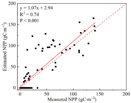
Figure 2.
Comparison of the estimated net primary production (NPP) with observed data from flux sites.
3.1.2. Reliability Analysis of the NEP Values
There are two main ways to verify the accuracy of regional NEP model simulations: one is to compare the simulated and measured data, and the other is to compare the simulation among different models [48]. Because the measured data in the HKH region are limited, we compared the average NEP values of the grassland ecosystems with prior studies. We mainly compared NEP values from the Qinghai–Tibet Plateau because prior studies are mostly concentrated there (Table 3). NEP and net ecosystem carbon exchange (NEE) are numerically equal [49,50,51]. There were differences between NEP values in this study and prior studies, but the NEP values of our study were basically within the range of values given in the published literature. This difference might have been mainly caused by the uncertainty of the Rh model, which was established by Bond-Lamberty et al. [37] through statistical analysis of measured data around the world. The following problems occurred: (1) The database used to establish the model had no measured data throughout the HKH region, which led to deviations in Rh when the model was applied in the HKH region. (2) The annual soil respiration (Rh) of the model was mainly derived from the expansion of the soil respiration (Rh) during the growing season, which would cause an overestimation of Rh. The soil microbial activity in the growing season and the decomposition ability were both strong, which would produce a large amount of carbon. In the nongrowing season, due to the decrease of temperature, the activity of microorganisms would weaken, and the carbon production would decrease. (3) A model based on a global scale might not be suitable for research on a regional scale. When the model was constructed, the strong spatial heterogeneity of the ground surface was not considered, so it might be biased when applied in the HKH region with strong heterogeneity.
Table 3.
Published studies of grassland ecosystem carbon sources/sinks on the Qinghai–Tibetan Plateau compared with our study.
3.2. Spatial Characteristics of NPP and NEP
3.2.1. Spatial Characteristics of NPP
Using the basic input data sets and the optimized CASA model, the grassland NPP in the HKH region from 2001 to 2018 was estimated and its distribution characteristics were analyzed (Figure 3a). Figure 3a shows that the NPP showed an increasing trend along the direction of Hindu Kush Himalayas from west to east, and the gradient distribution of NPP gradually but very obviously increased from northwest to southeast in the Qinghai–Tibet Plateau of China. The average grassland NPP throughout the HKH region was 294 ± 216 gC·m−2 during 2001 to 2018. In the western part of the HKH region, namely Afghanistan’s Hindu Kush Mountain and the western part of the Tibetan Plateau, NPP was less than 200 gC·m−2, accounting for 46.3% of the total grassland area. Areas with NPP greater than 600 gC·m−2 were mainly distributed in the eastern part of the Qinghai–Tibet Plateau, accounting for 12.4%. Judging from the difference in NPP between 2018 and 2001 (Figure 3b), the NPP of grassland in 2018 was higher than that in 2001, and most regions had a growing trend. Among them, regions with a growth magnitude of 0–100 gC·m−2 accounted for the highest proportion (59.8%), and the proportion of regions with NPP growth magnitude greater than 100 gC·m−2 was 9.1%. The growth trend showed that the hydrothermal conditions in 2018 were better than those in 2001, the photosynthesis of grassland was strong, and productivity was high.
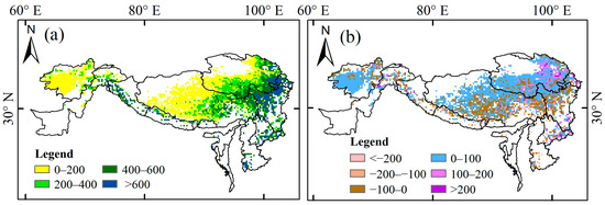
Figure 3.
The spatial pattern of (a) averaged grassland NPP during 2001–2018 and (b) NPP difference between 2018 and 2001.
3.2.2. Spatial Characteristics of NEP
The temporal and spatial distribution of NEP in the HKH region was determined by estimating NPP and soil respiration. A positive value of NEP indicates the area is a carbon sink, and a negative value indicates a carbon source [59]. From the perspective of spatial distribution characteristics (Figure 4a), the interannual NEP accumulation in the HKH region from 2001 to 2018 showed a significant upward trend from west to east, which was consistent with the trend of NPP. The grassland ecosystems in the HKH region showed a weak carbon sink, with an average NEP of 42 ± 197 gC·m−2, and the total net C sequestration was approximately 0.077 Pg C. In the past 18 years, the average amount of C sequestered by grassland ecosystems in the C sink area was 214.4 gC·m−2, and the total amount of carbon sequestered was approximately 0.187 Pg C. Carbon storage areas were mainly distributed in northern India, Nepal, and the southeastern Tibetan Plateau, accounting for approximately 52.2% of the total grassland area. At the same time, the average C emissions of grassland ecosystems in the carbon source sector was 116 gC·m−2, and the total C emissions were approximately 0.11 Pg C. The regions of carbon release were mainly concentrated in Afghanistan’s Hindu Kush Mountain and the western part of the Tibetan Plateau, accounting for about 47.8% of the total grassland area. Judging from the difference in NEP between 2018 and 2001 (Figure 4b), the carbon sequestration capacity of grassland in 2018 was stronger than in 2001. Regions with large fluctuations in NEP values were mainly distributed in the northeastern part of the Qinghai–Tibet Plateau, with an increase of more than 100 gC·m−2, and the NEP values in most regions fluctuated within plus or minus 100 gC·m−2.
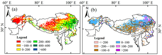
Figure 4.
The spatial pattern of (a) averaged grassland net ecosystem productivity (NEP) during 2001–2018 and (b) NEP difference between 2018 and 2001.
3.3. Temporal Trend of NPP and NEP
3.3.1. Interannual Variations
The mean annual NPP and NEP of grasslands in the HKH region showed a growth trend from 2001 to 2018 (Figure 5), and the growth trend of NPP was obvious, while NEP increased marginally. The variation of NPP ranged from 275.4 gC·m−2·yr−1 in 2001 to 303.6 gC·m−2·yr−1 in 2008 (range of 28.2 gC·m−2·yr−1), and the increment rate of NPP was 0.6 gC·m−2·yr−1. The magnitude of the fluctuation in NEP ranged from 27 gC·m−2·yr−1 in 2001 to 55.9 gC·m−2·yr−1 in 2008 (range of 28.8 gC·m−2·yr−1), and the growth rate of NEP was 0.2 gC·m−2·yr−1. In terms of time series, NEP and NPP were synchronized in amplitude and change, but it was difficult for Rh to synchronize with them. The magnitude of the fluctuation in Rh ranged from 247.6 gC·m−2·yr−1 in 2012 to 258.9 gC·m−2·yr−1 in 2016 (range of 11.3 gC·m−2·yr−1), and the growth rate of NEP was 0.4 gC·m−2·yr−1.
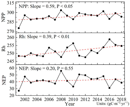
Figure 5.
Simulated trends in NPP, heterotrophic respiration (Rh), and NEP in HKH grassland ecosystems from 2001 to 2018.
3.3.2. Time Series Change Trend Distribution
The Mann–Kendall significance test was chosen to analyze the slope change trend of NEP and NPP, and significance level α = 0.05 (|z| ≥ 1.96) was selected to test the significance. There were obvious differences between NPP (Figure 6a) and NEP (Figure 6b), and the area of increase in NPP was more than that of NEP. The area that showed an increased trend in NPP (63.7%) was greater than that in NEP (53.4%). The area where NPP exhibited a significant increase accounted for approximately 13.1% of the total grassland area, and the area where NEP showed a significant increase accounted for about 8.6% of the total grassland area. The areas with significant increases of NPP and NEP were mainly concentrated in the south of the Afghanistan’s Hindu Kush Mountain and the northeast of the Qinghai–Tibet Plateau. The region where NEP showed a downward trend accounted for approximately 46.7% of the total grassland area and was mainly mapped to the southwest of the Qinghai–Tibet Plateau.
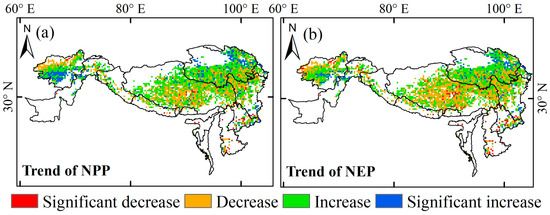
Figure 6.
The significance level of (a) NPP and (b) NEP interannual tendency.
3.4. The Impact of Climate on NPP and NEP
3.4.1. The Impact of Climate on NPP
To explore the main influencing factors that cause interannual changes of NPP in different regions, we calculated the partial correlation coefficients between NPP and precipitation, air temperature, and solar radiation (Figure 7a–c). Precipitation was the main limiting factor for NPP (Figure 7a). The area of steppe with NPP that was positively correlated with the precipitation was approximately 1.22 × 10⁶ km2, which accounted for about 67.3% of the total grassland area. The areas with a significant positive correlation between NPP and precipitation were mainly distributed in the Hindu Kush Mountains and the western areas of the Qinghai–Tibet Plateau. The partial correlation between NPP and temperature (Figure 7b) and solar radiation (Figure 7c) was insignificant over most of the area. The total areas of nonsignificant correlation were 1.68 × 10⁶ and 1.7 × 10⁶ km2, accounting for 92.1% and 93.5% of the total grassland area, respectively. The distribution of partial correlation showed that there was no strong correlation between NPP and temperature and solar radiation in most areas of the study area, which indicate that temperature and solar radiation are not the limiting climatic factors that affect the NPP of the HKH grassland ecosystem.
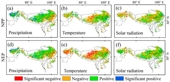
Figure 7.
Spatial patterns of the partial correlations between (a) NPP and precipitation, (b) NPP and temperature, (c) NPP and solar radiation, (d) NEP and precipitation, (e) NEP and temperature, and (f) NEP and solar radiation during 2001–2018.
3.4.2. The Impact of Climate on NEP
In order to explore the response of NEP to different climatic factors, we analyzed the partial correlation coefficients between NEP and annual accumulated precipitation, annual average air temperature, and annual total solar radiation from 2001 to 2018 and implemented a significance test (Figure 7d–f). Same as NPP, precipitation was also the dominant factor in NEP changes (Figure 7d). The area of steppe with NEP that was positively correlated with precipitation was approximately 1.15 × 10⁶ km2, which accounted for about 63.1% of the total HKH grassland area. In contrast to NPP, the partial correlation between NEP and temperature was mainly negative correlation with a partial correlation coefficient of −0.18 across the HKH grassland ecosystem (Figure 7e). The total area of negative correlation was 1.29 × 10⁶ km2, accounting for approximately 70.8% of the total grassland area, and the significant negative correlation accounted for 17.7% of the total grassland area, which was mainly distributed in the Hindu Kush Mountains and the western region of the Tibetan Plateau. The correlation between NEP and solar radiation (Figure 7f) was also significantly different from NPP and was mainly in the Hindu Kush Mountains. NEP and solar radiation had a positive correlation, while NPP was negatively correlated with solar radiation.
4. Discussion
4.1. Sources of Uncertainty
There are two main reasons for the differences in the tower-based flux and CASA estimates of NPP. One reason is the mismatch of the footprint; the flux measurement device is typically a tower-based eddy covariance system with a flux footprint of less than 1 km2, and they are subsamples of the CASA model pixel (0.25°) [60,61]. The other reason is that GPP measurements have systematic and random errors. Tower GPP is calculated as the difference between NEE and ecosystem respiration (Reco). Estimates of Reco at flux tower sites are typically created using nighttime fluxes of NEE [62]. However, the above-canopy fluxes are decoupled from the surface, leading to underestimates of nighttime respiration; thus, GPP exhibits deviations [63].
4.2. The Potential Effect of the NEP Spatial Distribution
The distribution of carbon sources and sinks throughout the HKH region were mainly affected by altitude and hydrothermal conditions, which is consistent with previous studies on the alpine grassland ecosystem of the Qinghai–Tibet Plateau [64,65]. As the altitude increased, the temperature decreased (Figure 8c), the solar radiation increased (Figure 8d), and the precipitation varied with altitude (Figure 8b). The precipitation at 0–2000 m was the highest, followed by that at 3000–4000 m, and the precipitation above 5000 m was the lowest. With the increase in altitude, the areas of grassland carbon sources and sinks both showed an increasing trend (Figure 8a), reaching a peak in the elevation range of 4000–5000 m, with a total net carbon sequestration of 77.25 kg C, mainly due to the widespread distribution of grassland (46.8%) in this altitude range. Above an altitude of 5000 m, the average NEP of grassland was the lowest because the area has limited precipitation and low temperature, which restricts the growth of grassland and reduces the carbon sequestration capacity of grassland. In the height range of 3000–4000 m, grasslands had the strongest carbon fixation capacity, with an average carbon fixation capacity of 283.4 gC·m−2. The average precipitation in this altitude range was relatively high at 880 mm, which provided sufficient water to the grasslands and resulted in strong photosynthesis, and these grasslands fixed a large amount of carbon from the atmosphere. In the height range of 0–2000 m, grassland had the strongest ability to release carbon into the atmosphere, with an average carbon emission of 151.3 gC·m−2. The high precipitation in this area reduces solar radiation, reduces photosynthesis, enhances respiration, and causes grassland to release carbon into the atmosphere. Among all the height classifications, the areas of the carbon sinks were larger than the areas of the carbon sources in the 3000–4000 m and 4000–5000 m height ranges, which were manifested as carbon sinks. In contrast, grasslands below 3000 m and above 5000 m were manifested as carbon sources.
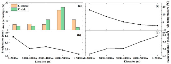
Figure 8.
Different elevation classifications of (a) C source or C sink area, (b) mean precipitation, (c) mean air temperature, and (d) mean solar radiation.
4.3. The Potential Effect of NEP Temporal Change
Precipitation is the main factor affecting NEP changes in alpine grassland ecosystems [62,64]. By analyzing the relationship between precipitation and NEP, it was found that changes in the two were not synchronized, and there was a lag effect. The peaks and valleys of NEP were always one year behind the time when the peaks and valleys of precipitation appeared. For example, the peak of precipitation appeared in 2010, while the peak of NEP appeared in 2011; the valley of precipitation appeared in 2006, and the valley of NEP appeared in 2007. By analyzing the partial correlation between NEP and the precipitation of the current year (Figure 7d–f) and the precipitation of the previous year (Figure 9a–c), it was found that the correlation between NEP and the precipitation of the previous year was strong and positive. The positive correlation covered 74% of the total area, which was 10.8% more than the positive correlation between NEP and the precipitation of the current year. This result also showed that if the precipitation in the previous year was sufficient, grassland growth would increase in the current year, and the grassland would have a strong carbon sequestration ability. The correlation between NEP and the temperature of the previous year was also stronger than that of the current year, with 44.1% of the area showing positive correlation, which was 14.9% more than the correlation between NEP and the temperature of the current year. Therefore, good hydrothermal conditions in the previous year will promote growth of NEP in the current year. The correlation between NEP and the solar radiation of the previous year showed an insignificant correlation (92.3%) in most areas, which was basically consistent with the correlation between NEP and the solar radiation of the current year (94.3%).
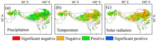
Figure 9.
Spatial patterns of the partial correlations between (a) NEP and precipitation, (b) NEP and temperature, (c) NEP and solar radiation of the previous year.
5. Conclusions
In this study, NEP of the HKH region from 2001 to 2018 was estimated based on the CASA model and geostatistical soil respiration model. We found that our results were within the range of the results of previous studies [52,53,54,55,56,57,58]. Although the uncertainty of the input data and the geostatistical soil respiration model resulted in deviations to the NEP estimation, our results reflected the temporal and spatial changes of the carbon sources/sinks in the HKH region. The grassland ecosystems had the potential to sequester carbon and showed an increasing trend from west to east. The grassland ecosystems were carbon sinks at 3000–5000 m, while carbon sources occurred at both lower than 3000 m and higher than 5000 m. Grassland had the strongest net carbon sequestration ability at 3000–4000 m, while grassland above 5000 m had the weakest net carbon sequestration capacity. Moreover, grassland NEP exhibited a stronger positive correlation with precipitation of the previous year than with precipitation of the current year. NEP was negatively correlated with temperature and not significantly correlated with solar radiation, and there was no obvious lag relationship. The above results based on large-scale analysis can help us understand the temporal and spatial changes of grassland ecosystem NEP in the HKH region and its response to climate change, which is of great significance to the development of grassland policies in the HKH region.
Author Contributions
D.G. designed this research experiment, performed analysis and verification, and drafted the manuscript. X.S. administrated the study, gave some constructive suggestions, and applied for funding for this study. R.H. participated in the design of the study and revised the draft to improve the presentation of this study. X.Z. offered some suggestions on visualization and the draft. S.C. participated in the realization and improvement of algorithm programming. Y.J. polished the pictures in the article. Y.Z. participated in editing the paper and checking for grammatical errors. X.C. provided guidance on thinking and logic. All authors have read and agreed to the published version of the manuscript.
Funding
This work was supported by funds for International Cooperation and Exchange of National Natural Science Foundation of China (Grant No. 31761143018), Special Project of National Natural Science Foundation of China (Grant No. 42041005), and the Second Tibetan Plateau Scientific Expedition and Research (STEP) program (Grant No. 2019QZKK0302).
Institutional Review Board Statement
Not applicable.
Informed Consent Statement
Not applicable.
Data Availability Statement
Data available in a publicly accessible repository.
Acknowledgments
The authors would like to thank the European Centre for Medium-Range Weather Forecasts for providing the climate dataset, the MODIS science teams for providing NDVI and land cover data, and the Food and Agriculture Organization of the United Nations for granting us access to the soil type data.
Conflicts of Interest
The authors declare no conflict of interest.
References
- Peichl, M.; Leahy, P.; Kiely, G. Six-year Stable Annual Uptake of Carbon Dioxide in Intensively Managed Humid Temperate Grassland. Ecosystems 2010, 14, 112–126. [Google Scholar] [CrossRef]
- Jongen, M.; Pereira, J.S.; Aires, L.M.I.; Pio, C.A. The effects of drought and timing of precipitation on the inter-annual variation in ecosystem-atmosphere exchange in a Mediterranean grassland. Agric. For. Meteorol. 2011, 151, 595–606. [Google Scholar] [CrossRef]
- Lei, T.; Feng, J.; Lv, J.; Wang, J.; Song, H.; Song, W.; Gao, X. Net Primary Productivity Loss under different drought levels in different grassland ecosystems. J. Environ. Manag. 2020, 274, 111144. [Google Scholar] [CrossRef] [PubMed]
- Kato, T.; Tang, Y.; Gu, S.; Hirota, M.; Du, M.; Li, Y.; Zhao, X. Temperature and biomass influences on interannual changes in CO2 exchange in an alpine meadow on the Qinghai-Tibetan Plateau. Glob. Chang. Biol. 2006, 12, 1285–1298. [Google Scholar] [CrossRef]
- Smith, P.; Lanigan, G.; Kutsch, W.L.; Buchmann, N.; Eugster, W.; Aubinet, M.; Ceschia, E.; Béziat, P.; Yeluripati, J.B.; Osborne, B.; et al. Measurements necessary for assessing the net ecosystem carbon budget of croplands. Agric. Ecosyst. Environ. 2010, 139, 302–315. [Google Scholar] [CrossRef]
- Scurlock, J.M.O.; Hall, D.O. The global carbon sink: A grassland perspective. Glob. Chang. Biol. 1998, 4, 229–233. [Google Scholar] [CrossRef]
- Suyker, A.E.; Verma, S.B.; Burba, G.G. Interannual variability in net CO2 exchange of a native tallgrass prairie. Glob. Chang. Biol. 2003, 9, 255–265. [Google Scholar] [CrossRef]
- Svejcar, T.; Angell, R.; Bradford, J.A.; Dugas, W.; Emmerich, W.; Frank, A.B.; Gilmanov, T.; Haferkamp, M.; Johnson, D.A.; Mayeux, H.; et al. Carbon Fluxes on North American Rangelands. Rangel. Ecol. Manag. 2008, 61, 465–474. [Google Scholar] [CrossRef]
- Zhang, L.; Wylie, B.K.; Ji, L.; Gilmanov, T.G.; Tieszen, L.L. Climate-Driven Interannual Variability in Net Ecosystem Exchange in the Northern Great Plains Grasslands. Rangel. Ecol. Manag. 2010, 63, 40–50. [Google Scholar] [CrossRef]
- Sun, S.; Che, T.; Li, H.; Wang, T.; Ma, C.; Liu, B.; Wu, Y.; Song, Z. Water and carbon dioxide exchange of an alpine meadow ecosystem in the northeastern Tibetan Plateau is energy-limited. Agric. For. Meteorol. 2019, 275, 283–295. [Google Scholar] [CrossRef]
- Lv, W.; Luo, C.; Zhang, L.; Niu, H.; Zhang, Z.; Wang, S.; Wang, Y.; Jiang, L.; Wang, Y.; He, J.; et al. Net neutral carbon responses to warming and grazing in alpine grassland ecosystems. Agric. For. Meteorol. 2020, 280, 107792. [Google Scholar] [CrossRef]
- Yang, F.; Zhang, Q.; Zhou, J.; Yue, P.; Wang, R.; Wang, S. East Asian summer monsoon substantially affects the inter-annual variation of carbon dioxide exchange in semi-arid grassland ecosystem in Loess Plateau. Agric. Ecosyst. Environ. 2019, 272, 218–229. [Google Scholar] [CrossRef]
- Meyers, T.P. A comparison of summertime water and CO2 fluxes over rangeland for well watered and drought conditions. Agric. For. Meteorol. 2001, 106, 205–214. [Google Scholar] [CrossRef]
- Zhang, L.; Guo, H.; Jia, G.; Wylie, B.; Gilmanov, T.; Howard, D.; Ji, L.; Xiao, J.; Li, J.; Yuan, W.; et al. Net ecosystem productivity of temperate grasslands in northern China: An upscaling study. Agric. For. Meteorol. 2014, 184, 71–81. [Google Scholar] [CrossRef]
- Tramontana, G.; Jung, M.; Schwalm, C.R.; Ichii, K.; Camps-Valls, G.; Ráduly, B.; Reichstein, M.; Arain, M.A.; Cescatti, A.; Kiely, G.; et al. Predicting carbon dioxide and energy fluxes across global FLUXNET sites with regression algorithms. Biogeosciences 2016, 13, 4291–4313. [Google Scholar] [CrossRef]
- Jung, M.; Reichstein, M.; Margolis, H.A.; Cescatti, A.; Richardson, A.D.; Arain, M.A.; Arneth, A.; Bernhofer, C.; Bonal, D.; Chen, J.; et al. Global patterns of land-atmosphere fluxes of carbon dioxide, latent heat, and sensible heat derived from eddy covariance, satellite, and meteorological observations. J. Geophys. Res. Space Phys. 2011, 116. [Google Scholar] [CrossRef]
- Zeng, J.; Matsunaga, T.; Tan, Z.-H.; Saigusa, N.; Shirai, T.; Tang, Y.; Peng, S.; Fukuda, Y. Global terrestrial carbon fluxes of 1999–2019 estimated by upscaling eddy covariance data with a random forest. Sci. Data 2020, 7, 313. [Google Scholar] [CrossRef]
- Laurin, G.V.; Vittucci, C.; Tramontana, G.; Ferrazzoli, P.; Guerriero, L.; Papale, D. Monitoring tropical forests under a functional perspective with satellite-based vegetation optical depth. Glob. Chang. Biol. 2020, 26, 3402–3416. [Google Scholar] [CrossRef]
- Shang, Z.; Degen, A.A.; Rafiq, M.K.; Squires, V.R. Correction to: Carbon Management for Promoting Local Livelihood in the Hindu Kush Himalayan (HKH) Region; Springer International Publishing: Berlin/Heidelberg, Germany, 2019; p. 1. [Google Scholar]
- Abbas, S.; Qamer, F.M.; Murthy, M.S.R.; Tripathi, N.K.; Ning, W.; Sharma, E.; Ali, G. Grassland Growth in Response to Climate Variability in the Upper Indus Basin, Pakistan. Climate 2015, 3, 697–714. [Google Scholar] [CrossRef]
- Panday, P.K.; Ghimire, B. Time-series analysis of NDVI from AVHRR data over the Hindu Kush–Himalayan region for the period 1982–2006. Int. J. Remote. Sens. 2012, 33, 6710–6721. [Google Scholar] [CrossRef]
- Qamer, F.M.; Xi, C.; Abbas, S.; Murthy, M.S.R.; Ning, W.; Anming, B. An Assessment of Productivity Patterns of Grass-Dominated Rangelands in the Hindu Kush Karakoram Region, Pakistan. Sustain. J. Rec. 2016, 8, 961. [Google Scholar] [CrossRef]
- Wu, J.; Wu, H.; Ding, Y.; Qin, J.; Li, H.; Liu, S.; Zeng, D. Interannual and seasonal variations in carbon exchanges over an alpine meadow in the northeastern edge of the Qinghai-Tibet Plateau, China. PLoS ONE 2020, 15, e0228470. [Google Scholar] [CrossRef] [PubMed]
- Liu, X.; Zhu, D.; Zhan, W.; Chen, H.; Zhu, Q.; Hao, Y.; Liu, W.; He, Y. Five-Year Measurements of Net Ecosystem CO2 Exchange at a Fen in the Zoige Peatlands on the Qinghai-Tibetan Plateau. J. Geophys. Res. Atmos. 2019, 124, 11803–11818. [Google Scholar] [CrossRef]
- Bin Hao, Y.; Cui, X.Y.; Wang, Y.F.; Mei, X.R.; Kang, X.M.; Wu, N.; Luo, P.; Zhu, D. Predominance of Precipitation and Temperature Controls on Ecosystem CO2 Exchange in Zoige Alpine Wetlands of Southwest China. Wetlands 2011, 31, 413–422. [Google Scholar] [CrossRef]
- Arun, A.; Ritu, V. Natural resource governance at multiple scales in the Hindu Kush Himalaya. ICIMOD Work. Pap. 2017, 4, 69. [Google Scholar]
- Ren, G.-Y.; Shrestha, A.B. Climate change in the Hindu Kush Himalaya. Adv. Clim. Chang. Res. 2017, 8, 137–140. [Google Scholar] [CrossRef]
- Wester, P.; Mishra, A.; Mukherji, A.; Shrestha, A.B. The Hindu Kush Himalaya Assessment: Mountains, Climate Change, Sustainability and People; Springer Nature: Berlin/Heidelberg, Germany, 2019. [Google Scholar]
- Gardelle, J.; Arnaud, Y.; Berthier, E. Contrasted evolution of glacial lakes along the Hindu Kush Himalaya mountain range between 1990 and 2009. Glob. Planet. Chang. 2011, 75, 47–55. [Google Scholar] [CrossRef]
- Bookhagen, B.; Burbank, D.W. Topography, relief, and TRMM-derived rainfall variations along the Himalaya. Geophys. Res. Lett. 2006, 33. [Google Scholar] [CrossRef]
- Xu, H.; Zhao, C.; Wang, X. Elevational differences in the net primary productivity response to climate constraints in a dryland mountain ecosystem of northwestern China. Land Degrad. Dev. 2020, 31, 2087–2103. [Google Scholar] [CrossRef]
- Guo, D.; Song, X.; Hu, R.; Cai, S.; Zhu, X.; Hao, Y. Grassland type-dependent spatiotemporal characteristics of productivity in Inner Mongolia and its response to climate factors. Sci. Total. Environ. 2021, 775, 145644. [Google Scholar] [CrossRef]
- Monteith, J.L. Solar Radiation and Productivity in Tropical Ecosystems. J. Appl. Ecol. 1972, 9, 747. [Google Scholar] [CrossRef]
- Field, C.B.; Randerson, J.T.; Malmström, C.M. Global net primary production: Combining ecology and remote sensing. Remote Sens. Environ. 1995, 51, 74–88. [Google Scholar] [CrossRef]
- Potter, C.S.; Randerson, J.T.; Field, C.B.; Matson, P.A.; Vitousek, P.M.; Mooney, H.A.; Klooster, S.A. Terrestrial ecosystem production: A process model based on global satellite and surface data. Glob. Biogeochem. Cycles 1993, 7, 811–841. [Google Scholar] [CrossRef]
- Yu, D.; Shi, P.; Shao, H.; Zhu, W.; Pan, Y. Modelling net primary productivity of terrestrial ecosystems in East Asia based on an improved CASA ecosystem model. Int. J. Remote. Sens. 2009, 30, 4851–4866. [Google Scholar] [CrossRef]
- Bond-Lamberty, B.; Wang, C.; Gower, S.T. A global relationship between the heterotrophic and autotrophic components of soil respiration? Glob. Chang. Biol. 2004, 10, 1756–1766. [Google Scholar] [CrossRef]
- Raich, J.W.; Potter, C.S.; Bhagawati, D. Interannual variability in global soil respiration, 1980–1994. Glob. Chang. Biol. 2002, 8, 800–812. [Google Scholar] [CrossRef]
- Yu, G.; Zheng, Z.; Wang, Q.; Fu, Y.; Zhuang, J.; Sun, X.; Wang, Y. Spatiotemporal Pattern of Soil Respiration of Terrestrial Ecosystems in China: The Development of a Geostatistical Model and Its Simulation. Environ. Sci. Technol. 2010, 44, 6074–6080. [Google Scholar] [CrossRef] [PubMed]
- Xia, X.; Yang, Z.; Xue, Y.; Shao, X.; Yu, T.; Hou, Q. Spatial analysis of land use change effect on soil organic carbon stocks in the eastern regions of China between 1980 and 2000. Geosci. Front. 2017, 8, 597–603. [Google Scholar] [CrossRef]
- Yu, T.; Fu, Y.; Hou, Q.; Xia, X.; Yan, B.; Yang, Z. Soil organic carbon increase in semi-arid regions of China from 1980s to 2010s. Appl. Geochem. 2020, 116, 104575. [Google Scholar] [CrossRef]
- Peng, S.; Piao, S.; Ciais, P.; Myneni, R.B.; Chen, A.; Chevallier, F.; Dolman, A.J.; Janssens, I.A.; Peñuelas, J.; Zhang, G.; et al. Asymmetric effects of daytime and night-time warming on Northern Hemisphere vegetation. Nat. Cell Biol. 2013, 501, 88–92. [Google Scholar] [CrossRef]
- Beer, C.; Reichstein, M.; Tomelleri, E.; Ciais, P.; Jung, M.; Carvalhais, N.; Rödenbeck, C.; Arain, M.A.; Baldocchi, D.; Bonan, G.B.; et al. Terrestrial gross carbon dioxide uptake: Global distribution and covariation with climate. Science 2010, 329, 834–838. [Google Scholar] [CrossRef] [PubMed]
- Wu, D.H.; Zhao, X.; Liang, S.L.; Zhou, T.; Huang, K.C.; Tang, B.J.; Zhao, W.Q. Time-lag effects of global vegetation responses to climate change. Glob. Chang. Biol. 2015, 21, 3520–3531. [Google Scholar] [CrossRef] [PubMed]
- Wen, Y.; Liu, X.; Pei, F.; Li, X.; Du, G. Non-uniform time-lag effects of terrestrial vegetation responses to asymmetric warming. Agric. For. Meteorol. 2018, 252, 130–143. [Google Scholar] [CrossRef]
- Xu, G.; Zhang, H.; Chen, B.; Zhang, H.; Innes, J.L.; Wang, G.; Yan, J.; Zheng, Y.; Zhu, Z.; Myneni, R.B. Changes in Vegetation Growth Dynamics and Relations with Climate over China’s Landmass from 1982 to 2011. Remote Sens. 2014, 6, 3263–3283. [Google Scholar] [CrossRef]
- Zhang, Y.; Yu, G.; Yang, J.; Wimberly, M.C.; Zhang, X.; Tao, J.; Jiang, Y.; Zhu, J. Climate-driven global changes in carbon use efficiency. Glob. Ecol. Biogeogr. 2013, 23, 144–155. [Google Scholar] [CrossRef]
- Zhou, X.; Yu, F.; Cao, G.; Yang, W.; Zhou, Y. Spatiotemporal features of carbon source-sink and its relationship with climate factors in Qinghai-Tibet Plateau grassland ecosystem during 2001–2015. Res. Soil Water Conserv. 2019, 26, 76–81. [Google Scholar]
- Chai, X.; Shi, P.; Song, M.; Zong, N.; He, Y.; Zhao, G.; Zhang, X. Carbon flux phenology and net ecosystem productivity simulated by a bioclimatic index in an alpine steppe-meadow on the Tibetan Plateau. Ecol. Model. 2019, 394, 66–75. [Google Scholar] [CrossRef]
- Elsgaard, L.; Görres, C.-M.; Hoffmann, C.C.; Blicher-Mathiesen, G.; Schelde, K.; Petersen, S.O. Net ecosystem exchange of CO2 and carbon balance for eight temperate organic soils under agricultural management. Agric. Ecosyst. Environ. 2012, 162, 52–67. [Google Scholar] [CrossRef]
- Li, H.; Zhang, F.; Li, Y.; Wang, J.; Zhang, L.; Zhao, L.; Cao, G.; Zhao, X.; Du, M. Seasonal and inter-annual variations in CO2 fluxes over 10 years in an alpine shrubland on the Qinghai-Tibetan Plateau, China. Agric. For. Meteorol. 2016, 228–229, 95–103. [Google Scholar] [CrossRef]
- Wang, H.; Ma, M.; Wang, X.; Tan, J.; Gen, L.; Yu, W. Carbon flux variation characteristics and its influencing factors in an alpine meadow ecosystem on eastern Qinghai-Tibetan plateau. J. Arid Land Resour. Environ. Earth Sci. 2014, 28, 50–56. [Google Scholar]
- Pei, Z.; Zhou, C.; Ouyang, H.; Yang, W. A carbon budget of alpine steppe area in the Tibetan Plateau. Geogr. Res. 2010, 29, 102–110. [Google Scholar]
- Zhao, L.; Li, Y.; Xu, S.; Zhou, H.; Gu, S.; Yu, G.; Zhao, X. Diurnal, seasonal and annual variation in net ecosystem CO2 exchange of an alpine shrubland on Qinghai-Tibetan plateau. Glob. Chang. Biol. 2006, 12, 1940–1953. [Google Scholar] [CrossRef]
- Wang, Y.; Ma, Y.; Li, H.; Yuan, L. Carbon and water fluxes and their coupling in an alpine meadow ecosystem on the northeastern Tibetan Plateau. Theor. Appl. Clim. 2020, 142, 1–18. [Google Scholar] [CrossRef]
- Niu, B.; He, Y.; Zhang, X.; Du, M.; Shi, P.; Sun, W. CO2 Exchange in an Alpine Swamp Meadow on the Central Tibetan Plateau. Wetlands 2017, 37, 525–543. [Google Scholar] [CrossRef]
- Wang, S.; Zhang, Y.; Lu, S.; Su, P.; Shang, L.; Li, Z. Biophysical regulation of carbon fluxes over an alpine meadow ecosystem in the eastern Tibetan Plateau. Int. J. Biometeorol. 2015, 60, 801–812. [Google Scholar] [CrossRef]
- Wang, B.; Jin, H.; Li, Q.; Chen, D.; Zhao, L.; Tang, Y.; Kato, T.; Gu, S. Diurnal and Seasonal Variations in the Net Ecosystem CO2 Exchange of a Pasture in the Three-River Source Region of the Qinghai−Tibetan Plateau. PLoS ONE 2017, 12, e0170963. [Google Scholar] [CrossRef] [PubMed]
- Luyssaert, S.; Schulze, E.-D.; Börner, A.; Knohl, A.; Hessenmöller, D.; Law, B.E.; Ciais, P.; Grace, J.D. Old-growth forests as global carbon sinks. Nat. Cell Biol. 2008, 455, 213–215. [Google Scholar] [CrossRef] [PubMed]
- Dai, E.; Huang, Y.; Wu, Z.; Zhao, D. Analysis of spatio-temporal features of a carbon source/sink and its relationship to climatic factors in the Inner Mongolia grassland ecosystem. J. Geogr. Sci. 2016, 26, 297–312. [Google Scholar] [CrossRef]
- Li, F.; Kustas, W.P.; Anderson, M.C.; Prueger, J.H.; Scott, R.L. Effect of remote sensing spatial resolution on interpreting tower-based flux observations. Remote. Sens. Environ. 2008, 112, 337–349. [Google Scholar] [CrossRef]
- Zhang, T.; Zhang, Y.; Xu, M.; Zhu, J.; Chen, N.; Jiang, Y.; Huang, K.; Zu, J.; Liu, Y.; Yu, G. Water availability is more important than temperature in driving the carbon fluxes of an alpine meadow on the Tibetan Plateau. Agric. For. Meteorol. 2018, 256-257, 22–31. [Google Scholar] [CrossRef]
- Heinsch, F.; Zhao, M.; Running, S.; Kimball, J.; Nemani, R.; Davis, K.; Bolstad, P.; Cook, B.; Desai, A.; Ricciuto, D.; et al. Evaluation of remote sensing based terrestrial productivity from MODIS using regional tower eddy flux network observations. IEEE Trans. Geosci. Remote Sens. 2006, 44, 1908–1925. [Google Scholar] [CrossRef]
- Zhuang, Q.; He, J.; Lu, Y.; Ji, L.; Xiao, J.; Luo, T. Carbon dynamics of terrestrial ecosystems on the Tibetan Plateau during the 20th century: An analysis with a process-based biogeochemical model. Glob. Ecol. Biogeogr. 2010, 19, 649–662. [Google Scholar] [CrossRef]
- Piao, S.; Tan, K.; Nan, H.; Ciais, P.; Fang, J.; Wang, T.; Vuichard, N.; Zhu, B. Impacts of climate and CO2 changes on the vegetation growth and carbon balance of Qinghai–Tibetan grasslands over the past five decades. Glob. Planet. Chang. 2012, 98-99, 73–80. [Google Scholar] [CrossRef]
Publisher’s Note: MDPI stays neutral with regard to jurisdictional claims in published maps and institutional affiliations. |
© 2021 by the authors. Licensee MDPI, Basel, Switzerland. This article is an open access article distributed under the terms and conditions of the Creative Commons Attribution (CC BY) license (http://creativecommons.org/licenses/by/4.0/).