TNNG: Total Nuclear Norms of Gradients for Hyperspectral Image Prior

Abstract

We introduce a novel regularization function for hyperspectral image (HSI), which is based on the nuclear norms of gradient images. Unlike conventional low-rank priors, we achieve a gradient-based low-rank approximation by minimizing the sum of nuclear norms associated with rotated planes in the gradient of a HSI. Our method explicitly and simultaneously exploits the correlation in the spectral domain as well as the spatial domain. Our method exploits the low-rankness of a global region to enhance the dimensionality reduction by the prior. Since our method considers the low-rankness in the gradient domain, it more sensitively detects anomalous variations. Our method achieves high-fidelity image recovery using a single regularization function without the explicit use of any sparsity-inducing priors such as ${\ell }_0$, ${\ell }_1$ and total variation (TV) norms. We also apply this regularization to a gradient-based robust principal component analysis and show its superiority in HSI decomposition. To demonstrate, the proposed regularization is validated on a variety of HSI reconstruction/decomposition problems with performance comparisons to state-of-the-art methods its superior performance.

1. Introduction

Convex optimization techniques have gained broad interest in many hyperspectral image processing applications including image restoration [1,2,3,4,5,6,7,8], decomposition [9,10], unmixing [11,12,13], classification [14,15], and target detection [16]. The success of such tasks strongly depends on regularization, which is based on a priori information of a latent clear image. Total Variation (TV) is one of the exemplary models often used for regularization in convex optimization approaches [17,18,19,20,21]. Some convex optimization methods specializing in low-rank regularization have been proposed in recent years [22,23]; these use the spectral information directly and achieve high-quality image restoration.

In this paper, we propose a regularization scheme that directly and simultaneously considers correlation in the spatio-spectral domains. We name the regularization function as Total Nuclear Norms of Gradients (TNNG), which calculates nuclear norms for all planes in the gradient domain of a HSI to exploit correlations in all spatio-spectral directions and obtains a low-rank approximation of its structure. The function utilizes the a priori property, where each gradient possesses strong inter-band correlation, and it directly controls each gradient that expresses smoothness in the spatial direction and correlation in the spectral direction. We also apply the TNNG regularization scheme to a Gradient-based Robust Principal Component Analysis (GRPCA) and show its superior performance in image decomposition.

There are many methods with low-rank priors [18,22,23], but there are few approaches that exploit low-rankness in global regions of the $xz$ and $yz$ planes (x, y, and z indicate horizontal/vertical/spectral directions, respectively). Recently, a joint approach of low-rank restoration and non-local filtering has been proposed [24]. The method achieves high-fidelity restoration by incorporating subspace learning with the non-local filtering. However, this method works well only for image denoising tasks.

The efficiency of our method is due to the following three features:

• Exploiting the low-rankness of a global region (i.e., a high-dimensional matrix) allows us to enhance the dimensionality reduction by the prior.
• Inherently, HSIs have little correlation in oblique directions within the $xz$ and $yz$ planes. We efficiently exploit this property through our regularization.
• Since our method considers the low-rankness in the gradient domain, not the low-rankness in the image domain, it more sensitively detects anomalous variations.

Another notable property in our regularization is that our method does not explicitly use any sparsity-inducing norms such as ${\ell }_0$ or ${\ell }_1$ norms. Taking the nuclear norms on all the $xz$ and $yz$ planes, we implicitly reduce variations on spatial domains as well. In the end, our simple regularization simultaneously exploits the low-rank property and sparsity in spatial variations as a single function. Due to this property, we can apply our regularization function to RPCA as well as the HSI restoration, and unlike conventional methods, our method is efficient for various applications in image restoration and decomposition.

We solve convex optimization problems using primal-dual splitting (PDS) [25] and apply it to various hyperspectral image processing tasks. Experimentally, we conduct HSI restoration, RPCA-based image decomposition, and HSI pansharpening problems as examples to confirm their performance.

This paper is organized as follows. After reviewing conventional methods on HSI processing in Section 2, we describe the details of the algorithm and the solutions for the proposed optimization problem in Section 3. In Section 4, we present several experiments on image reconstruction/decomposition to illustrate the superiority of the proposed method. Section 6 presents a summary of this study and future prospects.

2. Related Work

Many restoration methods based on TV for multi-channel images have previously been proposed [17,18,19,20,21]. Yuan et al. [21] proposed a hyperspectral TV (HTV), which is an expansion of the TV model to HSI. They also proposed a spectral-spatial adaptive HTV (SSAHTV), which introduces adaptive weights to HTV. SSAHTV uses spectral information for its weighting and shows superior performance over HTV. The structure tensor TV (STV) [17] was proposed for multi-channel images and considers low-rankness of gradient vectors in local regions. Furthermore, its arranged version (ASTV) was proposed in [18] and outperforms STV in some image restoration problems. These methods show high performance on HSI restoration, but they only consider correlation in the spatial domain explicitly. Meanwhile, spectral information is limited to indirect use in these regularization schemes; therefore, it is relatively prone to excessive smoothing because of the substantial impact received from the spatial properties. Some of them consider the spectral gradients, few methods exploit the low-rankness in the gradient domain by a single regularization function.

It is well known that there exist high correlations among HSI along the spectral direction, especially in aerial images, as each spectral signature can be well represented by a linear combination of a small number of pure spectral endmembers, which induces the low-rank property. Low-rank matrix recovery (LRMR) [23], which utilizes the low-rankness of local blocks in HSI, has been shown to have higher performance than SSAHTV and even VBM3D [26], which is one of the most superior methods for non-local noise reduction. Furthermore, the spatio-spectral TV (SSTV) was proposed in [27]; it applies TV to the HSI gradient in the spectral direction. It is a regularization scheme that indirectly considers spatial correlation through the application of TV to the spectral gradient. Although it is a simple method, SSTV is confirmed to be superior to LRMR. Contrary to STV and ASTV, noise tends to remain in the restoration results of LRMR and SSTV because of the weak influence from the spatial properties. The methods such as LRTV [22], HSSTV [28], and LRTDTV [29] attempt to improve the performance of STV, SSTV, and its variants by introducing new regularization. However, future tasks are still to be elucidated, such as over-smoothing.

Recent DNN-based approaches have been successful for 2D image restoration tasks such as super-resolution [30,31]. Although there are a few successful methods for HSI such as [32,33,34,35,36], the superiority of DNN for HSI restoration is limited. This is due to the following reasons: (1) Acquiring high-quality large HSI data sets is not straightforward. (2) DNN-based methods are sensitive to attributes such as the number of spectral bands, spectral ranges of wavelengths, types of sensor, and thus such a domain mismatch in attributes between training and test data often degrades performance. On the other hand, regularization-based approaches like ours are more flexible and can be applied to many restoration tasks, such as restoration, unmixing, and classification.

3. Proposed Method

3.1. Low-Rankness of Spectral Gradients

Letting the spatial coordinates be x, y, and spectral coordinates z, we define “front” as the direction in which we view the $xy$ planes along the z axis. The “top” and “side” are defined as the directions in which we view the $xz$ and $yz$ planes, respectively. Here, we define $\mathbf{x}\in {\mathbb{R}}^{n_v\times n_h\times B}$ to be a HSI with an image size of $n_v\times n_h$ and number of bands B. Furthermore, we define ${\mathbf{G}}_v\in {\mathbb{R}}^{n_h\times B\times 3n_v}$ to be a combined 3D gradient image where the three gradient images for $\mathbf{x}$ (w.r.t. vertical, horizontal, and spectral directions) observed from the top view, are concatenated to form a 3D cuboid. Similarly, we define ${\mathbf{G}}_h\in {\mathbb{R}}^{n_v\times B\times 3n_h}$ to be the 3D cuboid of the gradient images observed from the side view. We will explain detailed formulation in Section 3.2.

We represent the sum of ranks for all single-structure planes in ${\mathbf{G}}_v$ and ${\mathbf{G}}_h$ as follows:

$$\sum _{i=1}^{3n_v}\mathrm{rank}\left({\mathbf{G}}_v^{\left(i\right)}\right)+\sum _{i=1}^{3n_h}\mathrm{rank}\left({\mathbf{G}}_h^{\left(i\right)}\right),$$

(1)

where ${\mathbf{G}}_v^{\left(i\right)}\in {\mathbb{R}}^{n_h\times B}$ represents the i-th plane extracted from ${\mathbf{G}}_v$ and similarly ${\mathbf{G}}_h^{\left(i\right)}\in {\mathbb{R}}^{n_v\times B}$ is the i-th plane extracted from ${\mathbf{G}}_h$. Given that ${\mathbf{G}}_v$, which is observed from the top view, possesses size B in the vertical direction and size $n_v$ in depth, the total number of ${\mathbf{G}}_v^{\left(i\right)}$ is $3n_v$. Similarly, the total number of ${\mathbf{G}}_h^{\left(i\right)}$ is $3n_h$.

Since (1) uses rank with a discrete value and is a non-convex function, the minimization problem with (1) is NP-hard. Therefore, we incorporate the nuclear norm (${\parallel ·\parallel }_{*}={\sum }_k{\sigma }_k$), which is the optimal relaxation of the rank constraint, and substitute

$$\mathcal{L}\left(\mathbf{x}\right)=\sum _{i=1}^{3n_v}\parallel {\mathbf{G}}_v^{\left(i\right)}{\parallel }_{*}+\sum _{i=1}^{3n_h}{\parallel {\mathbf{G}}_h^{\left(i\right)}\parallel }_{*},$$

(2)

for (1). We refer to this regularization as the Total Nuclear Norms of Gradients (TNNG). TNNG is used as regularization to approximate ${\mathbf{G}}_v$ and ${\mathbf{G}}_h$ through a low-rank model.

Figure 1 shows diagonal matrices ${\mathbf{S}}_{•}^{\left(i\right)}$ of the image PaviaU, where singular value decomposition (${\mathbf{G}}_{•}^{\left(i\right)}={\mathbf{U}}_{•}^{\left(i\right)}{\mathbf{S}}_{•}^{\left(i\right)}{\mathbf{V}}_{•}^{\left(i\right)\top }$) is performed on some ${\mathbf{G}}_{•}^{\left(i\right)}(•:v\mathrm{or}h)$ of the HSI. The red lines show enlarged views of the top 15 singular values. ${\mathbf{S}}_{•}^{\left(i\right)}$ possesses singular values of ${\mathbf{G}}_{•}^{\left(i\right)}$ as diagonal components. In any diagonal matrix ${\mathbf{S}}_{•}^{\left(i\right)}$, we can observe that there is energy concentration to a handful of singular values, and most of the values are close to 0. This observation shows that ${\mathbf{G}}_{•}^{\left(i\right)}$ approximately forms a low-rank structure. In ${\mathbf{S}}_h^{\left(i\right)}$ of the noisy HSI, there is energy dispersion, which violates the low-rank structure, while there is energy concentration in a portion of ${\mathbf{S}}_h^{\left(i\right)}$ in the restored HSI. Therefore, one can see that the restored image has a low-rank structure and more closely approximates the original HSI. As this property can be seen in most images, it is expected that the low-rank approximation in the gradient domain using TNNG will work for restoration.

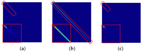
Figure 1. An example for the diagonal matrix ${\mathbf{S}}_h^{\left(i\right)}$ of PaviaU in which the diagonal elements are singular values of ${\mathbf{G}}_h^{\left(i\right)}$. The three images show ${\mathbf{S}}_h^{\left(i\right)}$ of the original input, noisy image, and restoration results, respectively. (a) original, (b) noisy, (c) restoration.

3.2. TNNG Regularization

In this section, we design ${\mathbf{G}}_v$ and ${\mathbf{G}}_h$, and specifically formulate TNNG. We redefine a HSI with an image size of $N=n_v·n_h$ and the number of bands B as a vector $\mathbf{x}={[{\mathbf{x}}_1^{\top },\dots ,{\mathbf{x}}_B^{\top }]}^{\top }\in {\mathbb{R}}^{NB}$. A single plane ${\mathbf{x}}_j\in {\mathbb{R}}^N(j=1,\dots ,B)$ represents the image of the j-th band of $\mathbf{x}$, and ${\mathbf{x}}_j^{\top }$ represents the transposed ${\mathbf{x}}_j$.

We define the linear operator $\mathbf{D}$ to find the spatio-spectral gradients. Let the vertical and horizontal difference operators be ${\mathbf{D}}_v,{\mathbf{D}}_h\in {\mathbb{R}}^{NB\times NB}$, and let the spectral difference operator be ${\mathbf{D}}_s\in {\mathbb{R}}^{NB\times NB}$ as:

$${\mathbf{D}}_s=\left[\begin{array}{cccccc}\hfill -\mathbf{I}& \hfill \mathbf{I}& \hfill \mathbf{O}& \hfill \dots & \hfill \dots & \hfill \mathbf{O}\\ \hfill \mathbf{O}& \hfill -\mathbf{I}& \hfill \mathbf{I}& \hfill \mathbf{O}& \hfill \dots & \hfill \mathbf{O}\\ \hfill ⋮& \hfill \ddots & \hfill \ddots & \hfill \ddots & \hfill & \hfill ⋮\\ \hfill ⋮& \hfill & \hfill \mathbf{O}& \hfill -\mathbf{I}& \hfill \mathbf{I}& \hfill \mathbf{O}\\ \hfill \mathbf{O}& \hfill & & \hfill \ddots & \hfill -\mathbf{I}& \hfill \mathbf{I}\\ \hfill \mathbf{I}& \hfill \mathbf{O}& \hfill \dots & \hfill \dots & \hfill \mathbf{O}& \hfill -\mathbf{I}\end{array}\right],$$

(3)

where $\mathbf{I}\in {\mathbb{R}}^{N\times N}$ is an identity matrix, and $\mathbf{O}\in {\mathbb{R}}^{N\times N}$ is a zero matrix. Using these single-direction operators, we define the spatio-spectral difference operator $\mathbf{D}\in {\mathbb{R}}^{3NB\times NB}$ as follows:

$$\mathbf{D}={\left[{\mathbf{D}}_v^{\top }{\mathbf{D}}_h^{\top }{\mathbf{D}}_s^{\top }\right]}^{\top }.$$

(4)

Then, we calculate the spatio-spectral gradients of HSI, $\mathbf{D}\mathbf{x}\in {\mathbb{R}}^{3NB}$. This procedure is illustrated in the left part of Figure 2. ${\mathbf{D}}_v\mathbf{x}$, ${\mathbf{D}}_h\mathbf{x}$, and ${\mathbf{D}}_s\mathbf{x}$$\in {\mathbb{R}}^{NB}$ represent the vectorized versions of the three 3D components (vertical, horizontal, and spectral, respectively) of the gradient image.

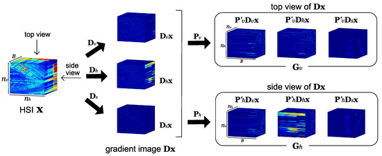
Figure 2. Gradient images and rotation by ${\mathbf{P}}_v^{\prime }$ and ${\mathbf{P}}_h^{\prime }$.

Next, we introduce two operators ${\mathbf{P}}_v,{\mathbf{P}}_h\in {\mathbb{R}}^{3NB\times 3NB}$, which rearrange pixels so that the upper and side planes of $\mathbf{D}\mathbf{x}$ are located in the front:

$${\mathbf{P}}_v=\left[\begin{array}{ccc}\hfill {\mathbf{P}}_v^{\prime }& \hfill \mathbf{O}& \hfill \mathbf{O}\\ \hfill \mathbf{O}& \hfill {\mathbf{P}}_v^{\prime }& \hfill \mathbf{O}\\ \hfill \mathbf{O}& \hfill \mathbf{O}& \hfill {\mathbf{P}}_v^{\prime }\end{array}\right],{\mathbf{P}}_h=\left[\begin{array}{ccc}\hfill {\mathbf{P}}_h^{\prime }& \hfill \mathbf{O}& \hfill \mathbf{O}\\ \hfill \mathbf{O}& \hfill {\mathbf{P}}_h^{\prime }& \hfill \mathbf{O}\\ \hfill \mathbf{O}& \hfill \mathbf{O}& \hfill {\mathbf{P}}_h^{\prime }\end{array}\right],$$

(5)

where ${\mathbf{P}}_v^{\prime }$ is a matrix that rotates each of ${\mathbf{D}}_v\mathbf{x}$, ${\mathbf{D}}_h\mathbf{x}$, and ${\mathbf{D}}_s\mathbf{x}$ such that the $yz$, $xy$, and $zx$ planes face in the directions of “front”, “side”, and “top”, respectively, and similarly ${\mathbf{P}}_h^{\prime }$ has a role of rotating the cuboids such that the $zx$, $xy$, and $yz$ planes faces in the directions of “front”, “side”, and “top”, respectively (see the right part of Figure 2). In addition, we use the operator $\mathrm{\Gamma }$, which converts a vector into a 3D cuboid, to rewrite the vectors ${\mathbf{P}}_v\mathbf{D}\mathbf{x}\mathrm{and}{\mathbf{P}}_h\mathbf{D}\mathbf{x}\in {\mathbb{R}}^{3NB}$ as follows:

$$\begin{array}{c}\hfill \begin{array}{cc}& {\mathbf{P}}_v\mathbf{D}\mathbf{x}\in {\mathbb{R}}^{3NB}\mapsto {\mathbf{G}}_v=\mathrm{\Gamma }\left({\mathbf{P}}_v\mathbf{D}\mathbf{x}\right)\in {\mathbb{R}}^{n_h\times B\times 3n_v},\hfill \\ & {\mathbf{P}}_h\mathbf{D}\mathbf{x}\in {\mathbb{R}}^{3NB}\mapsto {\mathbf{G}}_h=\mathrm{\Gamma }\left({\mathbf{P}}_h\mathbf{D}\mathbf{x}\right)\in {\mathbb{R}}^{n_v\times B\times 3n_h}.\hfill \end{array}\end{array}$$

(6)

The right side of Figure 2 shows an image diagram when ${\mathbf{G}}_v$ and ${\mathbf{G}}_h$ are designed using $\mathbf{D}$, ${\mathbf{P}}_v$, and ${\mathbf{P}}_h$. Rewriting (2) using $\mathbf{D}$, ${\mathbf{P}}_v$, and ${\mathbf{P}}_h$ defined by (4) and (5), TNNG in (2) is expressed as follows:

$$\mathcal{L}\left(\mathbf{x}\right)=\sum _{i=1}^{3n_v}\parallel \mathrm{\Gamma }{\left({\mathbf{P}}_v\mathbf{D}\mathbf{x}\right)}^{\left(i\right)}{\parallel }_{*}+\sum _{i=1}^{3n_h}{\parallel \mathrm{\Gamma }{\left({\mathbf{P}}_h\mathbf{D}\mathbf{x}\right)}^{\left(i\right)}\parallel }_{*},$$

(7)

where $\parallel \mathrm{\Gamma }{\left({\mathbf{P}}_v\mathbf{D}\mathbf{x}\right)}^{\left(i\right)}{\parallel }_{*}$ represents the nuclear norm of the i-th plane in the 3D cuboid $\mathrm{\Gamma }\left({\mathbf{P}}_v\mathbf{D}\mathbf{x}\right)$.

3.3. HSI Restoration Model

In this section, we formulate an image restoration problem. The HSI observation model is represented by the following equation using an original image $\mathbf{x}\in {\mathbb{R}}^{NB}$ and an observed image $\mathbf{y}\in {\mathbb{R}}^K$:

$$\mathbf{y}=\mathbf{A}\mathbf{x}+\mathbf{n},$$

(8)

where $\mathbf{A}\in {\mathbb{R}}^{K\times NB}(K\le NB)$ is the linear operator that represents deterioration (for example, it represents random sampling in the case of compressed sensing [37,38]), and $\mathbf{n}\in {\mathbb{R}}^K$ represents additive noise. Based on the observation model, the convex optimization problem for the HSI restoration using TNNG can be formulated as follows:

$$\underset{\mathbf{x}}{min}\lambda \mathcal{L}\left(\mathbf{x}\right)+{\mathcal{F}}_{\mathrm{y}}\left(\mathbf{A}\mathbf{x}\right)\mathrm{s}.\mathrm{t}.\mathbf{x}\in \mathcal{C}.$$

(9)

Here, $\lambda$ is the weight of TNNG, $\mathcal{C}={[{\rho }_{\min },{\rho }_{\max }]}^{NB}$ represents the box constraint of the pixel values in the closed convex set, and ${\rho }_{\min }$, ${\rho }_{\max }$ represent the minimum and maximum pixel values taken by $\mathbf{x}$, respectively. In addition, ${\mathcal{F}}_{\mathrm{y}}$ is a data-fidelity function, and it is necessary to select a suitable ${\mathcal{F}}_{\mathrm{y}}$ depending on the observed distribution of noise. We assume that the additive noise follows a Gaussian distribution, and thus we use the ${\ell }_2$-norm to express the convex optimization problem of Problem (9) as follows:

$$\underset{\mathbf{x}}{min}\lambda \mathcal{L}\left(\mathbf{x}\right)+\frac{1}{2}{\parallel \mathbf{A}\mathbf{x}-\mathbf{y}\parallel }_2^2\mathrm{s}.\mathrm{t}.\mathbf{x}\in \mathcal{C}.$$

(10)

3.4. Gradient-Based Robust Principal Component Analysis

We apply TNNG to 3D Robust Principal Component Analysis (RPCA). RPCA [39] has been used in many computer vision and image processing applications. The goal of RPCA in the case of 2D images is to decompose an image matrix $\mathbf{Y}\in {\mathbb{R}}^{M\times N}$ to a low-rank component $\mathbf{L}\in {\mathbb{R}}^{M\times N}$ and a sparse residual $\mathbf{S}\in {\mathbb{R}}^{M\times N}$ by solving the following equation:

$$\begin{array}{ccc}& & \underset{\mathbf{L},\mathbf{S}}{min}{\lambda \parallel \mathbf{L}\parallel }_{*}+{\parallel \mathbf{S}\parallel }_1\mathrm{s}.\mathrm{t}.\mathbf{Y}=\mathbf{L}+\mathbf{S}.\hfill \end{array}$$

(11)

We extend this to HSI image decomposition by applying TNNG as follows:

$$\underset{\mathbf{x},\mathbf{s}}{min}\lambda \mathcal{L}\left(\mathbf{x}\right)+{\parallel \mathbf{s}\parallel }_1\mathrm{s}.\mathrm{t}.\mathbf{y}=\mathbf{x}+\mathbf{s},\mathbf{x},\mathbf{s}\in \mathcal{C}.$$

(12)

By solving (12), we achieve the decomposition of the observed measurement $\mathbf{y}\in {\mathbb{R}}^{NB}$ as $\mathbf{y}=\mathbf{x}+\mathbf{s}$, where $\mathbf{x}\in {\mathbb{R}}^{NB}$ is low-rank in the gradient domain, and $\mathbf{s}\in {\mathbb{R}}^{NB}$ is the sparse component. The two constraints in (12) guarantee the exact reconstruction and the reasonable range of pixel values. Unlike the existing 3D RPCA methods [40,41], we analyze the low-rankness of an HSI in the gradient domain. As it is gradient-based, it also has the capability of excluding sparse anomalies more sensitively, so it is expected that the performance of the decomposition improves. We call this Gradient-based RPCA (GRPCA). This problem is also convex optimization, and thus one efficiently obtains a global optimum solution by convex optimization algorithms.

3.5. HSI Pansharpening Model

Pan sharpening is a technique for generating an HSI with high spatial and spectral resolutions by combining a panchromatic image (pan image) with a high spatial resolution and a HSI with a high spectral resolution. It is important in the field of remote sensing and earth observation.

Let $\mathbf{x}\in {\mathbb{R}}^{NB}$ be a true HSI with high spatial resolution, ${\mathbf{y}}_{hs}\in {\mathbb{R}}^{N^{\prime }B}(N^{\prime }<N)$ be an observed HSI with low spatial resolution, and ${\mathbf{y}}_{pan}\in {\mathbb{R}}^N$ be an observed gray-scale pan image. The observation model of HSI for pansharpening can be formulated as follows:

$${\mathbf{y}}_{hs}=\mathbf{S}\mathbf{B}\mathbf{x}+{\mathbf{n}}_{hs},{\mathbf{y}}_{pan}=\mathbf{R}\mathbf{x}+{\mathbf{n}}_{pan},$$

(13)

where $\mathbf{B}\in {\mathbb{R}}^{NB\times NB}$ and $\mathbf{S}\in {\mathbb{R}}^{N^{\prime }\times NB}$ represent the lowpass operator and sub-sampling operator, respectively. The matrix $\mathbf{R}\in {\mathbb{R}}^{N\times NB}$ represents an average operator. In our setting, we simply average all bands to makes a gray-scale image. ${\mathbf{n}}_{hs}\in {\mathbb{R}}^{N^{\prime }B}$ and ${\mathbf{n}}_{pan}\in {\mathbb{R}}^N$ represent additive noise.

The goal of the pansharpening problem is to recover the full spatial and spectral resolution image $\mathbf{x}$, which is similar to $\mathbf{u}$, from the observed two images ${\mathbf{y}}_{hs}$ and ${\mathbf{y}}_{pan}$. Using the proposed regularization defined by (7), we adopt the following convex optimization problem to estimate $\mathbf{x}$.

$$\begin{array}{cccc}\hfill & \underset{\mathbf{x}}{min}\hfill & \hfill & \mathcal{L}\left(\mathbf{x}\right)\hfill \\ \hfill & \mathrm{subject}\mathrm{to}\hfill & \hfill & \parallel \mathbf{S}\mathbf{B}\mathbf{x}-{\mathbf{y}}_{hs}{\parallel }_2\le {ϵ}_{hs},\hfill \\ \hfill & \hfill & & \parallel \mathbf{R}\mathbf{x}-{\mathbf{y}}_{pan}{\parallel }_2\le {ϵ}_{pan},\hfill \\ & \hfill & & \mathbf{x}\in {[0,1]}^{NB},\hfill \end{array}$$

(14)

where ${ϵ}_{hs}$ and ${ϵ}_{pan}$ are user-defined parameters that controls the fidelity of $\mathbf{x}$.

3.6. Optimization

In this study, we adopt primal-dual splitting (PDS) [25] to solve the convex optimization problems in (10), (12), and (14). PDS is an iterative algorithm to solve a convex optimization problem of the form

$$\underset{\mathbf{x}}{min}F\left(\mathbf{x}\right)+G\left(\mathbf{x}\right)+H\left(\mathbf{L}\mathbf{x}\right),$$

(15)

where F represents a convex function where the gradient is $\beta$-Lipschitz continuous and differentiable, G and H represent the non-smooth convex functions where the proximity operator can be efficiently calculated, and $\mathbf{L}$ is a linear operator. Proximity operator [42,43] is defined using the lower semi-continuous convex function $\psi$ and index $\gamma >0$, as

$${\mathrm{prox}}_{\gamma \psi }\left(\mathbf{v}\right)=\underset{\mathbf{z}}{\arg \min }\psi \left(\mathbf{z}\right)+\frac{1}{2\gamma }{\parallel \mathbf{z}-\mathbf{v}\parallel }_2^2.$$

(16)

The PDS algorithm to solve Problem (15) is given as follows [25,44,45]:

$$⌊\begin{array}{c}{\mathbf{x}}^{(k+1)}={\mathrm{prox}}_{{\gamma }_{1}G}({\mathbf{x}}^{\left(k\right)}-{\gamma }_1(\nabla F\left({\mathbf{x}}^{\left(k\right)}\right)+{\mathbf{L}}^{\top }{\mathbf{z}}^{\left(k\right)})),\hfill \\ \mathbf{v}\leftarrow {\mathbf{z}}^{\left(k\right)}+{\gamma }_2\mathbf{L}(2{\mathbf{x}}^{(k+1)}-{\mathbf{x}}^{\left(k\right)}),\hfill \\ {\mathbf{z}}^{(k+1)}=\mathbf{v}-{\gamma }_2{\mathrm{prox}}_{\frac{1}{{\gamma }_2}H}\left(\frac{1}{{\gamma }_2}\mathbf{v}\right)\hfill \end{array}$$

(17)

where $\nabla F$ is the gradient of F, $\mathbf{x}$ is the primal variable, $\mathbf{z}$ is the dual variable of $\mathbf{L}\mathbf{x}$, $\mathbf{v}$ is the mediator variable to calculate $\mathbf{z}$, and the superscript $\left(k\right)$ indicates the k-th iteration. The algorithm converges to an optimal solution of Problem (15) by iteratively solving (17) under appropriate conditions on ${\gamma }_1$ and ${\gamma }_2$.

In the paper, we explain only the procedure to solve Problem (10), but one can also solve Problem (12) and (14) in a similar way. The respective algorithms are shown in shown in Algorithm 1 and Algorithm 2. To apply PDS to Problem (10), we define the indicator function ${\iota }_{\mathcal{C}}$ with a closed convex set as follows:

$${\iota }_{\mathcal{C}}\left(\mathbf{x}\right)=\left\{\begin{array}{cc}0,\hfill & \mathbf{x}\in \mathcal{C},\hfill \\ +\infty ,\hfill & \mathrm{otherwise}.\hfill \end{array}\right.$$

(18)

We use this indicator function to turn Problem (10) into a convex optimization problem with no apparent constraints as follows:

$$\underset{\mathbf{x}}{min}\lambda \mathcal{L}\left(\mathbf{x}\right)+\frac{1}{2}{\parallel \mathbf{A}\mathbf{x}-\mathbf{y}\parallel }_2^2+{\iota }_{\mathcal{C}}\left(\mathbf{x}\right).$$

(19)

Problem (19) is formed by the convex functions allowing efficient calculation of the proximity operator. To represent (19) in the same format as Problem (15), to which PDS can be applied, we separate each term of Problem (19) into F, G, and H as follows:

$$\begin{array}{cc}\hfill & F\left(\mathbf{x}\right)=\frac{1}{2}{\parallel \mathbf{A}\mathbf{x}-\mathbf{y}\parallel }_2^2,G\left(\mathbf{x}\right)={\iota }_{\mathcal{C}}\left(\mathbf{x}\right),\hfill \\ \hfill & H\left(\mathbf{L}\mathbf{x}\right)=\lambda \mathcal{L}\left(\mathbf{x}\right)=\lambda (\sum _{i=1}^{3n_v}\parallel \mathrm{\Gamma }{\left({\mathbf{P}}_v\mathbf{D}\mathbf{x}\right)}^{\left(i\right)}{\parallel }_{*}+\sum _{i=1}^{3n_h}\parallel \mathrm{\Gamma }{\left({\mathbf{P}}_h\mathbf{D}\mathbf{x}\right)}^{\left(i\right)}{\parallel }_{*}).\hfill \end{array}$$

(20)

The function $F:{\mathbb{R}}^{NB}\to \mathbb{R}$ is formed only by the differentiable ${\ell }_2$-norm, and thus its gradient $\nabla F$ is obtained by

$$\nabla F\left(\mathbf{x}\right)={\mathbf{A}}^{\top }(\mathbf{A}\mathbf{x}-\mathbf{y}).$$

(21)

The function $G:{\mathbb{R}}^{NB}\to \mathbb{R}\cup \{\infty \}$ becomes the indicator function ${\iota }_{\mathcal{C}}$. The ${\mathrm{prox}}_{{\gamma }_{1}G}$ of (17) becomes ${\mathrm{prox}}_{{\gamma }_1{\iota }_{\mathcal{C}}}:{\mathbb{R}}^{NB}\to {\mathbb{R}}^{NB}$, the projection that is the proximity operator to the box constraint. If we set the projection to ${\mathrm{prox}}_{{\gamma }_1{\iota }_{\mathcal{C}}}\left(\mathbf{x}\right)=P_{\mathcal{C}}\left(\mathbf{x}\right)$, then the projection $P_{\mathcal{C}}\left(\mathbf{x}\right)$ can be given, for $i=1,\dots ,NB$, as follows:

$${\left[P_{\mathcal{C}}\left(\mathbf{x}\right)\right]}_i=\left\{\begin{array}{cc}{\rho }_{\min },\hfill & \mathrm{if}{\mathit{x}}_{\mathit{i}}<{\rho }_{\min },\hfill \\ x_i,\hfill & \mathrm{if}{\rho }_{\min }\le {\mathit{x}}_{\mathit{i}}\le {\rho }_{\max },\hfill \\ {\rho }_{\max },\hfill & \mathrm{if}{\mathit{x}}_{\mathit{i}}>{\rho }_{\max }.\hfill \end{array}\right.$$

(22)

We perform the operation separately for each element $x_i$ in $\mathbf{x}$. The function $H:{\mathbb{R}}^{3NB+3NB}\to \mathbb{R}$ corresponds to the regularization function, and the dual variable $\mathbf{z}$ and linear operator $\mathbf{L}$ can be given as follows:

$$\begin{array}{cc}\hfill \mathbf{z}& ={[{\mathbf{z}}_1^{\top },{\mathbf{z}}_2^{\top }]}^{\top }\mapsto \sum _{i=1}^{3n_v}\parallel \mathrm{\Gamma }{\left({\mathbf{z}}_1\right)}^{\left(i\right)}{\parallel }_{*}+\sum _{i=1}^{3n_h}{\parallel \mathrm{\Gamma }{\left({\mathbf{z}}_2\right)}^{\left(i\right)}\parallel }_{*},\hfill \\ \hfill \mathbf{L}& :{\mathbb{R}}^{NB}\to {\mathbb{R}}^{3NB+3NB},\mathbf{x}\mapsto ({\mathbf{P}}_v\mathbf{D}\mathbf{x},{\mathbf{P}}_h\mathbf{D}\mathbf{x}).\hfill \end{array}$$

(23)

Here, ${\mathbf{z}}_1$ and ${\mathbf{z}}_2$ are dual variables corresponding to ${\mathbf{P}}_v\mathbf{D}\mathbf{x}$ and ${\mathbf{P}}_h\mathbf{D}\mathbf{x}$, respectively. Given that TNNG uses a nuclear norm, the ${\mathrm{prox}}_{\frac{1}{{\gamma }_2}H}$ performs soft-thresholding with respect to singular values of each matrix ${\mathbf{G}}_{•}^{\left(i\right)}=\mathrm{\Gamma }{\left({\mathbf{P}}_{•}\mathbf{D}\mathbf{x}\right)}^{\left(i\right)}(•:v\mathrm{or}h)$ in (7). Here, the singular value decomposition of ${\mathbf{G}}_{•}^{\left(i\right)}$ becomes ${\mathbf{G}}_{•}^{\left(i\right)}={\mathbf{U}}_{•}^{\left(i\right)}{\mathbf{S}}_{•}^{\left(i\right)}{\mathbf{V}}_{•}^{\left(i\right)\top }$. Thus, the proximity operator, ${\mathrm{prox}}_{\frac{1}{{\gamma }_2}{\parallel ·\parallel }_{*}}$ is given as follows:

$$\begin{array}{cc}\hfill & {\mathrm{prox}}_{\frac{1}{{\gamma }_2}{\parallel ·\parallel }_{*}}\left({\mathbf{G}}_{•}^{\left(i\right)}\right)={\mathbf{U}}_{•}^{\left(i\right)}{\tilde{\mathbf{S}}}_{•}^{\left(i\right)}{\mathbf{V}}_{•}^{\left(i\right)\top },\hfill \\ \hfill & {\tilde{\mathbf{S}}}_{•}^{\left(i\right)}=\mathrm{diag}(max\{{\sigma }_1^{\left(i\right)}-\gamma ,0\},\cdots ,max\{{\sigma }_M^{\left(i\right)}-\gamma ,0\}),\hfill \end{array}$$

(24)

where $\mathrm{diag}(·)$ represents a diagonal matrix with diagonal elements $(·)$, and M is the maximum number of singular values.

Based on the above discussion, we can solve the convex optimization problem of Problem (10) using PDS, whose steps are shown in Algorithm 3. The calculation for the projection $P_{\mathcal{C}}$ (step 4) is indicated in (22), and the proximity operator of nuclear norms (steps 7, 8) is given by (24). We set the stopping criterion to $|x^{(k+1)}-x^{\left(k\right)}|/|x^{(k+1)}|<1e-5$.

Algorithm 1 PDS Algorithm for Solving Problem (12)

1: input : ${\mathbf{x}}^{\left(0\right)}$, ${\mathbf{s}}^{\left(0\right)}$ 2: set : ${\gamma }_1$, ${\gamma }_2$ and initial values for ${\mathbf{z}}_1^{\left(0\right)}$, ${\mathbf{z}}_2^{\left(0\right)}$, ${\mathbf{z}}_3^{\left(0\right)}$, ${\mathbf{z}}_4^{\left(0\right)}$ are given. 3: while a stopping criterion is not satisfied do 4:  ${\mathbf{x}}^{(k+1)}=P_{\mathcal{C}}\{{\mathbf{x}}^{\left(k\right)}-{\gamma }_1({\mathbf{D}}^{\top }({\mathbf{P}}_v^{\top }{\mathbf{z}}_1^{\left(k\right)}+{\mathbf{P}}_h^{\top }{\mathbf{z}}_2^{\left(k\right)})+{\mathbf{z}}_4^{\left(k\right)})\}$; 5:  ${\mathbf{s}}^{(k+1)}=P_{\mathcal{C}}\{{\mathbf{s}}^{\left(k\right)}-{\gamma }_1({\mathbf{z}}_3^{\left(k\right)}+{\mathbf{z}}_4^{\left(k\right)})\}$; 6:  ${\mathbf{v}}_1\leftarrow {\mathbf{z}}_1^{\left(k\right)}+{\gamma }_2{\mathbf{P}}_v\mathbf{D}(2{\mathbf{x}}^{(k+1)}-{\mathbf{x}}^{\left(k\right)})$; 7:  ${\mathbf{v}}_2\leftarrow {\mathbf{z}}_2^{\left(k\right)}+{\gamma }_2{\mathbf{P}}_h\mathbf{D}(2{\mathbf{x}}^{(k+1)}-{\mathbf{x}}^{\left(k\right)})$; 8:  ${\mathbf{v}}_3\leftarrow {\mathbf{z}}_3^{\left(k\right)}+{\gamma }_2(2{\mathbf{s}}^{(k+1)}-{\mathbf{s}}^{\left(k\right)})$; 9:  ${\mathbf{v}}_4\leftarrow {\mathbf{z}}_4^{\left(k\right)}+{\gamma }_2(2{\mathbf{s}}^{(k+1)}-{\mathbf{s}}^{\left(k\right)})$; 10:  ${\mathbf{z}}_1^{(k+1)}={\mathbf{v}}_1-{\gamma }_2{\mathrm{prox}}_{\frac{1}{{\gamma }_2}{\parallel ·\parallel }_{*}}\left(\frac{1}{{\gamma }_2}{\mathbf{v}}_1\right)$; 11:  ${\mathbf{z}}_2^{(k+1)}={\mathbf{v}}_2-{\gamma }_2{\mathrm{prox}}_{\frac{1}{{\gamma }_2}{\parallel ·\parallel }_{*}}\left(\frac{1}{{\gamma }_2}{\mathbf{v}}_2\right)$; 12:  ${\mathbf{z}}_3^{(k+1)}={\mathbf{v}}_3-{\gamma }_2{\mathrm{prox}}_{\frac{1}{{\gamma }_2}{\parallel ·\parallel }_1}\left(\frac{1}{{\gamma }_2}{\mathbf{v}}_3\right)$; 13:  ${\mathbf{z}}_4^{(k+1)}={\mathbf{v}}_4-{\gamma }_2{\mathrm{prox}}_{\frac{1}{{\gamma }_2}{\iota }_{\left\{\mathbf{y}\right\}}}\left(\frac{1}{{\gamma }_2}{\mathbf{v}}_4\right)$; 14:  Update iteration: $k\leftarrow k+1$; 15: end while 16: output : ${\mathbf{x}}^{(k+1)}$

We turn Problem (12) into a convex optimization problem with no apparent constraints as follows:

$$\underset{\mathbf{x}}{min}\lambda \mathcal{L}\left(\mathbf{x}\right)+{\parallel \mathbf{s}\parallel }_1+{\iota }_{\mathbf{y}}(\mathbf{x}+\mathbf{s})+{\iota }_{\mathcal{C}}\left(\mathbf{x}\right)+{\iota }_{\mathcal{C}}\left(\mathbf{s}\right).$$

(25)

Problem (25) is formed by the convex functions allowing efficient calculation of the proximity operator. To represent (25) in the same format as Problem (15), to which PDS can be applied, we separate each term of Problem (25) into F, G, and H as follows:

$$\begin{array}{cc}\hfill & F\left(\mathbf{x}\right)=0,G\left(\mathbf{x}\right)={\iota }_{\mathcal{C}}\left(\mathbf{x}\right)+{\iota }_{\mathcal{C}}\left(\mathbf{s}\right),\hfill \\ \hfill & H\left(\mathbf{L}\mathbf{x}\right)=\lambda (\sum _{i=1}^{3n_v}\parallel \mathrm{\Gamma }{\left({\mathbf{P}}_v\mathbf{D}\mathbf{x}\right)}^{\left(i\right)}{\parallel }_{*}+\sum _{i=1}^{3n_h}\parallel \mathrm{\Gamma }{\left({\mathbf{P}}_h\mathbf{D}\mathbf{x}\right)}^{\left(i\right)}{\parallel }_{*}{)+\parallel \mathbf{s}\parallel }_1+{\iota }_{\mathbf{y}}(\mathbf{x}+\mathbf{s}).\hfill \end{array}$$

(26)

Steps 12 of Algorithm 1 is the proximity operator, ${\mathrm{prox}}_{\frac{1}{{\gamma }_2}{\parallel ·\parallel }_1}$ is given as follows:

$${\left[{prox}_{{\gamma \parallel ·\parallel }_1}\left(\mathbf{x}\right)\right]}_i=sgn\left(x_i\right)max\left\{\left|x_i\right|-\gamma ,0\right\},$$

(27)

for i = 1,...,NB, where $sgn(·)$ denotes the sign of $(·)$, ${prox}_{\gamma {\iota }_{\left\{\mathbf{y}\right\}}}(·)$ is $\mathbf{y}$.

We turn Problem (14) into a convex optimization problem with no apparent constraints as follows:

$$\underset{\mathbf{x}}{min}\mathcal{L}\left(\mathbf{x}\right)+{\iota }_{{\mathcal{B}}_{2,{\epsilon }_{hs}}^{{\mathrm{y}}_{hs}}}\left(\mathbf{SBx}\right)+{\iota }_{{\mathcal{B}}_{2,{\epsilon }_{pan}}^{{\mathrm{y}}_{pan}}}\left(\mathbf{Rx}\right)+{\iota }_{\mathcal{C}}\left(x\right)$$

(28)

Problem (28) is formed by the convex functions allowing efficient calculation of the proximity operator. To represent (28) in the same format as Problem (15), to which PDS can be applied, we separate each term of Problem (28) into F, G, and H as follows:

$$\begin{array}{cc}\hfill & F\left(\mathbf{x}\right)=0,G\left(\mathbf{x}\right)={\iota }_{\mathcal{C}}\left(\mathbf{x}\right),\hfill \\ \hfill & H\left(\mathbf{L}\mathbf{x}\right)=\sum _{i=1}^{3n_v}\parallel \mathrm{\Gamma }{\left({\mathbf{P}}_v\mathbf{D}\mathbf{x}\right)}^{\left(i\right)}{\parallel }_{*}+\sum _{i=1}^{3n_h}{\parallel \mathrm{\Gamma }{\left({\mathbf{P}}_h\mathbf{D}\mathbf{x}\right)}^{\left(i\right)}\parallel }_{*}+{\iota }_{{\mathcal{B}}_{2,{\epsilon }_{hs}}^{{\mathrm{y}}_{hs}}}\left(\mathbf{SBx}\right)+{\iota }_{{\mathcal{B}}_{2,{\epsilon }_{pan}}^{{\mathrm{y}}_{pan}}}\left(\mathbf{R}\right).\hfill \end{array}$$

(29)

Algorithm 2 PDS Algorithm for Solving Problem (14)

1: input : ${\mathbf{x}}^{\left(0\right)}$ 2: set : ${\gamma }_1$, ${\gamma }_2$ and initial values for ${\mathbf{z}}_1^{\left(0\right)}$, ${\mathbf{z}}_2^{\left(0\right)}$, ${\mathbf{z}}_3^{\left(0\right)}$, ${\mathbf{z}}_4^{\left(0\right)}$ are given. 3: while a stopping criterion is not satisfied do 4:  ${\mathbf{x}}^{(k+1)}=P_{\mathcal{C}}\{{\mathbf{x}}^{\left(k\right)}-{\gamma }_1({\mathbf{D}}^{\top }({\mathbf{P}}_v^{\top }{\mathbf{z}}_1^{\left(k\right)}+{\mathbf{P}}_h^{\top }{\mathbf{z}}_2^{\left(k\right)})+{\mathbf{B}}^{\top }{\mathbf{S}}^{\top }{\mathbf{z}}_3^{\left(k\right)}+{\mathbf{R}}^{\top }{\mathbf{z}}_4^{\left(k\right)})\}$; 5:  ${\mathbf{v}}_1\leftarrow {\mathbf{z}}_1^{\left(k\right)}+{\gamma }_2{\mathbf{P}}_v\mathbf{D}(2{\mathbf{x}}^{(k+1)}-{\mathbf{x}}^{\left(k\right)})$; 6:  ${\mathbf{v}}_2\leftarrow {\mathbf{z}}_2^{\left(k\right)}+{\gamma }_2{\mathbf{P}}_h\mathbf{D}(2{\mathbf{x}}^{(k+1)}-{\mathbf{x}}^{\left(k\right)})$; 7:  ${\mathbf{v}}_3\leftarrow {\mathbf{z}}_3^{\left(k\right)}+{\gamma }_2\mathbf{S}\mathbf{B}(2{\mathbf{x}}^{(k+1)}-{\mathbf{x}}^{\left(k\right)})$; 8:  ${\mathbf{v}}_4\leftarrow {\mathbf{z}}_4^{\left(k\right)}+{\gamma }_2\mathbf{R}(2{\mathbf{x}}^{(k+1)}-{\mathbf{x}}^{\left(k\right)})$; 9:  ${\mathbf{z}}_1^{(k+1)}={\mathbf{v}}_1-{\gamma }_2{\mathrm{prox}}_{\frac{1}{{\gamma }_2}{\parallel ·\parallel }_{*}}\left(\frac{1}{{\gamma }_2}{\mathbf{v}}_1\right)$; 10:  ${\mathbf{z}}_2^{(k+1)}={\mathbf{v}}_2-{\gamma }_2{\mathrm{prox}}_{\frac{1}{{\gamma }_2}{\parallel ·\parallel }_{*}}\left(\frac{1}{{\gamma }_2}{\mathbf{v}}_2\right)$; 11:  ${\mathbf{z}}_3^{(k+1)}={\mathbf{v}}_3-{\gamma }_2{\mathrm{prox}}_{\frac{1}{{\gamma }_2}{\mathcal{B}}_{2,{\epsilon }_{hs}}^{{\mathrm{y}}_{hs}}}\left(\frac{1}{{\gamma }_2}{\mathbf{v}}_3\right)$; 12:  ${\mathbf{z}}_4^{(k+1)}={\mathbf{v}}_4-{\gamma }_2{\mathrm{prox}}_{\frac{1}{{\gamma }_2}{\mathcal{B}}_{2,{\epsilon }_{pan}}^{{\mathrm{y}}_{pan}}}\left(\frac{1}{{\gamma }_2}{\mathbf{v}}_4\right)$; 13:  Update iteration: $k\leftarrow k+1$; 14: end while 15: output : ${\mathbf{x}}^{(k+1)}$

Steps 12 and 13 of Algorithm 2 is updated by using the following ${\ell }_2$ ball projection:

$${prox}_{\gamma ,{\mathcal{B}}_{2,\epsilon }^{\mathrm{v}}\left(\mathbf{x}\right)}=\left\{\begin{array}{cc}\mathbf{x},\hfill & \mathrm{if}\mathbf{x}\in {\mathcal{B}}_{2,\epsilon }^{\mathrm{v}},\hfill \\ \mathbf{v}+\frac{\epsilon \left(\mathbf{x}-\mathbf{v}\right)}{{∥\mathbf{x}-\mathbf{v}∥}_2},\hfill & \mathrm{otherwise},\hfill \end{array}\right.$$

(30)

where $ϵ$ is the radius of the ${\ell }_2$-norm sphere. And, ${\mathcal{B}}_{2,\epsilon }^{\mathbf{v}}$ is define as ${\mathcal{B}}_{2,\epsilon }^{\mathbf{v}}:=\{\mathbf{x}\in {\mathbb{R}}^{NB}{|\parallel \mathbf{x}-\mathbf{v}\parallel }_2\le \epsilon \}$.

Algorithm 3: PDS Algorithm for Solving Problem (10)

1: input : ${\mathbf{x}}^{\left(0\right)}$ 2: set : ${\gamma }_1$, ${\gamma }_2$ and initial values for ${\mathbf{z}}_1^{\left(0\right)}$, ${\mathbf{z}}_2^{\left(0\right)}$ are given. 3: whilea stopping criterion is not satisfieddo 4:  ${\mathbf{x}}^{(k+1)}=P_{\mathcal{C}}\{{\mathbf{x}}^{\left(k\right)}-{\gamma }_1({\mathbf{A}}^{\top }(\mathbf{A}{\mathbf{x}}^{\left(k\right)}-\mathbf{y})+{\mathbf{D}}^{\top }({\mathbf{P}}_v^{\top }{\mathbf{z}}_1^{\left(k\right)}+{\mathbf{P}}_h^{\top }{\mathbf{z}}_2^{\left(k\right)}))\}$; 5:  ${\mathbf{v}}_1\leftarrow {\mathbf{z}}_1^{\left(k\right)}+{\gamma }_2{\mathbf{P}}_v\mathbf{D}(2{\mathbf{x}}^{(k+1)}-{\mathbf{x}}^{\left(k\right)})$; 6:  ${\mathbf{v}}_2\leftarrow {\mathbf{z}}_2^{\left(k\right)}+{\gamma }_2{\mathbf{P}}_h\mathbf{D}(2{\mathbf{x}}^{(k+1)}-{\mathbf{x}}^{\left(k\right)})$; 7:  ${\mathbf{z}}_1^{(k+1)}={\mathbf{v}}_1-{\gamma }_2{\mathrm{prox}}_{\frac{1}{{\gamma }_2}H}\left(\frac{1}{{\gamma }_2}{\mathbf{v}}_1\right)$; 8:  ${\mathbf{z}}_2^{(k+1)}={\mathbf{v}}_2-{\gamma }_2{\mathrm{prox}}_{\frac{1}{{\gamma }_2}H}\left(\frac{1}{{\gamma }_2}{\mathbf{v}}_2\right)$; 9:  Update iteration: $k\leftarrow k+1$; 10: end while 11: output : ${\mathbf{x}}^{(k+1)}$

4. Results

To show the effectiveness of the proposed method, we conducted several experiments on compressed sensing (CS), signal decomposition, and pansharpening. There results were compared the results with some conventional methods.

We used PSNR and Structural Similarity Index (SSIM) [46] as objective measures of CS and signal decomposition, and SAM [47], ERGAS [48], and Q2n [49] for pansharpening. The evaluation methods for SAM, ERGAS, and Q2n are explained below. $\mathbf{y}\in {\mathbb{R}}^{NB}$ is a grandtruth image, $\mathbf{x}\in {\mathbb{R}}^{NB}$ is a restored image.

• SAM is defined as follows:

  $$\begin{array}{c}\hfill SAM\left(\mathbf{x},\mathbf{y}\right)=\frac{1}{n}\sum _{j=1}^{n}arccos\frac{{\mathbf{x}}_j\top {\mathbf{y}}_j}{{\parallel {\mathbf{x}}_j\parallel }_2{\parallel {\mathbf{y}}_j\parallel }_2},\end{array}$$

  (31)

  where ${\parallel ·\parallel }_2$ is denotes the ${\ell }_2$ norm.
• ERGAS is defined as follows:

  $$\begin{array}{c}\hfill ERGAS(\mathbf{x},\mathbf{y})=100d\sqrt{\frac{1}{N}\sum _{k=1}^N{\left(\frac{\parallel {\mathbf{x}}_k-{\mathbf{y}}_k{\parallel }_2^2}{{\mu }_k}\right)}^2},\end{array}$$

  (32)

  where d is resolution ratio between HSI with low spatial resolution and gray-scale pan images, ${\mu }_k$ is the sample mean of k-th band of $\mathbf{y}$.
• Q2n is defined as follows:

  $$\begin{array}{c}\hfill \mathrm{Q}(\mathbf{x},\mathbf{y})=\frac{{\sigma }_{\mathbf{x}\mathbf{y}}}{{\sigma }_{\mathbf{x}}{\sigma }_{\mathbf{y}}}\frac{2\overline{\mathbf{x}}\overline{\mathbf{y}}}{{\overline{\mathbf{x}}}^2+{\overline{\mathbf{y}}}^2}\frac{2{\sigma }_{\mathbf{x}}{\sigma }_{\mathbf{y}}}{{\sigma }_{\mathbf{x}}^2+{\sigma }_{\mathbf{y}}^2},\end{array}$$

  (33)

  where the definition of each variable is $\overline{\mathbf{x}}=\frac{1}{P}{\sum }_{j=1}^P{\mathbf{x}}_j$, $\overline{\mathbf{y}}=\frac{1}{P}{\sum }_{j=1}^P{\mathbf{y}}_j$,
  ${\sigma }_{\mathbf{x}}=\sqrt{\frac{1}{P}{\sum }_{j=1}^P{\left({\mathbf{x}}_j-\overline{\mathbf{x}}\right)}^2}$, ${\sigma }_{\mathbf{y}}=\sqrt{\frac{1}{P}{\sum }_{j=1}^P{\left({\mathbf{y}}_j-\overline{\mathbf{y}}\right)}^2}$, ${\sigma }_{\mathbf{x}\mathbf{y}}=\frac{1}{P}{\sum }_{j=1}^P\left({\mathbf{x}}_j-\overline{\mathbf{x}}\right)\left({\mathbf{y}}_j-\overline{\mathbf{y}}\right)$.

For PSNR, SSIM, and Q2n, higher values indicate better performance, and for SAM and ERGAS, lower values indicate better performance. We used 17 HSIs for the evaluation available online such as [50,51], which have 102 to 198 spectral bands. Variation on the dynamic range of HSIs is very high, and thus for consistent evaluation on images with various ranges, we linearly scale the images to the range $[0,1]$, and then the standard metrics are used. For CS and signal decomposition, we experimentally adjusted the weight $\lambda$ and adopted the values where the PSNR was the highest value. For pansharpening, ${ϵ}_{hs}$ was calculated from the noise levels of ${\mathbf{n}}_{hs}$ and ${\mathbf{y}}_{hs}$, and ${ϵ}_{pan}$ was calculated from the noise levels of ${\mathbf{n}}_{pan}$ and ${\mathbf{y}}_{pan}$. For the parameters of the conventional methods, we experimentally adopted parameters at which the PSNR was the highest value.

4.1. Compressed Sensing

We conducted experiments on compressed sensing, in which the observation model is represented by $\mathbf{y}=\mathbf{A}\mathbf{u}+\mathbf{n}$, and the linear operator $\mathbf{A}\in {\mathbb{R}}^{\lfloor rNB\rfloor \times NB}$ denotes a known random sampling matrix (r is the ratio of sampling points). The convex optimization problem for the compressed sensing reconstruction using the regularization function $\mathcal{R}$ is as follows:

$$\underset{\mathbf{x}}{min}\lambda \mathcal{R}\left(\mathbf{x}\right)+\frac{1}{2}{\parallel \mathbf{A}\mathbf{x}-\mathbf{y}\parallel }_2^2\mathrm{s}.\mathrm{t}.\mathbf{x}\in \mathcal{C}.$$

(34)

We compared the performances by replacing the regularization function. Additive noise $\mathbf{n}$ is fixed to the Gaussian noise with standard deviation $\sigma =0.1$, and the sampling ratio is set to $\mathit{r}=10,20$ and $30\%$. Table 1 shows the numerical results of the compressed sensing reconstruction. As LRTDTV is not designed for the compressed sensing and yielded inferior results in our implementation, we did not include it in the experiment. The proposed method reported the 0.9–2.2 dB higher values in PSNR on the average and the best SSIM scores for most of the images. Moreover, we confirmed the strong superiority of the proposed method for any sampling ratio r.

Table 1. Numerical values for CS reconstruction (PSNR [dB]/SSIM).

r	HSI	ASTV	SSTV	HSSTV	TNNG (ours)
	PaviaC	26.18/0.591	27.07/0.591	28.84/0.799	30.27/0.797
	PaviaU	25.71/0.594	26.64/0.580	28.30/0.798	29.80/0.820
	Frisco	29.25/0.691	30.14/0.663	32.99/0.891	33.16/0.868
10%	Stanford	29.52/0.683	30.39/0.665	33.31/0.878	33.86/0.870
	Indian	28.92/0.692	29.03/0.646	30.47/0.829	32.23/0.883
	Salinas	30.65/0.683	31.45/0.687	34.34/0.903	35.38/0.933
	AVE. of 17 imgs	28.58/0.706	29.10/0.641	31.04/0.859	33.23/0.881
r	HSI	ASTV	SSTV	HSSTV	TNNG (ours)
	PaviaC	27.93/0.648	29.75/0.714	31.31/0.835	32.10/0.846
	PaviaU	27.36/0.672	29.28/0.704	30.77/0.832	31.52/0.854
	Frisco	30.89/0.751	32.49/0.768	35.24/0.911	35.31/0.908
20%	Stanford	31.02/0.741	32.75/0.768	35.02/0.898	35.86/0.910
	Indian	29.90/0.722	30.95/0.735	32.61/0.885	33.01/0.849
	Salinas	32.26/0.742	33.34/0.759	36.96/0.935	37.26/0.948
	AVE. of 17 imgs	29.84/0.741	31.50/0.746	33.81/0.888	34.96/0.908
r	HSI	ASTV	SSTV	HSSTV	TNNG (ours)
	PaviaC	28.85/0.711	31.30/0.775	32.35/0.861	33.13/0.875
	PaviaU	28.41/0.717	30.85/0.768	31.89/0.862	32.40/0.875
	Frisco	31.87/0.782	33.64/0.811	36.07/0.912	36.49/0.930
30%	Stanford	31.98/0.773	33.90/0.808	35.87/0.909	36.98/0.931
	Indian	30.67/0.759	31.84/0.770	33.51/0.888	33.97/0.911
	Salinas	33.12/0.770	34.11/0.783	37.98/0.945	38.12/0.956
	AVE. of 17 imgs	30.61/0.766	32.72/0.791	34.89/0.898	35.79/0.925

Figure 3 shows the experimental results for the sampling ratio $\mathit{r}=20\%$. Each PSNR[db] is 31.02 for (c), 32.75 for (d), 35.02 for (e), and 35.86 for (f). From this figure, we can observe increased blurring in ASTV and HSSTV to recover the resolution loss and remove the noise caused by the reconstruction. In the experiments on ASTV and HSSTV, the blurring was reduced by decreasing the weight $\lambda$, but we confirmed that the insufficient HSI reconstruction led to a decreased evaluation in PSNR and SSIM. For SSTV, the noise remained in the restored results. SSTV has weak smoothing effects in the spatial direction; therefore, the noise remains regardless of the weight λ. The proposed method has better restoration results than the conventional methods because the detailed areas are maintained while the noise and loss caused by the reconstruction are reduced.

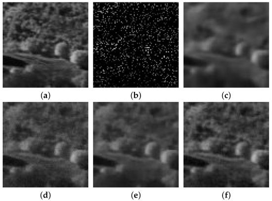
Figure 3. Results for CS reconstruction experiments in it Stanford (130th band). (a) original image, (b) observation, (c) ASTV, (d) SSTV, (e) HSSTV, (f) TNNG (ours)

4.2. Robust Principal Component Analysis

4.2.1. Image Decomposition

To evaluate our GRPCA, we first applied it to a standard sparse component decomposition. Following conventional methods such as [41], we randomly selected 30% of pixels in a HSI and replaced them with random values with a uniform distribution, which is a typical example to measure the performance of RPCA. The goal is to decompose the corrupted image to a latent low-rank HSI and the random values. We evaluated the performance with PSNR and SSIM between the corrupted image $\mathbf{y}$ and the obtained HSI $\mathbf{x}$ in (12) and compared it with the low-rank based decomposition methods, TRPCA [41] and LRTDTV [29].

We show the results in Table 2, where one can confirm that our method outperforms the conventional methods for most of the HSIs. This result shows that the proposed regularization function is able to correctly evaluate the image based on its low-rank nature. In addition, we believe that the proposed regularization function can evaluate the low-rank property of the image better than the conventional methods.

Table 2. Numerical results for image decomposition (PSNR [dB] / SSIM).

HSI	TRPCA	LRTDTV	GRPCA (ours)
PaviaC	35.16/0.961	38.17/0.966	40.45/0.977
PaviaU	35.01/0.965	36.93/0.964	39.55/0.976
Frisco	44.16/0.990	42.00/0.986	48.18/0.995
Stanford	41.80/0.980	44.05/0.986	48.19/0.993
Indian	35.43/0.940	37.06/0.961	37.87/0.988
Salinas	37.29/0.984	46.41/ 0.993	48.34/0.991
AVE. of 17 imgs	39.03/0.974	40.61/0.975	43.93/0.986

4.2.2. Mixed Anomaly Removal

We have tested the decomposition capability for images with mixed anomalies composed of dead lines/circles and impulsive noise. We compared our performance with TRPCA and LRTDTV. We conducted the removal of the anomaly pattern: sparsely scattered impulsive noise and dead lines/circles, where we prepare a mask for the dead lines and circles and generate images with dead pixels by multiplying the mask and an image (See Figure 4). We assume that anomalies sparsely appear, and then they can be removed in the low-rank component $\mathbf{x}$ in (12).

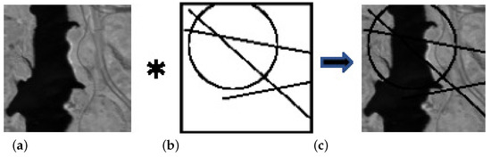
Figure 4. Dead lines/circles are generated by pixel-wise multiplication with mask. (a) original image, (b) mask, (c) generated image

We show our decomposition results in Figure 5 and the objective comparison in Table 3, where one can confirm that our method outperforms the conventional methods for most of the HSIs. Under mixed anomalies, we experimentally confirmed that TNNG maintains stable performance compared with the conventional methods, while the performance depends on experimental conditions and types of images in LRTDTV and TRPCA. This indicates that the image can be restored by using the spectral information of other pixels even if there is a defect in the gradient region due to the evaluation of low rankness.

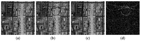
Figure 5. Results for GRPCA in Washington (76th band). (a) Input image, (b) Image with anomalies, (c) Low-rank component, (d) Sparse component

Table 3. Numerical results for mixed anomaly removal experiments: impulse (d = 10%) + dead lines/circles (PSNR [dB]/SSIM).

HSI	TRPCA	LRTDTV	GRPCA (ours)
PaviaC	37.95/ 0.981	41.22/0.977	42.25/0.981
PaviaU	37.73/0.982	40.4/0.976	41.45/0.983
Frisco	48.69/ 0.997	44.83/0.995	50.93/0.997
Stanford	45.79/0.994	50.33/ 0.997	50.95/0.995
Indian	37.25/0.969	37.58/ 0.970	38.88/0.970
Salinas	40.29/0.993	48.19/0.997	50.29/0.996
AVE. of 17 imgs	42.50/0.990	44.32/0.988	46.68/0.991

4.3. Pansharpening

We compared the proposed method defined by (14), with four conventional pansharpening methods: GFPCA [52], BayesNaive and BayesSparse [53], and HySure [54]. We conducted experiments on three types of noise levels, Type I (${\sigma }_{hs}=0.05,{\sigma }_{pan}=0.01$), Type II (${\sigma }_{hs}=0.1,{\sigma }_{pan}=0.01$), Type III (${\sigma }_{hs}=0.15,{\sigma }_{pan}=0.01$), where ${\sigma }_{hs}$ and ${\sigma }_{pan}$ are the standard deviation of noises added on a hyperspectral and a pan image, respectively.

Table 4 shows the comparison with the conventional methods. One can see from the results that our method outperforms the conventional methods in many cases. For subjective comparison, we show an example of the estimated HSIs from the data with Type I on PaviaC as shown in Figure 6.

Table 4. Numerical results for pansharpening: I (${\sigma }_{hs}=0.05,{\sigma }_{pan}=0.01$), II (${\sigma }_{hs}=0.1,{\sigma }_{pan}=0.01$), III (${\sigma }_{hs}=0.15,{\sigma }_{pan}=0.01$).

I
HSI		GFPCA	BayesNative	BayesSparse	HySure	TNNG (ours)
	PSNR	25.45	26.90	28.86	30.00	31.16
PaviaC	SAM	8.698	7.636	7.754	6.415	6.696
	ERGAS	6.396	5.668	4.625	3.808	3.368
	Q2n	0.248	0.337	0.339	0.473	0.484
	PSNR	24.85	26.51	27.67	29.26	30.25
PaviaU	SAM	9.346	7.718	8.568	7.176	7.001
	ERGAS	7.072	5.997	5.247	4.179	3.747
	Q2n	0.165	0.232	0.261	0.387	0.398
	PSNR	31.09	31.07	34.59	34.20	34.74
Frisco	SAM	3.973	5.451	3.733	4.338	4.594
	ERGAS	3.556	3.690	2.507	2.423	2.354
	Q2n	0.844	0.844	0.869	0.919	0.894
	PSNR	31.44	31.41	35.15	33.67	35.19
Stanford	SAM	4.398	7.614	4.204	3.822	5.928
	ERGAS	5.675	6.722	4.606	4.380	4.653
	Q2n	0.480	0.493	0.518	0.521	0.548
	PSNR	29.33	29.36	32.93	33.52	34.93
Suwannee	SAM	5.816	7.685	5.762	4.946	5.343
	ERGAS	3.717	3.917	2.556	2.341	2.214
	Q2n	0.516	0.560	0.597	0.612	0.662
II
	PSNR	25.37	25.55	28.53	29.45	29.76
PaviaC	SAM	9.159	11.888	8.481	7.238	8.964
	ERGAS	6.478	6.861	4.827	4.093	4.053
	Q2n	0.249	0.351	0.348	0.468	0.476
	PSNR	24.57	25.32	27.35	28.09	29.16
PaviaU	SAM	10.025	10.935	9.477	8.000	7.927
	ERGAS	6.974	6.269	5.188	4.542	4.069
	Q2n	0.167	0.198	0.275	0.347	0.348
	PSNR	30.82	28.83	33.82	32.86	33.48
Frisco	SAM	4.822	9.755	4.747	4.670	5.369
	ERGAS	3.719	5.106	2.804	2.940	2.876
	Q2n	0.843	0.844	0.874	0.892	0.893
	PSNR	31.10	29.06	34.33	32.98	33.89
Stanford	SAM	5.979	14.048	5.832	5.224	6.512
	ERGAS	6.437	11.421	5.567	5.343	4.958
	Q2n	0.478	0.497	0.519	0.516	0.516
	PSNR	29.13	27.38	32.30	32.29	33.48
Suwannee	SAM	6.696	12.619	6.895	5.389	6.098
	ERGAS	3.865	5.523	2.889	2.708	2.524
	Q2n	0.518	0.534	0.598	0.598	0.616
III
	PSNR	25.25	23.94	28.17	28.34	28.67
PaviaC	SAM	9.863	16.210	9.522	8.263	10.273
	ERGAS	6.611	8.596	5.126	4.680	4.542
	Q2n	0.256	0.313	0.376	0.419	0.433
	PSNR	24.65	23.99	27.23	27.79	28.81
PaviaU	SAM	10.225	14.694	9.848	8.940	8.503
	ERGAS	7.254	8.285	5.569	5.047	4.277
	Q2n	0.169	0.197	0.282	0.362	0.350
	PSNR	30.39	26.59	32.52	31.83	32.42
Frisco	SAM	6.000	14.050	6.105	6.951	6.440
	ERGAS	4.000	6.743	3.290	3.428	3.308
	Q2n	0.846	0.659	0.876	0.889	0.893
	PSNR	30.60	26.68	33.29	31.56	32.83
Stanford	SAM	7.927	20.437	7.926	7.312	7.823
	ERGAS	7.659	17.236	7.100	7.000	5.686
	Q2n	0.483	0.418	0.534	0.518	0.509
	PSNR	28.75	25.35	31.49	31.07	32.34
Suwannee	SAM	7.973	17.544	8.250	7.695	7.416
	ERGAS	4.160	7.376	3.327	3.378	2.924
	Q2n	0.514	0.407	0.603	0.593	0.592

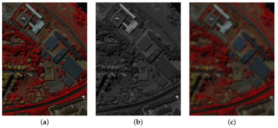
Figure 6. Data for Pansharpening in PaviaC ( Type I ). (a)original image, (b) pan image, (c) HSI.

The estimated HSIs with high spatial resolution are shown in Figure 7. Each PSNR[db] is 25.45 for (b), 26.90 for (c), 28.86 for (d), 30.0 for (e), and 31.16 for (f). We divided the band of these HSIs into three parts and visualized the average of each as RGB images. The details of the results obtained by GFPCA and BayesNaive are over-smoothed and its shading is unnatural. BayesSparse and HySure can estimate sharper images than those images, however, the texture of trees and buildings is lost. In contrast, the proposed method is particularly accurate in the restoration of the shading on the upper right and the texture of the central building on the upper left. As shown in (14), the optimization problem for pan-sharpening is the equation that minimizes the regularization function using the proposed method, and the number of hyperparameters is reduced by using constraints on HS and PAN images.

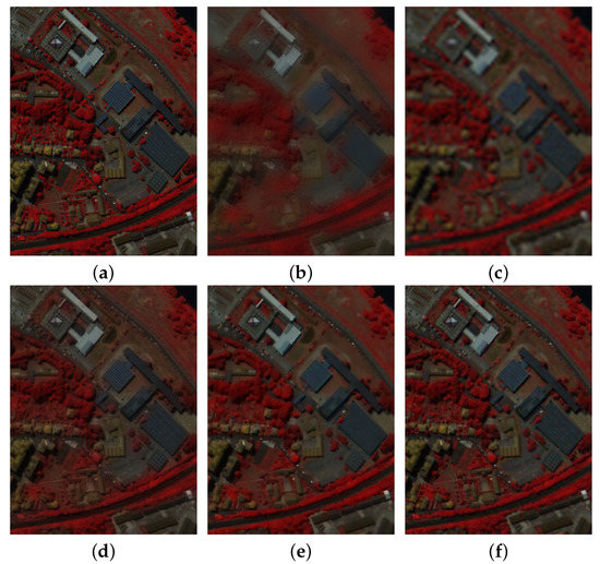
Figure 7. Results for Pansharpening experiments in PaviaC. (a) original image, (b) GFPCA, (c) BayesNaive, (d) BayesSparse, (e) HySure, (f) TNNG (ours).

5. Discussion

Computing Time

All methods are executed using Matlab 2019a on a MacBook Air (Retina, 13-inch, 2019), 1.6 GHz dual core Intel Core i5, and 16 GB 2133 MHz LPDDR3. The proposed method takes much more time than the conventional method. This is because the singular value decomposition of equation (7) needs to be performed $3n_v+3n_h$ times. Speeding up the processing is a major issue for the future, and we plan to pursue this point in the future.

• Compressed Sensing
  The maximum execution time for each method was about 2000 s for ASTV, 530 s for SSTV, 670 s for HSSTV, and 2500 s for TNNG (ours).
• Image Decomposition
  The maximum execution time for each method was about 1600 s for LRTDTV, 610 s for TRPCA, 2400 s for TNNG (ours).
• Mixed Anomaly Removal
  The maximum execution time for each method was about 1680 s for LRTDTV, 620 s for TRPCA, 2500 s for TNNG (ours).
• Pansharpening
  The maximum execution time for each method was about 4.2 s for GFPCA, 1.7 s for BayesNative, 130 s for BayesSparse, 110 s for HySure, and 7200 s for TNNG (ours).

6. Conclusions

In this paper, we proposed a new regularization scheme for HSI reconstruction called TNNG. We focused on the HSI property where the gradient image possesses strong inter-band correlation and utilized this property in the convex optimization. TNNG is a regularization scheme aimed at enforcing the low-rank gradient structure when observed from the spectral direction. We achieved high-performance HSI restoration by solving this regularized convex optimization problem using PDS. In experiments, we conducted compressed sensing reconstruction, image decomposition, and pansharpening. While the efficiencies of conventional methods depend on applications, the proposed method is superior to the conventional methods through both subjective and objective evaluations in various applications. In the proposed method, the process is done for a whole image without exploiting local features. It would be necessary for the future to consider further advances in performance by introducing local processing. And, the improvement of the calculation speed is also an issue.

References

- Ghamisi, P.; Yokoya, N.; Li, J.; Liao, W.; Liu, S.; Plaza, J.; Rasti, B.; Plaza, A. Advances in hyperspectral image and signal processing: A comprehensive overview of the state of the art. IEEE Geosci. Remote Sens. Mag. 2017, 5, 37–78. [Google Scholar] [CrossRef]
- Dian, R.; Li, S.; Fang, L.; Bioucas-Dias, J. Hyperspectral Image Super-Resolution via Local Low-Rank and Sparse Representations. In Proceedings of the IGARSS 2018-2018 IEEE International Geoscience and Remote Sensing Symposium, Valencia, Spain, 22–27 July 2018; pp. 4003–4006. [Google Scholar]
- Plaza, A.; Benediktsson, J.A.; Boardman, J.W.; Brazile, J.; Bruzzone, L.; Camps-Valls, G.; Chanussot, J.; Fauvel, M.; Gamba, P.; Gualtieri, A.; et al. Recent advances in techniques for hyperspectral image processing. Remote Sens. Environ. 2009, 113, S110–S122. [Google Scholar] [CrossRef]
- Bioucas-Dias, J.M.; Plaza, A.; Camps-Valls, G.; Scheunders, P.; Nasrabadi, N.; Chanussot, J. Hyperspectral Remote Sensing Data Analysis and Future Challenges. IEEE Geosci. Remote Sens. Mag. 2013, 1, 6–36. [Google Scholar] [CrossRef]
- Fu, Y.; Zheng, Y.; Sato, I.; Sato, Y. Exploiting spectral-spatial correlation for coded hyperspectral image restoration. In Proceedings of the IEEE Conference on Computer Vision and Pattern Recognition, Las Vegas, NV, USA, 27–30 June 2016; pp. 3727–3736. [Google Scholar]
- Khan, Z.; Shafait, F.; Mian, A. Joint group sparse PCA for compressed hyperspectral imaging. IEEE Trans. Image Process. 2015, 24, 4934–4942. [Google Scholar] [CrossRef]
- Shaw, G.; Manolakis, D. Signal processing for hyperspectral image exploitation. IEEE Signal Process. Mag. 2002, 19, 12–16. [Google Scholar] [CrossRef]
- Rizkinia, M.; Baba, T.; Shirai, K.; Okuda, M. Local spectral component decomposition for multi-channel image denoising. IEEE Trans. Image Process. 2016, 25, 3208–3218. [Google Scholar] [CrossRef]
- Jin, X.; Gu, Y. Superpixel-based intrinsic image decomposition of hyperspectral images. IEEE Trans. Geosci. Remote Sens 2017, 55, 4285–4295. [Google Scholar] [CrossRef]
- Zheng, Y.; Sato, I.; Sato, Y. Illumination and reflectance spectra separation of a hyperspectral image meets low-rank matrix factorization. In Proceedings of the IEEE Conference on Computer Vision and Pattern Recognition, Boston, MA, USA, 7–12 June 2015; pp. 1779–1787. [Google Scholar]
- Akhtar, N.; Shafait, F.; Mian, A. Futuristic greedy approach to sparse unmixing of hyperspectral data. IEEE Trans. Geosci. Remote Sens. 2015, 53, 2157–2174. [Google Scholar] [CrossRef]
- Bioucas-Dias, J.M.; Plaza, A.; Dobigeon, N.; Parente, M.; Du, Q.; Gader, P.; Chanussot, J. Hyperspectral Unmixing Overview: Geometrical, Statistical, and Sparse Regression-Based Approaches. IEEE J. Sel. Top. Appl. Earth Obs. Remote Sens. 2012, 5, 354–379. [Google Scholar] [CrossRef]
- Rizkinia, M.; Okuda, M. Joint Local Abundance Sparse Unmixing for Hyperspectral Images. Remote Sens. 2017, 9, 1224. [Google Scholar] [CrossRef]
- Liu, Y.; Condessa, F.; Bioucas-Dias, J.M.; Li, J.; Du, P.; Plaza, A. Convex Formulation for Multiband Image Classification with Superpixel-Based Spatial Regularization. IEEE Trans. Geosci. Remote Sens. 2018, 56, 2704–2721. [Google Scholar] [CrossRef]
- Zhang, H.; Li, J.; Huang, Y.; Zhang, L. A nonlocal weighted joint sparse representation classification method for hyperspectral imagery. IEEE J. Sel. Topics Appl. Earth Obs. Remote Sens. 2014, 7, 2056–2065. [Google Scholar] [CrossRef]
- Stein, D.W.J.; Beaven, S.G.; Hoff, L.E.; Winter, E.M.; Schaum, A.P.; Stocker, A.D. Anomaly detection from hyperspectral imagery. IEEE Signal Process. Mag. 2002, 19, 58–69. [Google Scholar] [CrossRef]
- Lefkimmiatis, S.; Roussos, A.; Maragos, P.; Unser, M. Structure tensor total variation. SIAM J. Imag. Sci. 2015, 8, 1090–1122. [Google Scholar] [CrossRef]
- Ono, S.; Shirai, K.; Okuda, M. Vectorial total variation based on arranged structure tensor for multichannel image restoration. In Proceedings of the 2016 IEEE International Conference on Acoustics, Speech and Signal Processing (ICASSP), Shanghai, China, 20–25 March 2016; pp. 4528–4532. [Google Scholar]
- Prasath, V.B.S.; Vorotnikov, D.; Pelapur, R.; Jose, S.; Seetharaman, G.; Palaniappan, K. Multiscale Tikhonov-total variation image restoration using spatially varying edge coherence exponent. IEEE Trans. Image Process. 2015, 24, 5220–5235. [Google Scholar] [CrossRef] [PubMed]
- Zhang, H. Hyperspectral image denoising with cubic total variation model. ISPRS Ann. Photogramm. Remote Sens. Spat. Inf. Sci. 2012, I-7, 95–98. [Google Scholar] [CrossRef]
- Yuan, Q.; Zhang, L.; Shen, H. Hyperspectral image denoising employing a spectral-spatial adaptive total variation model. IEEE Trans. Geosci. Remote Sens. 2012, 50, 3660–3677. [Google Scholar] [CrossRef]
- He, W.; Zhang, H.; Zhang, L.; Shen, H. Total-variation-regularized low-rank matrix factorization for hyperspectral image restoration. IEEE Trans. Geosci. Remote Sens. 2016, 54, 178–188. [Google Scholar] [CrossRef]
- Zhang, H.; He, W.; Zhang, L.; Shen, H.; Yuan, Q. Hyperspectral image restoration using low-rank matrix recovery. IEEE Trans. Geosci. Remote Sens. 2014, 52, 4729–4743. [Google Scholar] [CrossRef]
- Sun, L.; He, C.; Zheng, Y.; Tang, S. SLRL4D: Joint Restoration of Subspace Low-Rank Learning and Non-Local 4-D Transform Filtering for Hyperspectral Image. Remote Sens. 2020, 12, 2979. [Google Scholar] [CrossRef]
- Condat, L. A primal-dual splitting method for convex optimization involving Lipschitzian, proximable and linear composite terms. J. Optim. Theory Appl. 2013, 158, 460–479. [Google Scholar] [CrossRef]
- Dabov, K.; Foi, A.; Egiazarian, K. Video denoising by sparse 3D transform-domain collaborative filtering. In Proceedings of the European Signal Processing Conference, Poznan, Poland, 3–7 September 2007. [Google Scholar]
- Aggarwal, H.K.; Majumdar, A. Hyperspectral image denoising using spatio-spectral total variation. IEEE Geosci. Remote Sens. Lett. 2016, 13, 442–446. [Google Scholar] [CrossRef]
- Takeyama, S.; Ono, S.; Kumazawa, I. Hyperspectral image restoration by hybrid spatio-spectral total variation. In Proceedings of the 2017 IEEE International Conference on Acoustics, Speech and Signal Processing, New Orleans, LA, USA, 5–9 March 2017; pp. 4586–4590. [Google Scholar]
- Wang, Y.; Peng, J.; Zhao, Q.; Leung, Y.; Zhao, X.L.; Meng, D. Hyperspectral image restoration via total variation regularized low-rank tensor decomposition. IEEE J. Sel. Top. Appl. Earth Obs. Remote Sens. 2018, 11, 1227–1243. [Google Scholar] [CrossRef]
- Lim, B.; Son, S.; Kim, H.; Nah, S.; Lee, K.M. Enhanced deep residual networks for single image super-resolution. In Proceedings of the IEEE Conference on Computer Vision and Pattern Recognition (CVPR) Workshops, Honolulu, HI, USA, 21–26 July 2017; Volume 1, p. 4. [Google Scholar]
- Park, D.; Kim, K.; Chun, S.Y. Efficient module based single image super resolution for multiple problems. In Proceedings of the IEEE Conference on Computer Vision and Pattern Recognition (CVPR) Workshops, Salt Lake City, UT, USA, 18–22 June 2018; Volume 5. [Google Scholar]
- Nie, S.; Gu, L.; Zheng, Y.; Lam, A.; Ono, N.; Sato, I. Deeply Learned Filter Response Functions for Hyperspectral Reconstruction. In Proceedings of the IEEE Conference on Computer Vision and Pattern Recognition, Salt Lake City, UT, USA, 18–22 June 2018; pp. 4767–4776. [Google Scholar]
- Qu, Y.; Qi, H.; Kwan, C. Unsupervised Sparse Dirichlet-Net for Hyperspectral Image Super-Resolution. In Proceedings of the IEEE Conference on Computer Vision and Pattern Recognition, Salt Lake City, UT, USA, 18–22 June 2018; pp. 2511–2520. [Google Scholar]
- Shi, Z.; Chen, C.; Xiong, Z.; Liu, D.; Wu, F. Hscnn+: Advanced cnn-based hyperspectral recovery from rgb images. In Proceedings of the IEEE/CVF Conference on Computer Vision and Pattern Recognition Workshops (CVPRW), Salt Lake City, UT, USA, 18–22 June 2018; Volume 3, p. 5. [Google Scholar]
- Matsuoka, R.; Ono, S.; Okuda, M. Transformed-domain robust multiple-exposure blending with Huber loss. IEEE Access 2019, 7, 162282–162296. [Google Scholar] [CrossRef]
- Imamura, R.; Itasaka, T.; Okuda, M. Zero-Shot Hyperspectral Image Denoising with Separable Image Prior. In Proceedings of the IEEE International Conference on Computer Vision Workshops, Seoul, Korea, 27–28 October 2019. [Google Scholar]
- Baraniuk, R.G. Compressive sensing. IEEE Signal Process. Mag. 2007, 24, 118–121. [Google Scholar] [CrossRef]
- Candès, E.; Wakin, M. An introduction to compressive sampling. IEEE Signal Process. Mag. 2008, 25, 21–30. [Google Scholar] [CrossRef]
- Candès, E.J.; Li, X.; Ma, Y.; Wright, J. Robust principal component analysis? J. ACM (JACM) 2011, 58, 11. [Google Scholar] [CrossRef]
- Lu, C.; Feng, J.; Chen, Y.; Liu, W.; Lin, Z.; Yan, S. Tensor robust principal component analysis: Exact recovery of corrupted low-rank tensors via convex optimization. In Proceedings of the IEEE Conference on Computer Vision and Pattern Recognition, Las Vegas, NV, USA, 27–30 June 2016; pp. 5249–5257. [Google Scholar]
- Lu, C.; Feng, J.; Chen, Y.; Liu, W.; Lin, Z.; Yan, S. Tensor Robust Principal Component Analysis with A New Tensor Nuclear Norm. arXiv 2018, arXiv:1804.03728. [Google Scholar] [CrossRef] [PubMed]
- Combettes, P.L.; Pesquet, J.C. Proximal Splitting Methods in Signal Processing; Springer: Berlin/Heidelberg, Germany, 2011; pp. 185–212. [Google Scholar]
- Moreau, J.J. Fonctions convexes duales et points proximaux dans un espace hilbertien. C. R. Acad. Sci. Paris Ser. A Math. 1962, 255, 2897–2899. [Google Scholar]
- Chambolle, A.; Pock, T. A first-order primal-dual algorithm for convex problems with applications to imaging. J. Math. Imag. Vis. 2010, 40, 120–145. [Google Scholar] [CrossRef]
- Combettes, P.L.; Pesquet, J.C. Primal-dual splitting algorithm for solving inclusions with mixtures of composite, Lipschitzian, and parallel-sum type monotone operators. Set Valued Variation. Anal. 2012, 20, 307–330. [Google Scholar] [CrossRef]
- Wang, Z.; Bovik, A.C.; Sheikh, H.R.; Simoncelli, E.P. Image quality assessment: From error visibility to structural similarity. IEEE Trans. Image Process. 2004, 13, 600–612. [Google Scholar] [CrossRef] [PubMed]
- Kruse, F.; Lefkoff, A.; Boardman, J.; Heidebrecht, K.; Shapiro, A.; Barloon, P.; Goetz, A. The spectral image processing system (SIPS)—interactive visualization and analysis of imaging spectrometer data. Remote Sens. Environ. 1993, 44, 145–163. [Google Scholar] [CrossRef]
- Wald, L. Quality of high resolution synthesised images: Is there a simple criterion? In Third Conference “Fusion of Earth Data: Merging Point Measurements, Raster Maps and Remotely Sensed Images”; Ranchin, T., Wald, L., Eds.; SEE/URISCA: Sophia Antipolis, France, 2000; pp. 99–103. [Google Scholar]
- Garzelli, A.; Nencini, F. Hypercomplex Quality Assessment of Multi/Hyperspectral Images. IEEE Geosci. Remote Sens. Lett. 2009, 6, 662–665. [Google Scholar] [CrossRef]
- Hyperspectral Remote Sensing Scenes. Available online: http://www.ehu.eus/ccwintco/index.php (accessed on 20 October 2017).
- Skauli, T.; Farrell, J. A collection of hyperspectral images for imaging systems research. In Proceedings of the SPIE Electronic Imaging, San Francisco, CA, USA, 3–7 February 2013. [Google Scholar]
- Liao, W.; Huang, X.; Van Coillie, F.; Gautama, S.; Pizurica, A.; Philips, W.; Liu, H.; Zhu, T.; Shimoni, M.; Moser, G.; et al. Processing of Multiresolution Thermal Hyperspectral and Digital Color Data: Outcome of the 2014 IEEE GRSS Data Fusion Contest. IEEE J. Sel. Top. Appl. Earth Obs. Remote Sens. 2015, 8, 2984–2996. [Google Scholar] [CrossRef]
- Wei, Q.; Dobigeon, N.; Tourneret, J. Bayesian Fusion of Multi-Band Images. IEEE J. Sel. Top. Signal Process. 2015, 9, 1117–1127. [Google Scholar] [CrossRef]
- Simoes, M.; Bioucas-Dias, J.; Almeida, L.B.; Chanussot, J. A Convex Formulation for Hyperspectral Image Superresolution via Subspace-Based Regularization. IEEE Trans. Geosci. Remote Sens. 2015, 53, 3373–3388. [Google Scholar] [CrossRef]
Publisher’s Note: MDPI stays neutral with regard to jurisdictional claims in published maps and institutional affiliations. |
© 2021 by the authors. Licensee MDPI, Basel, Switzerland. This article is an open access article distributed under the terms and conditions of the Creative Commons Attribution (CC BY) license (http://creativecommons.org/licenses/by/4.0/).