Abstract
The World Health Organization has reported that the number of worldwide urban residents is expected to reach 70% of the total world population by 2050. In the face of challenges brought about by the demographic transition, there is an urgent need to improve the accuracy of urban land-use mappings to more efficiently inform about urban planning processes. Decision-makers rely on accurate urban mappings to properly assess current plans and to develop new ones. This study investigates the effects of including conventional spectral signatures acquired by different sensors on the classification of airborne LiDAR (Light Detection and Ranging) point clouds using multiple feature spaces. The proposed method applied three machine learning algorithms—ML (Maximum Likelihood), SVM (Support Vector Machines), and MLP (Multilayer Perceptron Neural Network)—to classify LiDAR point clouds of a residential urban area after being geo-registered to aerial photos. The overall classification accuracy passed 97%, with height as the only geometric feature in the classifying space. Misclassifications occurred among different classes due to independent acquisition of aerial and LiDAR data as well as shadow and orthorectification problems from aerial images. Nevertheless, the outcomes are promising as they surpassed those achieved with large geometric feature spaces and are encouraging since the approach is computationally reasonable and integrates radiometric properties from affordable sensors.
1. Introduction
The world urban population began to increase significantly since the 1950s. In 1980, around 40% of the total world population lived in cities. This percentage increased to 50% in 2010. In the near future, the growth rate of the urban population is expected to be approximately 1.63% and 1.44% per year between 2020 and 2025 and between 2025 and 2030, respectively. Moreover, by 2050, the urban population is expected to almost double, increasing from approximately 3.4 billion (American billion = 10) in 2009 to 6.4 billion [1]. This tangible demographic transition has environmental impacts, such as the loss of agricultural lands, reduction in wildlife habitats, air pollution, and a worsening of water quality and accessibility, leading to a deterioration of regional hydrology. Furthermore, urbanization has a significant side effect of exacerbating the already uneven allocation of resources in urban areas. Resource disparity is a well-known progenitor of a plethora of societal issues, including scarcity of affordable housing, poverty, constrained social services, and an increased crime rate [2,3]. To bridge the gap between the available resources and the needs of an urban population, a thorough urban land-use classification becomes an urgent necessity for further urban assessment, and future city planning and management [1].
High-resolution optical images provide a high level of detail along object boundaries with height variations. Therefore, they are a good source of high horizontal-accuracy data and a rich inventory of spectral and textural information essential for segmentation and classification [4]. However, these conventional sensors lack vertical accuracy due to their inability to fully represent spatial patterns in 3D [5]. In some cases, they acquire information from a relatively restricted number of bands, each with large spectral intervals. Consequently, they are not suitable for detailed analysis of classes sharing similar characteristics in contrast to the new generation of passive hyperspectral sensors [6]. On the other hand, LiDAR (Light Detection and Ranging) systems acquire high-density 3D point clouds about the shape of the Earth and its surface characteristics. The penetration capability of the laser pulses reveals certain ground objects in a single pulse with multiple returns. Hence, they can effectively cover large regions and can collect data in steep terrains with no shadow effects or occlusion if sufficient swath overlap can be achieved. Moreover, all obtained data are directly geo-referenced [7,8,9]. Nevertheless, since the discontinuous laser pulses can hardly hit breaklines, LiDAR technologies show poor performance in revealing surfaces with sudden elevation changes. Thus, they produce insufficient 3D point clouds at these positions, weakening the horizontal accuracy of such locations [10].
Given the complementary properties of LiDAR and optical data imaging, integrating the two modalities in the information extraction procedure becomes attractive as a means to amplify their strengths and to overcome their respective weaknesses. Such a fusion provides a practical alternative to the more expensive multispectral/hyperspectral LiDAR systems. The case for integrating these two modalities is especially compelling in applications that require high-density acquisitions for large regions [11,12]. In particular, the high cost associated with flights and radiometric corrections makes integrating LiDAR and optical data an excellent candidate when dealing with data obtained from airborne platforms [11].
This integration opens the door to mapping LULCs (Land Use Land Cover) other than urban settings. For example, LULCs can be used in agricultural and forestry morphologies to observe crop biomass and to estimate their production and environmental states. Such applications have recently turned to relying on acquiring aerial images and LiDAR point clouds using sensors mounted on UAVs (Unmanned Aerial Vehicle); therefore, combining both data types reinforces the textual analysis of agricultural fields [13]. In addition, infrastructural inspection and structural health-monitoring applications depend on information extracted from thermal images and LiDAR scans collected by UASs (Unmanned Aircraft System) for precise close-range inspection and trajectory control [14]. These utilizations are added to retrofitting applications that align 3D laser scans with camera videos for complex industrial modeling such as those in pipeline plants [15]; aerial cinematography that utilizes dynamic camera viewpoints for entertainment, sports, and security applications [16]; and synchronized human–robot interaction applications such as the prediction of pedestrian attitude on roads for potential urban automated driving [17].
Classification is the process of partitioning data into a finite number of individual categories based on the attributes stored in each data element. The purpose of classification is to identify homogeneous groups representing various urban classes of interest [18]. The classification results are fundamental in further analysis for many environmental and socioeconomic applications, such as in change detection and simulation/prediction models. Therefore, a classification system should be informative, exhaustive, separable, and homogeneous with a range of variability of each respective class. The classification process itself requires consideration of different factors. These factors include the needs of the end-user, the scale of the area studied, the complexity of the landscape within it, and the nature of the data being processed [19,20]. Machine learning is an AI (Artificial Intelligence) application that enables computers to learn automatically with minimal human assistance. Machine learning algorithms identify patterns in observations to make predictions or to improve existing predictions when trained on similar data [21]. Machine learning approaches can be grouped into different categories: supervised, unsupervised, semi-supervised, and reinforcement based on the learning type; parametric versus nonparametric based on the assumption of the data distribution; hard versus soft/fuzzy based on the number of outputs for each spatial unit; and finally, pixel-based, object-based, and point-based classifications based on the nature of data at hand [19,21].
In supervised learning, analysts must select representative samples for each category for the classifier to determine the classes for each element of the entire dataset [22]. In contrast, unsupervised classification does not require any prior class knowledge of the study region. Instead, concentrations of data with similar features (clusters) are detected within a possibly heterogeneous dataset. Unsupervised learning could be advantageous to supervised learning in cases where prior class knowledge is incomplete. However, the resulting data clusters from unsupervised learning do not necessarily align with the class classification criteria as prescribed by the problem being investigated [23,24]. Semi-supervised learning falls in between supervised and unsupervised learning since it uses both labeled and unlabeled training data. It has become a hot topic in classifying remotely sensed data that contain large sets of unlabeled examples with very few labeled ones. Its algorithms are extensions of other approaches that make assumptions about modeling unlabeled data [21,25]. Reinforcement learning follows a trial-and-error search for the ideal behavior to boost its performance. The best action is detected by simple reward feedback known as the reinforcement signal [21]. Parametric approaches assume the existence of an underlying data probability distribution (usually the normal distribution). The parameters of this underlying distribution (i.e., mean vector and covariance matrix) have to be estimated from the training samples to trigger the classification process. Nonparametric algorithms make no assumptions about the form of the data probability distribution. They have been proven to perform efficiently with various class distributions as long as their signatures are adequately distinct. Moreover, nonparametric methods allow for ancillary data incorporation into the classification procedure in contrast to parametric algorithms that are more susceptible to noise while dealing with complex landscapes and often present challenges in incorporating non-remote-sensing data within classification [22,24,26].
Each data element in hard thematic maps is assigned to a single class. Hard classifiers sometimes cause misclassification errors, especially when using coarse spatial resolution data with multi-class representation. In contrast, soft classifiers determine a range of data similarity to all classes. Consequently, each data element is assigned to every class with varying probabilities, resulting in a more informative and potentially more accurate classification. However, soft classification lacks spatial information about each class within each data element [26,27]. In pixel-based classification, the classifier gathers spectra of every pixel used in the training samples to develop a signature of each class [26] while simultaneously assigning a single predefined category to each pixel based on the brightness value the pixel stores [23]. Meanwhile, object-based approaches generate fundamental units of image classification from object segmentation at various scale levels based on specific homogeneity criteria instead of raster data elements: a single pixel [23,28]. Pixel-based techniques best fit coarse data, while object-based approaches perform well in matching data acquired at fine spatial resolutions. Point-based classifiers are commonly used to process LiDAR point clouds. These point-based classifiers are similar to pixel-based techniques in terms of dealing with each single data element—a single point—individually and assign a particular predefined class for each of those points [23].
Brownlee [25] added another classification of machine learning algorithms based on similarity and functionality. Here is a summary of their taxonomy:
- Regression algorithms model the relationship between variables and refine it iteratively by adjusting prediction errors (i.e., linear and logistic regression).
- Instance-based algorithms use observations to construct a database, to which new data are compared to find the best match for prediction using a similarity measure (i.e., KNN (K-Nearest Neighbors) and SVM (Support Vector Machine)).
- Regularization algorithms extend regression methods to prioritize simple models over complex ones for better generalization (i.e., ridge and least-angle regression).
- Decision tree algorithms build a model of decisions based on the observations’ attribute values. These decisions branch until a prediction is made for a certain record (i.e., decision tump and conditional decision trees).
- Bayesian algorithms apply Bayes’ Theorem (i.e., naive Bayes and Gaussian naive Bayes).
- Clustering algorithms use built-in data structures to produce groups of maximum commonality (i.e., k-means and k-medians).
- Association rule learning algorithms derive formulas that best explain the relationships between the variables of observations. These rules are generic enough to be applied to large multidimensional datasets (i.e., apriori and eclat).
- Artificial neural network algorithms are pattern-matching-based methods inspired by biological neural networks (i.e., perceptron and MLP (Multilayer Perceptron Neural Network)).
- Deep learning algorithms are higher levels of artificial neural networks (i.e., convolutional and recurrent neural networks).
- Dimensionality reduction algorithms reduce data dimensionality in an unsupervised approach for better space visualization. Abstracted dimensions can be input into a subsequent supervised algorithm (i.e., PCA (Principal Component Analysis) and PCR (Principal Component Regression)).
- Ensemble algorithms are strong learners consisting of multiple weaker learners that are independently trained in parallel and vote toward the final prediction of a record (i.e., Bagging, AdaBoost, and RF (Random Forest)).
Most initial studies that addressed LiDAR data classification tended to convert point clouds into 2D images [29] by applying interpolation techniques, which vary in complexity, ease of use, and computational expense; and thus, no interpolation method is universally superior [30]. Interpolation methods are either deterministic (i.e., IDW (Inverse Distance Weighted) and spline), or probabilistic (i.e., Kriging). Deterministic algorithms calculate the value of an unsampled point given the known data values of its immediate surrounding sampled points. A predetermined mathematical formula calculates the weight of each surrounding point contributing to the interpolated result. The calculations end up with a continuous spatial surface. Probabilistic algorithms utilize spatial autocorrelation properties (i.e., distance and direction) of the surrounding values to determine their importance [30,31]. Cell size determination is the primary concern in generating LiDAR images via interpolation techniques. Therefore, resolutions have to ensure the acquisition of sufficient details but also with the least amount of point data that meets the minimum accuracy assigned for the phenomenon being studied. Too fine-resolutions are overrepresentative and computationally ineffective. Hence, an optimal grid size should consider data source density, terrain complexity, and nature of the application [31]. For instance, DEM accuracy is affected by spatial resolution along with interpolation error and algorithm, which have to be taken into consideration, since low DEM accuracy accordingly impacts the accuracy of its derived terrain attributes, such as slope [30,32].
The LiDAR capabilities of recording different point attributes (i.e., intensity, elevation, range, and number of returns) have encouraged analysts to resample point clouds into 2D grids based on a predefined resolution. In doing so, analysts gain performance advantages in computations at the expense of sacrificing details representing data in 2D instead of 3D [23,29]. These missing details can be vital in some applications, mostly when oriented toward objects that are not easily separable from other features. For example, in evaluating the solar potential of roof planes, downsampling and interpolation adversely affect the estimation of their aspect, inclination angles, and areas. These defects significantly impact the assessment results [33]. Figure 1 graphically illustrates how certain information is lost in resampling irregularly spaced classified points to a grid in order to produce a LULC map [23]. The authors identified the extent of the study area (Figure 1a) and constructed a grid, where each cell was assigned the same size as the laser beam footprint (Figure 1b). Then, the resampled point of each cell had the most frequent class of classified points within the cell itself (Figure 1c). Empty cells were assigned an unclassified grid point and were treated as gaps that were to be filled by NN (Nearest Neighbor) and IMMW (Iterative Majority Moving Window). In NN, unclassified resampled points were assigned to the class of the nearest original classified LiDAR point. In IMMW, a moving window was centered at each of the unclassified resampled points. They were assigned to the most frequent class of their neighbors iteratively until all gaps were filled. The study indicated no difference between both filling approaches, as the overall classification accuracies using ML (Maximum Likelihood) did not exceed 58% using the points’ elevation and intensity. In another study, the same classification workflow was examined against the pixel-based classification of LiDAR images of two different datasets [34]. It yielded overall map accuracies of 44% and 50% with the pixel-based classification and of 53% and 65% with the point-based approach, respectively, for each dataset. The higher achieved map accuracy was highlighted with LiDAR raw data points classification, as it was carried out based on the original data values.
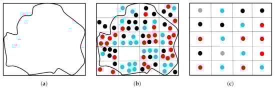
Figure 1.
Resampling of classified points: turquoise, black, and red represent points of three different classes, and grey points represent unclassified resampled points. (a) Extent of study area. (b) Pixel-size identification. (c) Point resampling into the grid.
Lodha et al. [35] resampled 3D LiDAR data into a regular 2D grid, which they geo-registered to a grey-scale aerial image of the same grid size. After fusing the height and intensity data, they generated a 5D feature space of height, height variation, normal variation, LiDAR intensity, and image intensity. The feature space was subsequently used to classify an urban layout into roads, grass, buildings, and trees, using the AdaBoost algorithm. Since AdaBoost was originally a binary classifier, the study applied the AdaBoost.M2 extension for multiclass categorization and achieved an accuracy of around 92%. Gao and Li [36] applied the AdaBoost algorithm but followed a direct point-based classification on 3D LiDAR clouds, with only height and intensity included in the feature space. When tested on different LiDAR datasets, the highest accuracy of this scenario was close to what was achieved in [35].
Wang et al. [37] also rasterized airborne LiDAR point clouds into grids for data based on height information; however, they constructed the feature space differently. They randomly selected two neighboring pixels of each pixel from a moving window with a predefined size. Afterward, they calculated the height difference between the two pixels. To enlarge the dimension of the feature space, they repeated the random selection. With each new selection, a different feature was compared in addition to the height value. Therefore, for each pixel, the total number of random selections of neighboring pixels was the number of features used in the classification. The study applied RF to classify the urban scene into ground, buildings, cars, and trees. It resulted in an overall map accuracy of 87% after postprocessing using majority analysis and identified major problems distinguishing cars and trees from the ground.
In an attempt to enrich the feature space for better point-based classification results, Zaboli et al. [38] considered eigenvalues, geometric, and spatial descriptors along with intensity records in the discrete point classification of mobile terrestrial LiDAR data. These contextual features were computed for each point within a neighborhood to explore further information about spatial dependency. The study compared the GNB (Gaussian Naive Bayes), KNN, SVM, MLP, and RF’s potential capabilities to classify an urban scene containing cars, trees, poles, powerlines, asphalt roads, sidewalks, buildings, and billboards. The maximum overall accuracy was 90% by RF in contrast to an accuracy of 53% achieved by GNB. Niemeyer et al. [39] also used waveform and geometry descriptors but with a hierarchical classifier in the point-based classification of airborne LiDAR data covering roads, soil, low vegetation, trees, buildings, and cars. The study implemented a two-layer CRF (Conditional Random Field), where a point-based classification runs in the first layer and a segment-based classification is performed in the second one. RF was applied in both classifications. Each segment’s probability of belonging to a certain class was generated in the second layer and delivered to the first layer at each iteration via a cost term. In this way, regional context information between segments was transferred to the point layer, where misclassification was eliminated. Although this approach increased the overall accuracy by 2% on a point-based level, it still hovered around 80%.
Researchers have recently investigated multispectral LiDAR data as a promising option towards widening the radiometric feature space. Huo et al. [40] constructed their feature space by converting the three intensities of Optech Titan LiDAR point clouds into images. Furthermore, they densified the space with some auxiliary features: NDSM (Normalized Digital Surface Model), pseudo NDVI (Normalized Difference Vegetation Index), MP (Morophological Profile), and HMP (Hierarchical Morophological Profile). The study applied SVM to classify buildings, grass, roads, and trees. The authors tried different combinations of feature sets and concluded that using only intensity features resulted in the worst overall map accuracy, i.e., 75%, while the addition of the remaining features was the best scenario, which achieved a 93% accuracy.
On the other hand, Morsy et al. [41] processed 3D point clouds acquired by a multispectral LiDAR sensor, which covered an urban scene consisting of four classes: buildings, trees, roads, and grass. The data were ground filtered. Jenks natural breaks optimization method clustered the points into the four predefined classes based on three NDVIs calculated for each point using its intensity of the three channels: NIR (Near Infrared), MIR (Mid Infrared), and Green. The clustering algorithm determined NDVI thresholds to segregate buildings from trees and roads from grasses. It relies on the fact that vegetation has higher reflectance in the abovementioned channels than built-up elements. A subset of the LiDAR point clouds from each class was selected by a set of polygons, as reference points, and together with a geo-referenced aerial image were used to assess the classification accuracy. The results showed that the NDVI produced from the NIR and Green channels had the highest overall accuracy, i.e., 92.7%. Alternatively, the authors adopted the Gaussian decomposition clustering approach for the determination of NDVI thresholds [42]. They used the peak detection algorithm to find the highest two peaks of the NDVI histograms. These peaks were considered the mean of each Gaussian component of the histogram, which had two components, as the target was to divide each histogram into two clusters: either buildings and trees or roads and grass. The component’s mean, standard deviation, and relative weight were fitted on two steps: expectation and maximization. The first determined the probability of each bin belonging to either Gaussian components, starting with the assumption that both components have the same weight, and the latter computed the ML estimates of the component’s statistics. Both steps were repeated until either a convergence or a maximum number of trials was reached. The intersection of both fitted components was considered a threshold. The algorithm resulted in an overall accuracy of 95.1%, with the same NDVI as in the Jenks natural breaks optimization clustering method. Despite the higher accuracy achieved without auxiliary data (i.e., NDSM), the study reported overfitting problems, which forced the authors to apply different modeling functions, sacrificing precise definition of the threshold value and consequently affecting the accuracy of some classes.
Imagery data represent a rich source of radiometric characteristics, other than multispectral LiDAR sensors. Several studies have introduced aerial and high-resolution satellite images as an ancillary data source in LiDAR point clouds classification. They were even a substantial source of 3D point clouds utilized in some research materials. Baker et al. [43] processed aerial photogrammetric images to obtain their respective dense point clouds, which were classified using the RF and GBT (Gradient Boosted Trees) classifiers to detect buildings, terrain, high vegetation, roads, cars, and other human-made objects. Pearson product–moment correlation coefficient and the Fisher information were processed on the training samples. Both metrics indicated that HSV (Hue Saturation Value) was the most informative portion of the color space used in color feature extraction. Different combinations of features and classifiers were run and evaluated, revealing a significant increase in the overall classification accuracy when color features were combined and in the GBT classifier’s superiority versus RF. Zhou et al. [44] considered DIM (Dense Image Matching) point clouds as auxiliary data to classify airborne LiDAR clouds on a point-based level within a novel framework. For DIM and LiDAR point clouds, they built a 13D feature space that included purely geometric descriptors: height, eigenvalue, normal vector, curvature, and roughness features. Then, they extracted useful samples from DIM points as training data using the extended multi-class TrAdaboost and input the features of all DIM and LiDAR point clouds to a weighted RF model. In the following iteration, DIM misclassified samples were assigned lesser weights. Consequently, poor DIM sample points were eliminated and useful ones were retained. The authors tested the method on different urban scenes with buildings, ground, and vegetation. The best overall accuracy they obtained was 87%. However, their approach saves computational time since it does not require DIM-LiDAR registration. Moreover, DIM points can be acquired for different scenes, as long as they capture similar classes.
This literature review concludes that the classification of LiDAR data on a point-based level is more accurate than pixel-based classification since spatial and spectral information are partially lost in the latter. Moreover, it highlights the importance of expanding the feature space dimensions to include more descriptors for better mapping results. Most importantly, the referenced experimental work indicates the effectiveness of considering a slim set of color features over a large number of geometric descriptors in enhancing the classification results. The overall accuracy did not exceed 90% in the vast majority of the mentioned studies, which focused on computing high-dimensional geometric-oriented feature space. On the other hand, the mapping accuracy barley passed 95% in [42], only with the addition of the NDVI features derived from a multispectral LiDAR sensor. Therefore, we focus in this paper on fusing spectral descriptors inherited from more affordable sensors in the point-based classification of airborne LiDAR clouds. In particular, we explore the effect of the gradual inclusion of the red, green, blue, NIR, and NDVI features integrated from corresponding aerial photos, on the accuracy results using the ML, SVM, MLP, and Bagging supervised classifiers. The presented work gives thorough insights on each scenario in terms of training and validation data size and distribution, learning behavior, processing time, and per-class accuracy for each classifier.
The remaining body of the paper presents the following sections: Methods, Experimental Work, Results, Discussion, and Conclusions.
2. Methods
The proposed workflow is illustrated in Figure 2. LiDAR point clouds were first geo-registered to an aerial photo of the same scene so that each point inherited its corresponding spectral properties. In addition, spectral indices could also be derived (i.e., NDVI). The point clouds were then filtered to separate those belonging to the ground from non-ground points. Afterward, training samples were acquired to serve three classifiers: ML, SVM, and MLP with multiple feature combinations (scenarios). The classification results were assessed to target the most accurate and precise scenario for a subsequent classification using the Bagging and Voting ensemble algorithms, respectively. The final land-use map was evaluated to ensure its quality in general and in comparison with the maps derived from the same feature combination by each of the three classifiers.
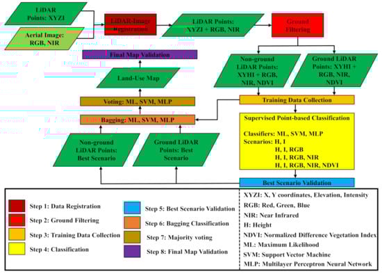
Figure 2.
Conceptual overview of the proposed methodology.
2.1. LiDAR-Image Geo-Registration
The LiDAR point clouds were geo-registered to an aerial image of the same study region in [45] to inherit additional spectral properties. The geo-registration approach was applied the PC (Phase Congruency) model and a scene abstraction approach to detect edge points in both aerial and LiDAR images. These edge points act as candidate control points, which were matched as final control points using the shape context descriptor. The registration parameters of the polynomial models were estimated using a least-squares optimization method. The semi-automatic approach was found to overcome the issue of identifying interrelated control points between LiDAR and imagery data that were obtained at different times. This coping came from clustering both images based on their edge potentiality and the target points on mutual outlines as control points. In this way, registration primitives are no longer limited to traditional linear urban elements. Moreover, the phase congruency model runs on lower spatial-resolution versions of the images, which speeds up the processing and contributes more to figuring out common control points in both images. A detailed description of the geo-registration process can be found in [46].
2.2. LiDAR Ground Filtering
Discriminating terrain points from non-terrain points is a fundamental step in LiDAR classification applications, where ground objects share characteristics with non-ground features. In this case, ground filtering helps minimize misclassification errors. Zhang and Lin [47] grouped ground filtering techniques into four main categories according to directional scanning, ground definition, filtering concept, and means of creating the surface (Figure 3). Directional scanning techniques are sub-grouped into directional-based and neighborhood-based approaches. Directional-based approaches separate terrain from non-terrain points by calculating elevation or slope differences along a 1D scan line in a certain direction [48]. Neighborhood-based algorithms consider the values of the surrounding points within a predefined neighborhood [49]. According to the ground definition, a ground filtering technique can be either a labeling or an adjustment approach. An adjustment approach applies a mathematical function to LiDAR point clouds, where points within a threshold of vertical distances from the Earth’s surface are considered ground points. A least-squares adjustment detects non-ground points as blunders and reduces their weights in each iteration. Labeling approaches are different, as they use certain operators (i.e., morphology and slope) to distinguish ground points from non-ground points [50]. These operators were addressed in the filtering categories below.
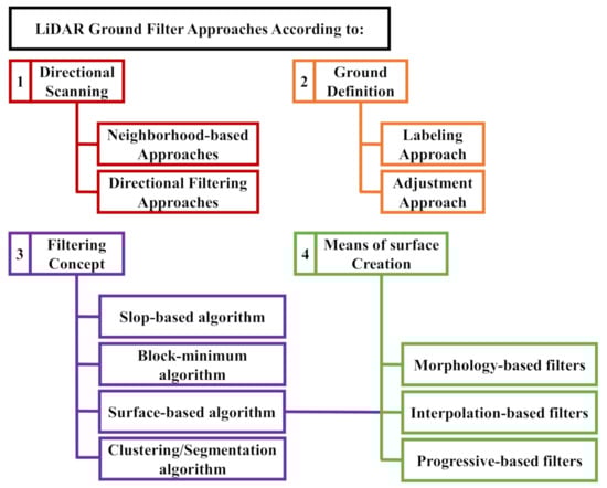
Figure 3.
LiDAR (Light Detection and Ranging) ground filtering different approaches.
Based on the filtering concept taxonomy, ground filters were grouped into slope-based, block-minimum, surface-based, and clustering/segmentation algorithms. The slope-based operator relied on comparing the slope of a LiDAR data point with its neighbors within a moving window. If the value exceeded a threshold range, the point was classified as a non-ground point [31]. Block-minimum filters detected the lowest point in height within a moving window and built a horizontal plane from this point. A height buffer from this plane was assumed so that local points were targeted as ground points if their height was within the identified buffer zone. Otherwise, the points were considered non-ground [51,52].
Surface-based algorithms were subdivided into morphology-based, interpolation-based, and progressive-based filters. Since these three types of filters apply different techniques to surfaces, they also fall under the fourth filtering category, with means of surface creation being the taxonomic criterion. A morphological filter detected the lowest elevation point within a window. Window points that fell within a band above this lowest point were grouped as ground points. Whereas interpolation-based approaches rely on producing an estimated terrain surface from LiDAR elevation points using an interpolation function and comparing the row points to the estimated surface for validation [31], progressive-based filters determine an initial subset of ground points as seed points, which are iteratively densified by merging neighbor points based on their mathematical relationship with original seed points in terms of elevation and slope [53]. Finally, clustering/segmentation algorithms embedded segmentation after the selection of seed points and before the iterative densification to expand the set of ground seed points to as many as possible for the filter to fit steep and mixed landscapes [47].
This study used the progressive TIN (Triangulated Inverse Network) densification approach, which was first introduced by Axelsson [53] for bare-earth extraction. The algorithm divides LiDAR point clouds into tiles and detects the lowest elevated point in each tile. These points are considered seed points, which contribute to creating a TIN as an initial terrain reference system. Potential points included within a triangle are added to seed points if the potential point’s distance to the TIN facet, in addition to the angle between the line connecting it to the nearest TIN’s vertex and the TIN facet itself, do not exceed predefined thresholds. This process is iterated until none of the remaining points meets these criteria. The remaining points after the final iteration are grouped as non-ground points.
2.3. Training Data Collection
In supervised classification, training data are labeled with classes of interest. The classifier’s effectiveness is intimately related to how well the training samples carry the class information [54]. Hence, training data should be representative and sufficient in quantity [19]. When considering the quantity of training samples, the spatial resolution of the data and the complexity of the landscape should be taken into account. This is especially the case when dealing with heterogeneous datasets acquired at fine spatial resolutions such as airborne LiDAR point clouds to ensure satisfactory classification results [20,55]. The training samples are usually collected from fieldwork or fine spatial resolution aerial photographs and satellite images [19]. However, analysts have abandoned in-situ training data collection, since it has been proven to be time consuming and laborious. Moreover, it does not always guarantee superior classification results. Thus, it is rather common and reasonable to derive training samples directly from the remotely sensed data using a priori knowledge of the scene [55,56].
In our case, either of the three sampling objects could be applied: single point, polygons of points, or seeding block training. In the single-point strategy, the training data for each class were collected as individual points, whereas in the second approach, they were selected by visually identifying and digitizing polygons of points, which may vary in size. The third approach relied on locating contiguous points with similar characteristics to the original seed point to ensure homogeneity of the collected training datasets [57]. The effect of the three strategies was more pronounced at fine spatial resolutions, and this impact was highlighted among classification accuracies of individual classes more than the overall accuracy. Small polygons of points were found to perform better in the case dealing with spatially heterogeneous classes, as they can easily capture information, therefore saving analysts’ time and effort [55]. In this paper, we applied an on-screen collection of training points using polygon objects.
2.4. Supervised Machine Learning Point-Based Classification
2.4.1. Maximum Likelihood (ML) Classifier
ML estimation is a probabilistic framework for solving the problem of density estimation by finding the probability density distribution function and its parameters that best describe the joint probability distribution of a set of observed data. It does so by defining multiple alternatives of distribution functions and their corresponding parameters and by maximizing the conditional probability (likelihood) of observing the data from the joint distribution at a certain density function and its parameters. This is a problem of fitting a machine learning model, where the selection of a distribution and its parameters that best describe a set of data represents the modeling hypothesis [58].
ML classifier is a parametric classifier since it uses a predefined probability distribution function (Gaussian) to describe data for each class. The parameters’ values (mean vector and covariance matrix) of each class’s underlying probability distribution are learned from the data using ML estimation [58]. Once trained, a ML classifier calculates the probability of a data point belonging to each class and subsequently assigns it the class with the highest probability. The simplicity of class assignment makes ML classification intuitively appealing [58,59]. ML was used in this study as a reference for classifier comparison, as it guarantees an optimal performance given the validity of the mutinormality assumption [59,60]. It also takes into account the mean vector and variance-covariance matrices within the class distribution of the training samples to define the multivariate normal probability model parameters, which are mathematically tractable and statistically desirable in a normal probability distribution [61,62]. ML often does not require large-sized training data even though the quality of estimation improves with the increased size of training samples [58]. Furthermore, ML simplifies the learning process into a linear machine learning algorithm due to being parametric [63].
2.4.2. Support Vector Machine (SVM) Classifier
SVM is a nonparametric classifier that approximates the probability distribution of the training samples without applying a predefined function. In most cases, kernel density estimation is used to approximate the probability density function of a continuous random variable. In kernel density estimation, a basis function (kernel) is used to interpolate a random variable’s probabilities and to control the sample records’ contribution in the probability estimation of each of them by weighting each based on its distance to a given query sample. On the other hand, the bandwidth controls the window of data records that participate in the probability estimation of each sample [58].
Brownlee [63] fully described the SVM algorithm as originally a maximal-margin classifier that looks for the most separable hyperplane to split point data into a set of desired classes based on their feature space. In the case of a 2D space, the hyperplane is visualized as a line for which the perpendicular distance to the closest data points represents a margin. These points are known as support vectors since they define the hyperplane and form the classifier accordingly. The larger the margin, the more discriminative the classifier becomes. Because remote sensing data are hard for perfect separation by nature, a soft-margin SVM is applied in this study to provide a certain degree of flexibility to the margin maximization constraint. The flexibility allows for some samples of the training data to break the separating line. In this way, a tuning parameter is introduced to determine the amount of tolerance allowed for the margin to violate the hyperplane. In other words, the tuning parameter represents the number of support vectors that are permitted to exist within the margin. A small parameter value indicates a lower violation of the hyperplane, a more sensitive algorithm to the training data, and a lower bias model.
SVM classifier implements kernels as transformation functions of the input space into higher dimensions for better class separation, which is recommended when dealing with a large feature space and/or heterogeneous landscapes. These kernels can be linear, polynomial, or radial. The last two are preferred for more accurate models, as they allow for maneuverability in separating curved or more complex classes. However, the polynomial degree and the gamma parameter that ranges from zero to one in the polynomial and radial kernels, respectively, should be maintained as minimally as possible to avoid overfitting problems.
2.4.3. Multilayer Perceptron (MLP) Artificial Neural Network Classifier
Brownlee [64] gave a broad picture of the nonparametric classifier as the most useful type of neural network in predictive machine learning modeling. A MLP neural network relies on artificial neurons as the network building block, where each neuron is a computational unit that uses an activation function to weight its inputs and bias. The whole structure of the neuron including its weighted inputs, bias, and outputs represents a perceptron. Optimization algorithms initially assign random weights to the neuron’s inputs, for which the summation determines the neuron’s output signal strength. Activation functions are responsible for the mathematical mapping between the input feeding a neuron and its output going to the next layer. An activation function can be a binary step, linear, or nonlinear; however, the latter is preferable to learn complex data sets [65].
A row of neurons represents a layer, and a network that consists of more than one layer is by definition a multilayer network, which has input (visible), hidden, and output layers. Each layer is defined by a number of neurons (nodes) and their activation functions. The input layer is the exposed portion of the network since it directly imports training data as numerical inputs. The feature space is a mandatory part of its definition. The hidden layers receive their input from the output signals of the visible layer. A network has at least a single hidden layer acting as its output layer, and it has several hidden layers in deep learning applications. The output layer is the last hidden layer in a network, where it produces the final prediction values of the problem being investigated. In a multiclass classification application, the number of neurons in the output layer must equal the number of land-use classes noticed in the scene [64]. Figure 4 shows a schematic of the structure of a MLP network.
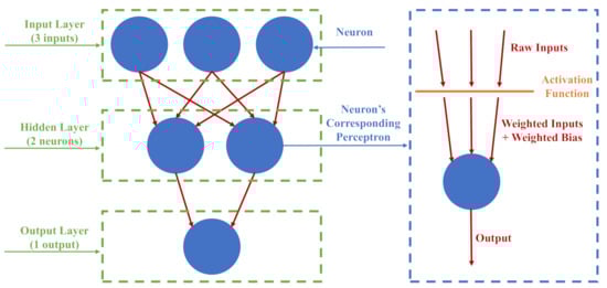
Figure 4.
Schematic structure of a simple MLP (Multilayer Perceptron Neural Network).
Prior to modeling, training data have to be numerical and scaled. Integer encoding and one-hot encoding were applied to represent ordinal and nominal data in a numerical format, respectively [66]. Data scaling could be achieved by either normalizing training samples to range from zero to one or by standardizing each feature so that it follows a standard normal distribution that has a mean of zero and a standard deviation of one [64].
The stochastic gradient descent optimization algorithm was used to train the model. It exposed each record in the training data to the network one at a time and applied forward processing by upward activation of the neurons until the final output. The model predicted the class of a training sample, compared it to the expected value, and calculated the error, which was backpropagated one layer at a time through the network to accordingly update the weights based on their contribution to the error. Loss and optimization functions were used to evaluate the model weights and alter their values, respectively. The backpropagation algorithm was repeated iteratively until it reached a set of weights that minimized the amount of prediction error [64,67]. A single round of network update in which the whole training instances participated is called an epoch, and in batch learning, a batch size demonstrated the number of observations to work through before updating the internal model weights. For example, a MLP model trained with 2000 samples for 1000 epochs and a batch size of 50 indicates that an individual epoch includes 40 model updates (2000/50), each occurring at every 50 records, and this process iterates for 1000 times [68]. A forward pass was eventually applied to the network after training to make predictions on unseen datasets to assess the model skill [64].
2.4.4. Bootstrap Aggregation (Bagging) Classifier
Combining predictions from multiple machine learning models into ensemble predictions improves their accuracies. Voting, Boosting, and Bagging are the most well-known combination methods. Voting algorithms apply several standalone submodels for classification (i.e., ML and SVM), whereas Boosting ensemble methods (i.e., AdaBoost) construct a series of submodels, each of which contributes corrections to its subsequent one. Meanwhile, Bagging divides training data into many groups of subsamples, with each subsample training the model separately. In a multiclass classification task, Voting, Boosting, or Bagging classifiers make predictions on unseen data by picking the most frequent class produced by the submodels. Stacked aggregation even enables weighting the submodels’ predictions based on their demonstrated accuracy and combines the results to build a single final output class [69].
Training subsamples generated in Bagging are called bootstraps and are created randomly with replacement. Therefore, a data element may be present more than once in the same bootstrap. This is beneficial when dealing with training data of limited size or sensitive classifiers with a high-variance performance for which the results are altered with the change in training samples (i.e., decision trees). In this way, Bagging ensures robust predictions and mitigates overfitting problems. The size of each bootstrap can be fixed to a certain number of observations. It can also be a fraction of the size of the original training dataset. However, the default for a subsample is to have the same size as the original training data. Each bootstrap trained a separate model, and the most frequent output class was eventually assigned to the point [67]. We also applied the Voting algorithm for more robust predictions, where the three classifiers (ML, SVM, and MLP) were the standalone submodels.
2.5. Model Validation
Predictions from datasets used to train machine learning models cannot be employed for evaluation to avoid overfitting problems. They may be biased, yielding pseud-optimistic results, and such a performance is never desired when testing the models with unseen data. The optimal method of assessment is to estimate the models’ performance on new data for which the classes are known in advance using statistical techniques [69]. Figure 5 summarizes the methods commonly used to evaluate the classification accuracy of machine learning algorithms. They all help to further adjust the models in case they show poor performance by altering data transformations, models, and configurations [67].
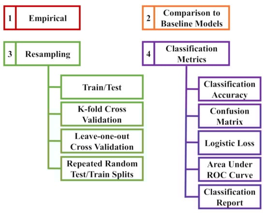
Figure 5.
Methods of assessment of machine learning classification algorithms (ROC: Receiver Operating Characteristic).
Empirical evaluation implies copying the configuration of models used in similar prediction problems, trained with more or less the same data size and already proved to produce satisfying results. It is commonly applied to construct and assess deep learning networks [64]. Baseline models are naive algorithms that serve as a point of comparison with more advanced machine learning models so that there is a means to determine whether these advanced models are genuinely superior. For example, baseline models are used as reference models in non-traditional classification problems, where the Random Prediction and Zero Rule algorithms are the most popular models to establish baseline performance [67].
Data splitting accommodates complex models that are slow to train [64]. Dividing the data into training and testing portions is the simplest form of data splitting; however, it does not take into consideration the variance expected when altering training and validation datasets presents tangible differences in the estimated model accuracy [69]. That is why k-fold cross-validation is the gold standard evaluation for machine learning approaches. It gained this reputation by splitting the data into a k number of folds, by holding out one subset for validation, and by using the rest to train the model. The algorithm terminates when all folds take turns as the held-out testing set. It produces a k number of different models where the entire data contributed to the fitting and evaluation processes, averaged the scores, and calculated their standard deviation assuming that they follow a Gaussian distribution. In this way, k-fold validation provides robust accuracy estimation on unseen data, with less bias than an individual train-test set. However, it is computationally expensive, and the choice of k may be tricky to secure a validation set and repetitions adequate for a reasonable evaluation. Hence, it is preferred in modest-sized prediction problems with sufficient computational hardware resources [64,69]. The leave-one-out approach is a special case of the k-fold cross-validation, where k is set to the number of records in the dataset, meaning that each fold contains a single sample. Although it creates the best possible learned models, it obviously takes longer processing time than the k-fold algorithm. Thus, it is the choice in small datasets or when the model’s skill estimation is critical [69]. The repeated random test splits method is similar to the k-fold approach since it randomly replicates the data division and assessment multiple times. It combines the benefits of the decline in running time and variance in the estimated model performance from the train-test splitting and k-fold cross-validation algorithms. It strikes a good balance when processing large and slow-trained datasets with a reduced bias at the same time [69].
On the other hand, evaluation metrics impact how the model performance is interpreted and compared [69]. Classification accuracy is the ratio of correct predictions to the whole ones made by the model. In spite of its simplicity, it is an unrepresentative measure for multiclass predictions since neither samples-per-class are usually constant nor all errors are equally important [67,69]. Therefore, it is usually accompanied by a confusion matrix. The latter is a square matrix where rows and columns represent predicted and actual classes, respectively, and each cell stores the number of predictions for each class. Ideally, it should be a diagonal matrix, as diagonal values (from top left to bottom right) are the correctly predicted samples whilst off-diagonal values represent the misclassified records. Consequently, it clearly reveals predictions and prediction errors for each class [67]. The logistic loss assigns scores to the predictions in proportional to their membership probability to a certain class. The area under the ROC (Receiver Operating Characteristics) curve measures the distinguishability of a model in a binary classification problem. A model has discrimination capabilities if the measure ranges from 0.5 to 1, indicating random and perfect predictions, respectively. Some modeling software and programming functions automatically generate classification reports that even include extra measures such as precision and recall [69]. We applied the train-test data splitting and k-fold cross-validation methods with the classification accuracy and confusion matrix metrics to evaluate the performance of the model developed in this study. They are the most suitable approaches concerning data size and the nature of the prediction problem addressed.
3. Experimental Work
All computations were processed by Python programming language v 3.7.4, on Spyder IDE (Integrated Development Environment) v 3.3.6, embedded in Anaconda Enterprise v 3.0. ERDAS IMAGINE v 2018 was used to visualize the 3D LiDAR point clouds. Additionally, LAStools were applied for LiDAR data conversion and metadata extraction. Data analysis was carried out on a workstation with the following specifications: Windows 10 Pro for workstations OS 64-bit, 3.2 GHz processor (16 CPUs), and memory of 131072MB RAM.
3.1. Study Area and Datasets
The LiDAR data covered a residential urban area of 33,000 m located in Rouge, a community neighborhood within the former suburb of Scarborough, east of Toronto city (Figure 6) (Screenshots were obtained from Google Maps in November 2020, and the neighborhoods shapefile was downloaded from the University of Toronto Libraries, Map and Data Library, Toronto Neighbourhoods (available from: https://mdl.library.utoronto.ca/collections/geospatial-data/toronto-neighbourhoods (accessed on 12 November 2020))). The point cloud (Figure 7) contained 1,976,164 points that were acquired at a 0.13 m spacing in 2015 by the multispectral Titan sensor, with three laser wavelengths: 532, 1064, and 1550 nm. The data were generated by the OptechLMS software that projected the 3D coordinates to the NAD (North American Datum) 1983 UTM (Universal Transverse Mercator) zone 17N coordinate system. We selected this study region because it contains different urban elements (i.e., asphalt, buildings, grass, and sidewalks) that commonly exist in residential urban morphologies and have been targeted for classification in similar studies for fair result comparison. We decided to limit the zone’s area to accommodate excessive processing time observed previously in the geo-registration process. Nevertheless, we managed this reduction in a way that still kept the region varied.
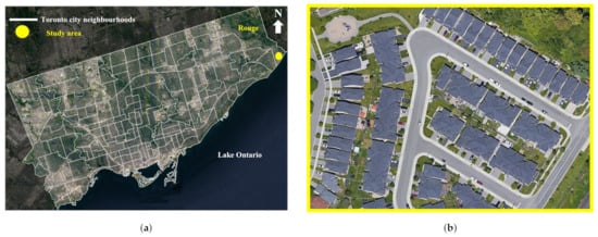
Figure 6.
Study region. (a) Location of the study zone in Toronto. (b) Study area zoomed-in.
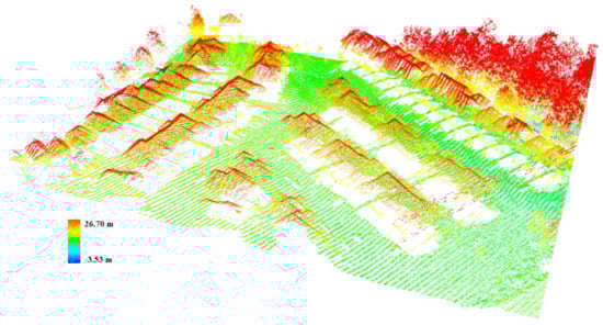
Figure 7.
LiDAR (Light Detection and Ranging) data by height values.
3.2. Data Geo-Registration
Despite the apparent satisfactory qualitative and quantitative validation of the geo-registration results conducted in [45], initial classification trials showed misalignment of the LiDAR point clouds. The misalignment stemmed from the incorrect inheritance of radiometric properties from the aerial photo to the point clouds. To solve this problem, we switched to the affine registration model at a spatial resolution of 40 cm instead of the third-order polynomial at a 200 cm spatial-resolution. For more robust results, we fused the CED (Canny Edge Detector) algorithm with the geo-registration workflow for scene abstraction instead of image clustering by running it on the PC filter output, as suggested by Megahed et al. [46]. We used the scikit-image library [70] to read images and detect edges, OpenCV [71] to save, and GDAL to georeference edges [72]. We converted the edges’ binary maps to zeros and ones instead of falses and trues, respectively, followed by another conversion to 8-bit images before exporting the results. We set the Gaussian blur (sigma parameter) to 2 and 0 for the LiDAR and aerial images, respectively. Whilst the double threshold values were adjusted to 0.1 and 0.3 for the LiDAR image, for the aerial photos, the values were 0 and 0.1.
3.3. Ground Filtering
The lasground-new tool [73] was used for bare-earth extraction out of the LiDAR point clouds. It is under the collection of LAStools software package. It is a revamped version of the original lasground tool that applies the progressive TIN densification approach. The lasground-new handles complicated terrain better than the lasground by increasing the default step size, which allows for removing most buildings in common cities. We applied the default step size for towns or flats, which is 25 m, to match the terrain of the residential study zone. It divided the data into 857,738 and 1,118,426 ground and non-ground points, respectively (Figure 8).
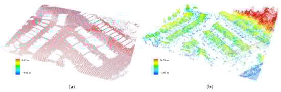
Figure 8.
Ground filtering of LiDAR data. (a) Ground points. (b) Non-ground points.
It is worth mentioning that outliers were removed from the raw LiDAR point clouds using the lasnoise tool [74] in a preprocessing step before the data geo-registration. The tool identifies a point as an outlier if its surrounding number of points within a 3D window is less than a predefined value. The window size and the minimum surroundings threshold values were kept as the tool’s default settings.
3.4. Training Samples Acquisition
Eight classes were observed in the study region: four ground classes—ark asphalt, light asphalt, sidewalks, and grass—and another four non-ground classes—buildings, vehicles, high vegetation, and low vegetation. Representative and well-distributed training data of 533,362 points were collected manually by digitizing polygons of points for each class on ERDAS IMAGINE (Figure 9). The pie charts in Figure 10 show the numerical and percentage breakdown of the acquired training samples.
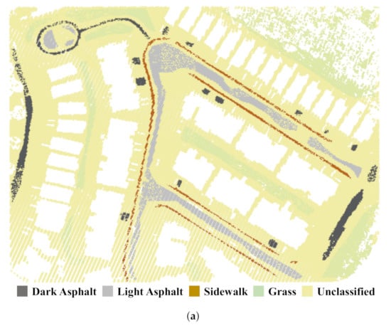
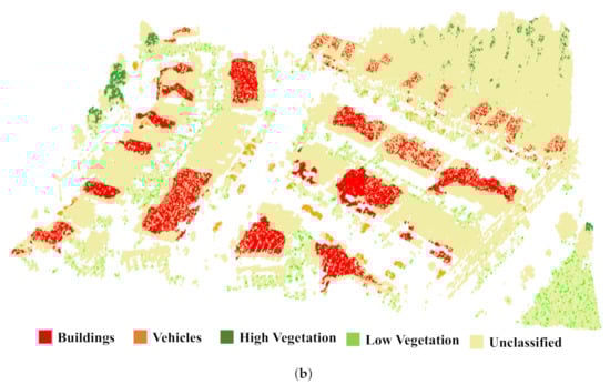
Figure 9.
Distribution of training data. (a) Ground samples. (b) Non-ground samples.
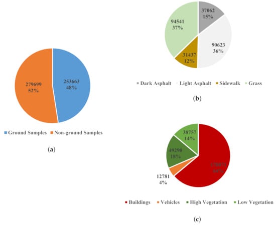
Figure 10.
Breakdown of training data. (a) Total samples. (b) Ground samples. (c) Non-ground samples.
3.5. Point-Based Classification
After data geo-registration and ground filtering, the LiDAR point clouds became attributed by the H (Height), I (Intensity), RGB (Red Green Blue), and NIR features. Additionally, NDVI was calculated as follows [75]:
The ML, SVM, and MLP neural networks classified the data considering four different scenarios for a thorough investigation of their effect on the classification accuracy:
- 1.
- H, I.
- 2.
- H, I, RGB.
- 3.
- H, I, RGB, NIR.
- 4.
- H, I, RGB, NIR, NDVI.
Once the best scenario was identified, the classification results were further improved by the Bagging ensemble technique using the abovementioned three classifiers and majority voting contributed to the production of the final map.
3.5.1. ML and SVM Classifications
Assuming a multivariate normal probability distribution in the ML classification, the likelihood was expressed as below [76]:
where
P(X|C): probability of a LiDAR point X belonging to class C,
n: number of features in class C,
V: variance-covariance matrix of n features in class C, and
M: vector of feature mean for n features in class C.
In contrast, in the SVM classification, the “scikit-learn” Python module [77] was used. The default SVM parameters were kept: the RBF kernel for its popularity and high mapping capabilities of input spaces, the trade-off parameter C of 1, and the scale option to calculate the kernel coefficient gamma as a scale measure using the feature dimension and values.
3.5.2. MLP Neural Network Classification
Keras Python library was used to create the MLP. It runs on top of the numerical platform TensorFlow to provide an interface to numerical libraries at the backend instead of direct execution of mathematical operations required for deep learning [64]. Neural networks cannot perform directly on categorical data; hence, the classes had to be converted to numerical values via the to_categorical function [78]. It involves label encoding, where each class is assigned an integer value, followed by a one-hot encoding, where a binary representation is added to avoid the assumption of having an ordinal relationship between classes [79].
A classical feedforward MLP was created by identifying a sequential model and by adding three fully connected layers using the Dense class. The input layer has 16 neurons, and the input dimension was set to the feature space, which is two, five, six, and seven, respectively, for each of the four scenarios. The hidden layer has 12 neurons, and both layers were activated by the ReLU (Rectified Linear Unit) function. It is linear for inputs larger than zero, which makes it easier to train and less likely to saturate. On the other hand, it is nonlinear for negative values that are output as zero [80,81]. Therefore, it provides a potential strategy to eliminate the vanishing gradients problem usually encountered while training deep feedforward networks, where the backpropagated error exponentially decreases at layers close to the input layer. Consequently, it results in a slow learning rate, premature convergence, and an imbalanced network by having more learning at layers close to the output layer [81]. The number of neurons in the output layer is equal to the number of output classes, which is four in the ground and non-ground LiDAR datasets. The layer was activated by the softmax nonlinear function, which is typically used in a multiclass classification problem, as it normalizes the outputs by converting the weighted sum values at each node into class membership probabilities that sum to one, following a multinomial probability distribution [82].
The model was compiled using the to_categorical logarithmic loss function [83] and Adam gradient descent optimization algorithm [84] and was fitted by the training samples’ features and classes over 100 batches and 100 epochs. As a rule of thumb, we started the training process with a few epochs (i.e., three epochs) and evaluated the predicted classes of the training data against their real ones. If the model yielded promising results, we optimized them by increasing the epochs; otherwise, we added more layers and/or neurons per layer. The final assessment was carried out on the validation dataset.
3.5.3. Bagging Classification
Eleven bootstraps were generated to carry out the Bagging classification. It secures a number of trained models adequate for robust classification results, and the odd number ensures a single most-frequent-class assignment to each point. The bootstraps were generated randomly with replacement, each with the same number of observations in the original training data. In other words, each of the 11 bootstraps randomly created for the dark asphalt class, for example, has 94,541 points (Figure 10). The same bootstraps were used for the three classifiers: ML, SVM, and MLP neural network for consistent comparison.
3.5.4. Accuracy Assessment
Since various machine learning classifiers were compared in this study, the same data splits were used for the models’ training and validation to ensure a consistent and fair comparison [67]. Two different validation and test sets were used to evaluate the models and did not contribute to the training process. The test data represent 1% of the data described in Figure 9 and provides an evaluation of the final model fit on the training samples [85]. The remaining 99% was further divided, as 80% was used to train the models, while 20% was used to denote the validation set used to assess a model fit on the training dataset while tuning model hyperparameters [85]. It is worth mentioning that all splits are stratified, meaning that the eight classes are represented proportionally to their original size in the data acquired manually on ERDAS IMAGINE. This guarantees a balanced representation of all classes, which is essential for good model learning as well as realistic and unbiased assessment results. Additionally, k-fold validation technique, with k set to 10, was applied to the MLP neural network model to accommodate its stochastic nature that is more highlighted than other machine learning algorithms due to its abovementioned mechanism of operation. Overall accuracy, per-class accuracy, and confusion matrices were the measures used for comparison.
To guarantee a reliable classifiers’ comparison, the three classifiers (ML, SVM, and MLP) used the same training, validation, and test data, on one hand. On the other hand, the Bagging approach ensures different training sets for each classifier to eliminate variance in the results.
4. Results
Early classification experiments revealed errors in the geo-registration performed in [45] using the third-order polynomial model. Figure 11 illustrates some of these errors featured by the displacement of sidewalks (Figure 11a) as well as misalignment of buildings and grasses (Figure 11c). The switch to the affine registration model at a spatial resolution of 40 cm along with the fusion of CED as described in [46] resulted in 3074 and 3045 candidate control points on the LiDAR and aerial images, respectively, which were matched into a set of 975 pairs of final control points. The whole processing took 14.7 h and yielded 1.78 and 1.19 pixels as model development and validation errors, respectively. Figure 11b,d display the effect of these modifications on correcting the displacement and misalignment of geo-registered points, respectively.
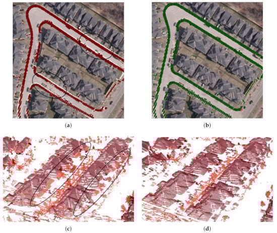
Figure 11.
Examples of geo-registration corrections: black ovals represent error locations. (a) Sidewalk displacement before corrections: aerial photo as basemap. (b) Sidewalk correct positioning: aerial photo as basemap. (c) Buildings/grass misalignment before corrections: NIR (Near Infrared), G (Green), and B (Blue) visualization. (d) Buildings/grass alignment after corrections: NIR, G, and B visualization.
Figure 12 outlines the overall classification accuracy on the validation and test sets for the four investigated scenarios. For the same classifier, each combination of features shows close accuracy values on both datasets: validation and test. Additionally, Figure 13 displays the results of the k-fold cross-validation performed on the MLP neural network classification models. The bars represent the mean accuracy of the ten folds calculated by averaging their results when each participated as the held-out testing set. The accuracy is shown separately for the ground and non-ground classifications since the models operated independently on both data after the ground filtering. The figures above the bars are the standard deviation of the ten accuracies, assuming a normal distribution. They are minimal, as the highest is ±0.26% for the non-ground classification of the second scenario except for the ±7.47% recorded by the ground classification of the first scenario.
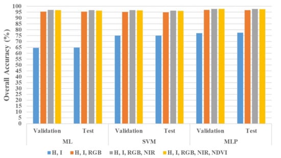
Figure 12.
Classification results on validation and test sets (ML: Maximum Likelihood, SVM: Support Vector Machine, H: Height, I: Intensity, RGB: Red Green Blue, NDVI: Normalized Difference Vegetation Index).
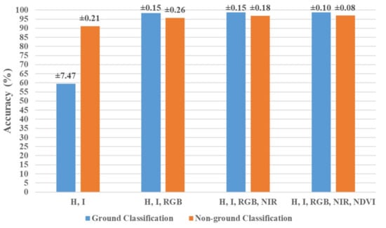
Figure 13.
K-fold cross-validation results of MLP neural network classification.
The skills achieved by the classifiers in each feature space group are illustrated in Figure 14. The overall accuracy (Figure 14a) of the first scenario that involved the I and H did not exceed 78%, which tangibly increased to cross 95% with the inclusion of the R, G, and B spectral properties in the feature space denoted by the second scenario. The overall accuracy increment looks uniform for the last three scenarios; however, the third feature combination that cumulatively appends the NIR provides the best scenario, with the largest overall accuracy surpassing 96%. The addition of the NDVI in the fourth feature set insignificantly lowered the overall accuracy, which was still above 96%.
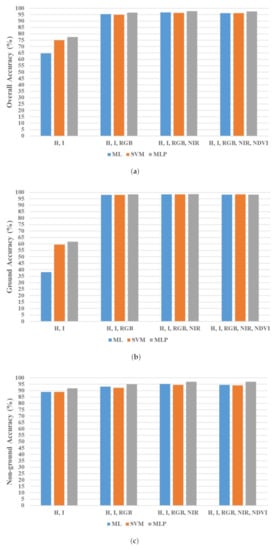
Figure 14.
Classification accuracy (test set). (a) Overall classification. (b) Ground accuracy. (c) Non-ground accuracy.
The influence of adding the radiometric characteristics to the feature space is better addressed in the ground classification (Figure 14b) than the non-ground (Figure 14c). The latter shows a relatively confined range of accuracies in all feature combinations, contrary to the ground classification, where the inclusion of the R, G, and B in the second scenario considerably improved the accuracy to around 98% after barely passing 60% in the first scenario. In addition, the ground classification shows accuracies higher than the non-ground in all feature combinations except the first one.
The MLP shows superiority over the ML and SVM classifiers, as it scores the highest overall accuracy of 97.75% with the third scenario’s feature space. This supremacy is proven in all scenarios and even highlighted in the ground classification, for which the accuracy passes 98% in the third scenario. The ML and SVM results are very similar; nevertheless, the ML displays preponderance in all scenarios except the first one. It achieves a 96.74% overall-accuracy versus 96.36% for the SVM in the third scenario. In terms of running time, Figure 15 illustrates the processing time required for the models’ training, validating, and testing in the four considered scenarios. The ML classifiers are the fastest predictive models in terms of the time expected for them to classify the data proportions directly with the feature space dimension. It gradually increases from 19 to 21, 24, and 25 min for the four feature combinations, respectively. The MLP networks show slightly longer processing times, as they run in 26–27 min. The SVM is the most computationally expensive classifier that noticeably slowly processes the data in 108 min for the first scenario. This time plunges to remain relatively steady for the rest of the scenarios, which take 43, 32, and 39 min, respectively.
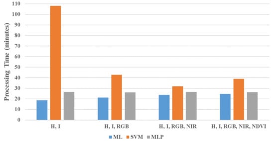
Figure 15.
Processing time.
Figure 16 provides a profound look at the per-class accuracy of the best scenario classification performed by the three classifiers. An individual class accuracy is exposed by producer and user accuracies. The first reflects the goodness of the classification itself, while the latter reveals the classification accuracy compared to the ground truth classes. Except for the vehicles and low vegetation classes, the bar charts display similar figures that are above 93%. The accuracies of the building, high vegetation, and light asphalt classes exceed 97%, and the sidewalk and grass accuracies even reached 100%. However, the vehicles and low vegetation classes have the lowest accuracies. The producer accuracies of the vehicle class are 61, 63, and 70%, and 89, 80, and 96% for the low vegetation class, as recorded by the three classifiers ML, SVM, and MLP, respectively.
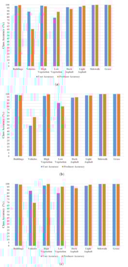
Figure 16.
Class accuracy (test set): scenario-3. (a) ML classification. (b) SVM classification. (c) MLP neural network classification.
Bagging classification results showed similar overall and per-class accuracy results. Therefore, we went directly to the Voting ensemble classification using the standalone predictions of ML, SVM, and MLP neural networks. Since the latter demonstrated the best accuracy results, LiDAR point clouds were assigned the MLP predictions in case of a draw frequency. The overall classification accuracy is 97.36%. This figure is higher than the maximum urban mapping accuracy to our knowledge so far, i.e., 95%, which was achieved by Morsy et al. [42] using costly multispectral LiDAR sensors. Moreover, it surpasses other accuracy figures that barely exceeded 90% using computationally expensive geometric feature spaces, as mentioned previously at the end of the Introduction section. Figure 17 displays the final map, for which a qualitative inspection reveals minor additional misclassification of high vegetation as buildings, light asphalt as dark asphalt, and buildings as high vegetation, marked as A, B, and C, respectively. The transmission towers were identified manually as non-ground scene features.
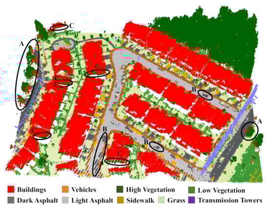
Figure 17.
Final LiDAR mapping: black ovals represent examples of misclassification (A: high vegetation as buildings, B: light asphalt as dark asphalt, C: buildings as high vegetation).
5. Discussion
As concluded in [45,46], it is better to apply the PC model for LiDAR and imagery data geo-registration on 2D images resampled at lower spatial resolutions to avoid computationally expensive data processing and high model development error values. However, including CED with the PC filter as a scene abstraction approach significantly reduces the model development error values (from 5.74 to 1.78 pixels using the affine model) when processing the data at high spatial resolutions (40 cm). It also applies to the model validation error figures but are not as noticeable (from 1.29 to 1.19 pixels). The double filtering eliminates noise that impacts precise edge detection. This multifilter fusion diminishes the gap between model development and validation errors. Consequently, it reconsiders registration models with data processed at high spatial resolutions that are excluded using the clustering scene abstraction approach due to their false indication of poor registration performance. Hence, the filter combination draws attention to decreasing the execution time when dealing with high spatial-resolution data (especially if they cover large study regions) by dividing them into tiles and/or by considering multithreading calculations.
On the other hand, the errors demonstrated in Figure 11 highlight the importance of a thorough qualitative post-registration inspection while validating the chosen empirical registration model. A model’s ability to minimize its development and validation errors should not be the sole criterion for model selection. For example, the third-order polynomial model produced the least and closest development and validation errors [45]; however, the model caused overparameterization that resulted in displacement and misalignment errors. Therefore, examining feature edges (i.e., building roofs and grasses) after ground filtering as well as a preliminary classification of some ground objects and matching them to a basemap are recommended practices for a reliable qualitative geo-registration assessment.
The results described in Figure 12 indicate the consistency of the classification models since the same scenario exhibits almost the same accuracy value when assessed separately by the validation and testing data. They prove the models’ consistency and precision and, consequently, the reliability of either set in demonstrating the classification accuracy. The k-fold cross-validation results shown in Figure 13 support this conclusion for the MLP neural networks, where the whole data not only contributed to the testing but also entirely participated in the training process yet produced compatible models with consistent results. However, a slim feature space, such as the first scenario, increases the variance of accuracies that is reflected by a high standard deviation to ±7.47% obtained in the ground classification. Nevertheless, since height values are non-distinctive for ground objects, they are a poor choice for being the sole feature in a feature space.
Generally, randomness is a characteristic in many machine learning algorithms due to stochastic domains that may include data with noise, random errors, or incomplete samples from a broader population (i.e., train/test data split). Furthermore, some algorithms use probabilistic decisions to ensure smooth learning that is generic enough to accommodate unseen data by fitting different models each time they run even on the same data [86]. Neural networks have additional sources of randomness as optimization classifiers that stochastically select subsequent areas of learning in the feature space based on areas that have been already searched. Moreover, the randomness in observation order and initial weights highly affects their internal decisions [87]. However, the results of the k-fold cross-validation (Figure 13) confirm robust MLP models thanks to adequate and representative training data.
Expanding the poor LiDAR feature space to include the R, G, and B radiometric signatures as in the second scenario boomed the overall mapping accuracy (Figure 1a). Since the naked-eye scene visualization (Figure 6b) is discriminative, this addition to the H and I features enabled the classifiers to differentiate between buildings, sidewalks, dark and light asphalts. Moreover, consideration of the NIR spectral property in the third scenario provided a better recognition of the green objects such as grasses, and high and low vegetation, which improved the overall accuracy. On the other hand, the intangible contribution of the NDVI is justified as it is a calculated index derived from the already included NIR and R features, and this repetition did not add significant value to the classification accuracy. As described previously in this section, the first scenario represents a 1D feature space in the ground classification. Therefore, its accuracy (Figure 14b) was influenced by adding R, G, and B to the feature space in the second scenario more than the non-ground classification, where the H values do represent a discriminative feature (Figure 14c). It also explains the plunge in accuracy of the ground classification compared to the non-ground in the same scenario.
The higher accuracy figures denoted by the ML over the SVM classifier, despite being very close, support the validity of assuming a Gaussian probability data distribution, which makes ML more advisable than SVM since the latter requires substantial time for training and hyperparameter fine-tuning. However, this conclusion does not apply to 1D feature spaces, as in the ground classification of the first scenario, where ML dipped the accuracy to 38.09% compared to 59.47% by SVM (Figure 14b) and subsequently lowered the overall accuracy to 64.76% compared to 74.97% of SVM (Figure 14a). On the other hand, the outperformance of the MLP networks reflects their flexibility in addressing nonlinear predictive problems due to their capacity of approximating unknown functions, which justifies their outstanding accuracy figures even with 1D feature spaces. Its overall accuracy reached 77.59% in the first scenario, which is a considerably better performance than ML and SVM, given the same situation.
Another distinguishing feature of the MLP neural networks is the updating of the parameters and the backpropagation of errors at each epoch, which eventually stabilizes the models by ensuring good learning without overfitting or underfitting. Figure 18 shows the learning curves of the MLP network classification of the best scenario, i.e., the third feature combination. The plots reveal an association between the model error evaluated on the training and validation sets and the number of epochs used in the model configuration. An underfit model shows a better performance (lower loss) on the training than the validation data, with a noticeably poor validation performance that either declines or levels off with the increase in epochs. The performance decline can be solved by increasing the number of epochs and/or the training data size, whereas expanding the model capacity to include more neurons and/or hidden layers may help to solve the leveling-off problem. On the other hand, an overfit network gives improved accuracies on the training and validation data, with the validation curve overlapping with the training’s and then deviating from it with the increase of epochs. Terminating the model at the inflection point and/or introducing more training data may solve the issue. Therefore, the plots in Figure 18 confirm a good fit since the models perform well on both sets, in which the curves stabilize around the same loss value while the epochs grow.
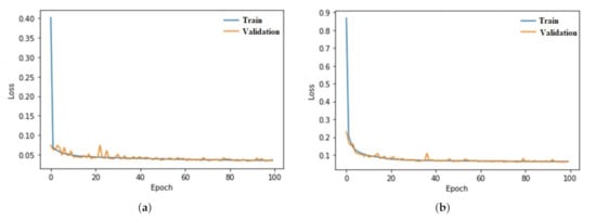
Figure 18.
MLP neural network learning curves: scenario 3. (a) Ground training. (b) Non-ground training.
ML is a systematic classifier that straightforwardly follows Equation (1), where the feature space dimension directly affects the size of the mean vector and variance-covariance matrix. Therefore, a progressively increasing processing time is observed along with the four feature combinations (Figure 15). Despite the highest model skills recorded by the MLP networks, they are slightly more time-consuming than ML, with a training period occupying the vast majority of the total processing time regardless of the feature space dimension. The run time almost did not change along with the given scenarios, as it is connected to the network structure that remained the same in all feature combinations. Nevertheless, the models once created carried out predictions quickly (i.e., 1.7 min in the classification using the best scenario). SVM spends a long time building hyperplanes to differentiate various classes, in general. Such a drawback is significantly highlighted when training the models using a narrow feature space as in the ground classification of the first scenario, the processing of which took twice the time needed for the non-ground data.
The per-class accuracies obtained by the three classifiers (Figure 16) indicate satisfying results, except for the vehicles for which the producer accuracy figures were notably lower due to the class misclassification with the low vegetation. This consequently decreased the non-ground classification accuracies (Figure 14c) as compared to the ground ones (Figure 14b). Vehicles are small-sized mobile urban features with no distinguishable spectral characteristics. They are unlikely to maintain their locations on scenes captured by different sensors at various times as in this geo-registration case, where the LiDAR point clouds were obtained in 2015 independently from the aerial photo that was captured a year ahead. Figure 19 shows how the vehicle points inherited the radiometric properties of the ground surfaces where they usually park (i.e., grassy sidewalks). As non-ground objects, vehicles were closer to the low vegetation class spectrally and geometrically, given that the height was the only geometric feature considered in the classification. Considering additional geometric properties in the classification feature space can help eliminate this misclassification. ML and MLP classifiers gave relatively close vehicle-class accuracies, notably higher than the SVM that hardly creates discriminative hyperplanes to differentiate between similar classes [29,88].
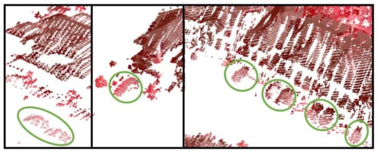
Figure 19.
Radiometric characteristics of vehicles: green ovals represent vehicle locations—NIR, G, and B visualization.
Bagging classification results were similar, indicating a good training dataset; however, Bagging took a substantial amount of processing (>4 h) to classify the LiDAR data 11 times. Hence, neither the Bagging classification nor the k-fold cross-validation (processing ten folds also exceeded four hours) are advisable when having adequate training data, which were already proven reliable on validation and testing data. The transmission towers in the final map (Figure 17) do not have sufficiently frequent appearance in the study area to be considered an independent class. Their points inherited vegetation radiometric properties after geo-registration, and their height misled the classifiers to predict them as high vegetation. Therefore, they were picked up manually and reclassified.
Figure 20 plots the locations of the extra misclassification examples denoted in Figure 17 on the corresponding aerial photo that contributed to the geo-registration. Misclassification of some high vegetation points as buildings (A examples) is due to aerial and LiDAR data acquired at different times. These high trees were not planted at the time of obtaining the aerial image, so they inherited the dark asphalt’s spectral characteristics. Eventually, they became similar to the buildings’ radiometric and geometric properties, as they also share similar height values. The B examples on the aerial photo mark spots of shadows that belong to light asphalt but are wrongly predicted as dark asphalt, as the latter radiometrically resemble shadows. Finally, the C examples address the misprediction of some edge-building points as high trees. It is a result of an inaccurate orthorectification of the aerial image, where the building facades are still observed. The zoom-in in Figure 20 exhibits an overlay of the geo-referenced LiDAR and aerial images, where the inexact orthorectification shifted the roofs from their correct projection and revealed the interfaces. Consequently, the building points located on the edges acquired the spectral characteristics of the facades and surrounding surfaces that are planted, leading to being wrongly assigned to high vegetation, especially with close height ranges.
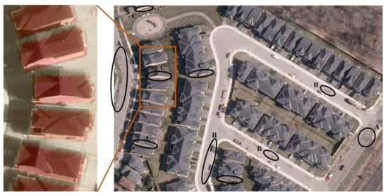
Figure 20.
Examples of misclassification by external factors (A: different acquisition time, B: shadow, C: inexact orthorectification) on corresponding aerial photo: the zoom-in shows a height LiDAR-image overlay in transparent orange layer.
The shadow effect appears in the per-class accuracy results (Figure 16), where the dark asphalt figures are slightly below the rest of the classes. On the other hand, the impact of the high-vegetation/buildings misclassification due to different acquisition times and inaccurate orthorectification of aerial data does not show up in the accuracy results. That is because LiDAR point clouds at such locations were not included in the training data (Figure 9b), of which the validation and testing sets are a part (Figure 10). The abovementioned impacts are the drawbacks associated with the geo-registration of airborne LiDAR data to aerial/satellite images. Nevertheless, it provides an affordable yet accurate means of densifying classification feature spaces for better mapping.
In the end, we can summarize the contribution of our proposed study to the fusion of airborne LiDAR and imagery data in the classification of urban land-uses as follows:
- Referring to the geo-registration of both data types by the PC model and scene abstraction algorithm that locate control points, which are not limited to points on traditional linear elements and intersections. The approach does not require data to be georeferenced, applies empirical registration models without knowing the physical model characteristics, and overcomes the problem of airborne LiDAR data not coming with onboard optical images collected during the same flight mission. Full details about the geo-registration approach are found in [46].
- Suggesting the inclusion of the CED to the PC filter for a more concise detection of geo-registration primitives. This study highlights the importance of a thorough qualitative inspection of the abovementioned geo-registration method’s results, as empirical models might cause overparameterization that cannot be quantitatively revealed.
- Introducing a new data fusion approach to LiDAR point cloud classification that constructs radiometric-based feature spaces from spectral characteristics inherited from aerial images. With affordable sensors and computationally inexpensive feature spaces that include only I and H from LiDAR data and RGB, NIR, and NDVI from aerial photos, we achieved a mapping accuracy over 95% with a conventional classifier as ML and over 97% with MLP.
- Investigating different combinations of the features as mentioned above with various commonly known classifiers: ML, SVM, and MLP in regards to the logic behind each classifier, overall and per-class accuracies, and processing time. This comparison helped exclude SVM and derived features (i.e., NDVI) from enhancing the mapping accuracies.
For future work, we recommend applying shadow-removal and post-orthorectification strategies to aerial data before geo-registration to eliminate the impact of LiDAR point clouds receiving incorrect radiometric properties and thus to minimize misclassification errors. In addition, we suggest investigating the expansion of feature spaces by performing an object-based classification to allow geometric features and/or extra radiometric ones from hyperspectral imagery data.
6. Conclusions
This study examines the effect of including different radiometric properties along with the height values on the classification results of LiDAR point clouds of an urban morphology. The morphology comprises classical urban-residential objects: sidewalks, grasses, dark and light asphalt, buildings, vehicles, and high and low vegetations. In contrast to traditional point-based classification work that relies on high-dimensional geometric-oriented feature space, our research uses spectral properties inherited from an aerial photo after geo-registering it to the LiDAR point clouds to form different feature combinations. That provides an affordable approach towards rich feature spaces instead of the computationally expensive conventional ones and the costly multispectral airborne LiDAR sensors. The geo-registration added R, G, B, and NIR to the LiDAR’s I and H feature space as well as the calculated NDVI.
We considered four scenarios for ground and non-ground classifications. The first scenario started with H and I and then incrementally involved RGB, NIR, and NIR for the remaining feature combinations. We applied three supervised machine learning algorithms to classify the scene, i.e., ML, SVM, and MLP neural networks, and used three separate sets out of the original LiDAR data for model training, validation, and testing. The validation and testing results of the three classifiers and the k-fold cross-validation of the MLP networks showed consistent accuracies, which indicated that the models were reliable for the prediction of unseen data.
The best classifying features were those of the third scenario. The NDVI is already derived from the NIR and R signatures, so it did not add to the results. The best scenario gave overall accuracies of 96.74, 96.36, and 97.75% for the three classifiers. The MLP results were the most outperforming, followed by the ML algorithm. That is because of the layering feature of MLP that approximates nonlinear prediction problems and the ML’s valid assumption about the normal distribution of data. The SVM was not as promising as ML and MLP, especially with mixed classes and narrow feature spaces, where it struggled to build discriminative hyperplanes. The three classifiers processed the data in 24, 32, and 26 min, respectively. The run time of the ML, SVM, and MLP models relied on the feature dimension, feature dimension and complexity of classes, and the network structure, respectively.
The per-class accuracies showed a low-vegetation/vehicle and dark/light-asphalt misclassifications. The first is due to vehicles acquiring the properties of grassy parking surfaces, and the latter is a consequence of the shadow existence in the aerial image. Moreover, the LIDAR/imagery data acquisition at different times and the inaccurate orthorectification of the aerial photo resulted in misclassification of the buildings and high-vegetation classes. These mispredictions highlight the shortcomings of the LiDAR/aerial data geo-registration as well as the importance of a thorough qualitative post-classification assessment. The inclusion of geometric indices can eliminate the abovementioned misclassifications. Nevertheless, the addition of traditional spectral signatures such as R, G, B, and NIR to the LiDAR’s height values boomed the mapping results to exceed 97%. Finally, the Bagging classification and k-fold cross-validation exceeded four hours to process the data. Hence, they are not recommended practices in cases with sufficient training samples. The majority voting results of the three classifiers produced an overall accuracy of 97.36%.
Author Contributions
A.S. and W.Y.Y. conceived the study and commented on the article; Y.M. wrote the code, performed the analysis, and wrote the article. All authors have read and agreed to the published version of the manuscript.
Funding
This research was funded by the Discovery Grant from the Natural Sciences and Engineering Research Council of Canada (NSERC) (RGPIN-2015-03960), the FCE Start-up Fund of the Hong Kong Polytechnic University (BE2U), and the Early Career Scheme (Project Number: 25213320) by the Research Grants Council of the Hong Kong Special Administrative Region.
Acknowledgments
The authors would like to thank Ernest Ho for his thorough proofreading and valuable suggestions.
Conflicts of Interest
The authors declare no conflict of interest.
Abbreviations
The following abbreviations are used in this manuscript:
| AI | Artificial Intelligence |
| CED | Canny Edge Detector |
| CRF | Conditional Random Field |
| DIM | Dense Image Matching |
| GBT | Gradient Boosted Trees |
| GNB | Gaussian Naive Bayes |
| H | Height |
| HMP | Hierarchical Morophological Profile |
| HSV | Hue Saturation Value |
| I | Intensity |
| IDE | Integrated Development Environment |
| IDW | Inverse Distance Weighted |
| IMMW | Iterative Majority Moving Window |
| KNN | K-Nearest Neighbors |
| LiDAR | Light Detection and Ranging |
| LULC | Land Use Land Cover |
| MIR | Mid Infrared |
| ML | Maximum Likelihood |
| MLP | Multilayer Perceptron Neural Network |
| MP | Morophological Profile |
| NAD | North American Datum |
| NDSM | Normalized Digital Surface Model |
| NDVI | Normalized Difference Vegetation Index |
| NIR | Near Infrared |
| NN | Nearest Neighbor |
| PC | Phase Congruency |
| PCA | Principal Component Analysis |
| PCR | Principal Component Regression |
| ReLU | Rectified Linear Unit |
| RF | Random Forest |
| RGB | Red Green Blue |
| ROC | Receiver Operating Characteristics |
| SVM | Support Vector Machine |
| TIN | Triangulated Inverse Network |
| UAS | Unmanned Aircraft System |
| UAV | Unmanned Aerial Vehicle |
| UTM | Universal Transverse Mercator |
References
- World Health Organization. Hidden cities: Unmasking and overcoming health inequities in urban settings. In Centre for Health Development and World Health Organization; World Health Organization: Geneva, Switzerland, 2010. [Google Scholar]
- Güneralp, B.; Reba, M.; Hales, B.U.; Wentz, E.A.; Seto, K.C. Trends in urban land expansion, density, and land transitions from 1970 to 2010: A global synthesis. Environ. Res. Lett. 2020, 15, 044015. [Google Scholar] [CrossRef]
- Oliinyk, O.; Serhiienko, L.; Legan, I. Public administration of economic and ecological urbanization consequences. Fundam. Appl. Res. Pract. Lead. Sci. Sch. 2020, 37, 27–33. [Google Scholar]
- Long, T.; Jiao, W.; He, G.; Zhang, Z.; Cheng, B.; Wang, W. A generic framework for image rectification using multiple types of feature. ISPRS J. Photogramm. Remote. Sens. 2015, 102, 161–171. [Google Scholar] [CrossRef]
- Lefsky, M.A.; Cohen, W.B.; Parker, G.G.; Harding, D.J. Lidar remote sensing for ecosystem studies: Lidar, an emerging remote sensing technology that directly measures the three-dimensional distribution of plant canopies, can accurately estimate vegetation structural attributes and should be of particular interest to forest, landscape, and global ecologists. BioScience 2002, 52, 19–30. [Google Scholar]
- Dalponte, M.; Bruzzone, L.; Gianelle, D. Fusion of hyperspectral and LIDAR remote sensing data for classification of complex forest areas. IEEE Trans. Geosci. Remote. Sens. 2008, 46, 1416–1427. [Google Scholar] [CrossRef]
- Jaboyedoff, M.; Oppikofer, T.; Abellán, A.; Derron, M.H.; Loye, A.; Metzger, R.; Pedrazzini, A. Use of LIDAR in landslide investigations: A review. Nat. Hazards 2012, 61, 5–28. [Google Scholar] [CrossRef]
- Radiohead-House of Cards. Light Detection and Ranging (LiDAR). [University Lecture]; Portland State University: Portland, OR, USA, 2017. [Google Scholar]
- NOAA. What Is LIDAR? National Ocean Service Website. Available online: http://oceanservice.noaa.gov/facts/lidar.html (accessed on 8 March 2020).
- Wu, H.; Li, Y.; Li, J.; Gong, J. A two-step displacement correction algorithm for registration of lidar point clouds and aerial images without orientation parameters. Photogramm. Eng. Remote. Sens. 2010, 76, 1135–1145. [Google Scholar] [CrossRef]
- Dalponte, M.; Bruzzone, L.; Gianelle, D. Tree species classification in the Southern Alps based on the fusion of very high geometrical resolution multispectral/hyperspectral images and LiDAR data. Remote. Sens. Environ. 2012, 76, 123–258. [Google Scholar] [CrossRef]
- Tonolli, S.; Dalponte, M.; Neteler, M.; Rodeghiero, M.; Vescovo, L.; Gianelle, D. Fusion of airborne LiDAR and satellite multispectral data for the estimation of timber volume in the Southern Alps. Remote. Sens. Environ. 2011, 115, 2486–2498. [Google Scholar] [CrossRef]
- Christiansen, M.P.; Laursen, M.S.; Jørgensen, R.N.; Skovsen, S.; Gislum, R. Designing and testing a UAV mapping system for agricultural field surveying. Sensors 2017, 17, 2703. [Google Scholar] [CrossRef] [PubMed]
- Qin, X.; Wu, G.; Lei, J.; Fan, F.; Ye, X.; Mei, Q. A novel method of autonomous inspection for transmission line based on cable inspection robot lidar data. Sensors 2018, 18, 596. [Google Scholar] [CrossRef] [PubMed]
- Kumar, G.A.; Patil, A.K.; Chai, Y.H. Alignment of 3D point cloud, CAD model, real-time camera view and partial point cloud for pipeline retrofitting application. In Proceedings of the 2018 International Conference on Electronics, Information, and Communication (ICEIC), Honolulu, HI, USA, 24–27 January 2018; pp. 1–4. [Google Scholar]
- Bonatti, R.; Wang, W.; Ho, C.; Ahuja, A.; Gschwindt, M.; Camci, E.; Kayacan, E.; Choudhury, S.; Scherer, S. Autonomous aerial cinematography in unstructured environments with learned artistic decision-making. J. Field Robot. 2018, 37, 606–641. [Google Scholar] [CrossRef]
- Völz, B.; Behrendt, K.; Mielenz, H.; Gilitschenski, I.; Siegwart, R.; Nieto, J. A data-driven approach for pedestrian intention estimation. In Proceedings of the 2016 IEEE 19th International Conference on Intelligent Transportation Systems (ITSC), Rio de Janeiro, Brazil, 1–4 November 2016; pp. 2607–2612. [Google Scholar]
- Bhatta, B. Analysis of Urban Growth and Sprawl from Remote Sensing Data; Springer Science & Business Media: Berlin/Heidelberg, Germany, 2010. [Google Scholar]
- Lu, D.; Weng, Q. A survey of image classification methods and techniques for improving classification performance. Int. J. Remote Sens. 2007, 28, 823–870. [Google Scholar] [CrossRef]
- Van Genderen, J.L. Advances in environmental remote sensing: Sensors, algorithms, and applications. Int. J. Digit. Earth 2011, 4, 446–447. [Google Scholar] [CrossRef]
- Expert System. What Is Machine Learning? A Definition. Expert System Website. Available online: https://expertsystem.com/machine-learning-definition (accessed on 6 May 2020).
- Schowengerdt, R.A. Remote Sensing, Models, and Methods for Image Processing, 3rd ed.; Academic Press: Cambridge, MA, USA, 2007. [Google Scholar]
- El-Ashmawy, N.T.H. Innovative Approach for Automatic Land Cover Information Extraction from LiDAR Data. Ph.D. Dissertation, Ryerson University, Toronto, ON, Canada, 2015. [Google Scholar]
- Cortijo, F.; de la Blanca, N.P. Image classification using non-parametric classifiers and contextual information. Int. Arch. Photogramm. Remote Sens. 1996, 31, 120–124. [Google Scholar]
- Brownlee, J. A Tour of Machine Learning Algorithms. Machine Learning Mastery Website. Available online: https://machinelearningmastery.com/a-tour-of-machine-learning-algorithms (accessed on 14 August 2020).
- Alba, G.E.R.M.A.N. Remote sensing classification algoritms analysis applied to land cover change. Mario Gulich Inst. Argent. 2014.
- Atkinson, P.M. Sub-pixel target mapping from soft-classified, remotely sensed imagery. Photogramm. Eng. Remote. Sens. 2005, 71, 839–846. [Google Scholar] [CrossRef]
- Myint, S.W.; Gober, P.; Brazel, A.; Grossman-Clarke, S.; Weng, Q. Per-pixel vs. object-based classification of urban land cover extraction using high spatial resolution imagery. Remote Sens. Environ. 2011, 115, 1145–1161. [Google Scholar] [CrossRef]
- Yan, W.Y.; Shaker, A.; El-Ashmawy, N. Urban land cover classification using airborne LiDAR data: A review. Remote Sens. Environ. 2015, 158, 295–310. [Google Scholar] [CrossRef]
- Bater, C.W.; Coops, N.C. Evaluating error associated with lidar-derived DEM interpolation. Comput. Geosci. 2009, 35, 289–300. [Google Scholar] [CrossRef]
- Liu, X. Airborne LiDAR for DEM generation: Some critical issues. Prog. Phys. Geogr. 2008, 32, 31–49. [Google Scholar]
- Guo, Q.; Li, W.; Yu, H.; Alvarez, O. Effects of topographic variability and lidar sampling density on several DEM interpolation methods. Photogramm. Eng. Remote Sens. 2010, 76, 701–712. [Google Scholar] [CrossRef]
- Jochem, A.; Höfle, B.; Rutzinger, M.; Pfeifer, N. Automatic roof plane detection and analysis in airborne lidar point clouds for solar potential assessment. Sensors 2009, 9, 5241–5262. [Google Scholar] [CrossRef]
- El-Ashmawy, N.; Shaker, A. Raster vs. point cloud LiDAR data classification. Int. Arch. Photogramm. Remote Sens. Spat. Inf. Sci. 2014, 40, 79. [Google Scholar] [CrossRef]
- Lodha, S.K.; Fitzpatrick, D.M.; Helmbold, D.P. Aerial lidar data classification using adaboost. In Proceedings of the Sixth International Conference on 3-D Digital Imaging and Modeling-IEEE, Montreal, QC, Canada, 21–23 August 2007; pp. 435–442. [Google Scholar]
- Gao, Y.; Li, M.C. Airborne lidar point cloud classification based on multilevel point cluster features. Int. Arch. Photogramm. Remote Sens. Spat. Inf. Sci. 2020, 42, 1231–1237. [Google Scholar] [CrossRef]
- Wang, C.; Shu, Q.; Wang, X.; Guo, B.; Liu, P.; Li, Q.C. A random forest classifier based on pixel comparison features for urban LiDAR data. ISPRS J. Photogramm. Remote Sens. 2019, 148, 75–86. [Google Scholar] [CrossRef]
- Zaboli, M.; Rastiveis, H.; Shams, A.; Hosseiny, B.; Sarasua, W.A. Classification of mobile terrestrial Lidar point cloud in urban area using local descriptors. Int. Arch. Photogramm. Remote Sens. Spat. Inf. Sci. 2019, 42, 1117–1122. [Google Scholar] [CrossRef]
- Niemeyer, J.; Rottensteiner, F.; Sörgel, U.; Heipke, C.A. Hierarchical higher order crf for the classification of airborne lidar point clouds in urban areas. Int. Arch. Photogramm. Remote Sens. Spat. Inf. Sci. 2016, 41, 655–662. [Google Scholar] [CrossRef]
- Huo, L.Z.; Silva, C.A.; Klauberg, C.; Mohan, M.; Zhao, L.J.; Tang, P.; Hudak, A.T. Supervised spatial classification of multispectral LiDAR data in urban areas. PLoS ONE 2018, 13, e0206185. [Google Scholar] [CrossRef]
- Morsy, S.; Shaker, A.; El-Rabbany, A. Multispectral LiDAR data for land cover classification of urban areas. Sensors 2017, 17, 958. [Google Scholar] [CrossRef]
- Morsy, S.; Shaker, A.; El-Rabbany, A. Clustering of multispectral airborne laser scanning data using Gaussian decomposition. Int. Arch. Photogramm. Remote Sens. Spat. Inf. Sci. 2017, 42, 269–276. [Google Scholar] [CrossRef]
- Becker, C.; Häni, N.; Rosinskaya, E.; d’Angelo, E.; Strecha, C. Classification of aerial photogrammetric 3D point clouds. arXiv 2017, arXiv:1705.08374. [Google Scholar] [CrossRef]
- Zhou, M.; Kang, Z.; Wang, Z.; Kong, M. Airborne lidar point cloud classification fusion with dim point cloud. Int. Arch. Photogramm. Remote Sens. Spat. Inf. Sci. 2020, 43, 375–382. [Google Scholar] [CrossRef]
- Megahed, Y.; Yan, W.Y.; Shaker, A. Semi-automatic approach for optical and LiDAR data integration using phase congruency model at multiple resolutions. Int. Arch. Photogramm. Remote Sens. Spat. Inf. Sci. 2020, 43, 611–618. [Google Scholar] [CrossRef]
- Megahed, Y.; Yan, W.Y.; Shaker, A. A phase-congruency-based scene abstraction approach for 2d-3d registration of aerial optical and LiDAR images. IEEE J. Sel. Top. Appl. Earth Obs. Remote Sens. 2020, 964–981. [Google Scholar] [CrossRef]
- Zhang, J.; Lin, X. Filtering airborne LiDAR data by embedding smoothness-constrained segmentation in progressive TIN densification. ISPRS J. Photogramm. Remote Sens. 2013, 81, 44–59. [Google Scholar] [CrossRef]
- Li, Y.; Yong, B.; Wu, H.; An, R.; Xu, H.; Xu, J.; He, Q. Filtering airborne lidar data by modified white top-hat transform with directional edge constraints. Photogramm. Eng. Remote Sens. 2014, 80, 133–141. [Google Scholar] [CrossRef]
- Meng, X. Determining Urban Land Uses through Building-Associated Element Attributes Derived from Lidar and Aerial Photographs. Ph.D. Dissertation, Texas State University, San Marcos, YX, USA, 2010. [Google Scholar]
- Shan, J.; Aparajithan, S. Urban DEM generation from raw LiDAR data. Photogramm. Eng. Remote. Sens. 2005, 71, 217–226. [Google Scholar] [CrossRef]
- Sohn, G.; Dowman, I.J. A model-based approach for reconstructing a terrain surface from airborne LIDAR data. Photogramm. Rec. 2008, 23, 170–193. [Google Scholar] [CrossRef]
- Milledge, D.G.; Lane, S.N.; Warburton, J. The potential of digital filtering of generic topographic data for geomorphological research. Earth Surf. Process. Landf. 2009, 34, 63–74. [Google Scholar] [CrossRef]
- Axelsson, P.E. DEM generation from laser scanner data using adaptive TIN models. Int. Arch. Photogramm. Remote. Sens. Spat. Inf. Sci. 2000, 32 Pt B4/1, 110–117. [Google Scholar]
- GIS Geography. Image Classification Techniques in Remote Sensing. GIS Geography Website. Available online: http://gisgeography.com/image-classification-techniques-remote-sensing (accessed on 5 March 2020).
- Chen, D.; Stow, D. The effect of training strategies on supervised classification at different spatial resolutions. Photogramm. Eng. Remote Sens. 2002, 68, 1155–1162. [Google Scholar]
- Huang, X.; Weng, C.; Lu, Q.; Feng, T.; Zhang, L. Automatic labelling and selection of training samples for high-resolution remote sensing image classification over urban areas. Remote Sens. 2015, 7, 16024–16044. [Google Scholar] [CrossRef]
- Jensen, J.R. Introductory Digital Image Processing: A Remote Sensing Perspective, 2nd ed.; Prentice-Hall Inc.: Upper Saddle River, NJ, USA, 1996. [Google Scholar]
- Brownlee, J. Probability for machine learning: Discover how to harness uncertainty with Python. In Machine Learning Mastery; 2000; Available online: https://books.google.com.hk/books?id=uU2xDwAAQBAJ&pg=PP1&lpg=PP1&dq=Probability+for+machine+learning:+discover+how+to+harness+uncertainty+with+Python&source=bl&ots=Bawvg5zIG6&sig=ACfU3U31uLA2M4n5MjbDXwISjuwZyr-OYw&hl=zh-TW&sa=X&redir_esc=y&hl=zh-CN&sourceid=cndr#v=onepage&q=Probability%20for%20machine%20learning%3A%20discover%20how%20to%20harness%20uncertainty%20with%20Python&f=false (accessed on 30 October 2020).
- Paola, J.D.; Schowengerdt, R.A. A detailed comparison of backpropagation neural network and maximum-likelihood classifiers for urban land use classification. IEEE Trans. Geosci. Remote Sens. 1995, 33, 981–996. [Google Scholar] [CrossRef]
- Maselli, F.; Conese, C.; Petkov, L.; Resti, R. Inclusion of prior probabilities derived from a nonparametric process into the maximum-likelihood classifier. Photogramm. Eng. Remote Sens. 1992, 58, 201–207. [Google Scholar]
- Otukei, J.R.; Blaschke, T. Land cover change assessment using decision trees, support vector machines and maximum likelihood classification algorithms. Int. J. Appl. Earth Obs. Geoinf. 2010, 12, S27–S31. [Google Scholar] [CrossRef]
- Bolstad, P.; Lilles, T.M. Rapid maximum likelihood classification. Photogramm. Eng. Remote Sens. 1991, 57, 67–74. [Google Scholar]
- Brownlee, J. Master machine learning algorithms: Discover how they work and implement them from scratch. In Machine Learning Mastery; 2019; Available online: https://datageneralist.files.wordpress.com/2018/03/master_machine_learning_algo_from_scratch.pdf (accessed on 30 October 2020).
- Brownlee, J. Deep learning with Python: Develop deep learning models on Thaeno and TensorFlow using Keras. In Machine Learning Mastery; 2020; Available online: https://www.coursehero.com/file/32130187/deep-learning-with-pythonpdf/ (accessed on 30 October 2020).
- MissingLink. Seven Types of Neural Network Activation Functions: How to Choose? MissingLink Website. Available online: https://missinglink.ai/guides/neural-network-concepts/7-types-neural-network-activation-functions-right/ (accessed on 28 October 2020).
- Brownlee, J. Ordinal and One-Hot Encodings for Categorical Data. Machine Learning Mastery Website. Available online: https://machinelearningmastery.com/one-hot-encoding-for-categorical-data/ (accessed on 30 October 2020).
- Brownlee, J. Machine Learning Algorithms from Scratch with Python. In Machine Learning Mastery; 2020; Available online: https://scholar.google.ca/scholar?hl=en&as_sdt=0%2C5&as_vis=1&q=Brownlee%2C+J.+Machine+learning+algorithms+from+scratch.+In+Machine+Learning+Mastery%3B+2020.&btnG= (accessed on 30 October 2020).
- Brownlee, J. Difference between a Batch and an Epoch in a Neural Network. Machine Learning Mastery Website. Available online: https://machinelearningmastery.com/difference-between-a-batch-and-an-epoch/ (accessed on 30 October 2020).
- Brownlee, J. Machine learning mastery with Python: Understand your data, create accurate models and work projects end-to-end. In Machine Learning Mastery; 2020; Available online: https://docplayer.net/60629865-Machine-learning-mastery-with-python.html (accessed on 30 October 2020).
- Gouillart, E. Scikit-Image: Image Processing. Scipy Lecture Notes Website. Available online: https://scipy-lectures.org/packages/scikit-image/index.html (accessed on 16 November 2020).
- OpenCV. OpenCV-Python Tutorials. OpenCV Website. Available online: https://docs.opencv.org/master/d6/d00/tutorial_py_root.html (accessed on 16 November 2020).
- GDAL. GDAL Documentation. GDAL Website. Available online: https://gdal.org/ (accessed on 16 November 2020).
- LAStools. Lasground-New. Rapidlasso GmbH. Available online: https://rapidlasso.com/lastools/lasground (accessed on 1 October 2020).
- LAStools. Lasnoise. Rapidlasso GmbH. Available online: https://rapidlasso.com/lastools/lasnoise/ (accessed on 1 February 2021).
- Ma, X.; Tong, X.; Liu, S.; Luo, X.; Xie, H.; Li, C. Optimized sample selection in SVM classification by combining with DMSP-OLS, Landsat NDVI and GlobeLand30 products for extracting urban built-up areas. Remote Sens. 2017, 9, 236. [Google Scholar] [CrossRef]
- Remote Sensing Note. Maximum Likelihood Classifier. Japan Association of Remote Sensing Website. Available online: http://sar.kangwon.ac.kr/etc/rs_note/rsnote/cp11/cp11-7.htm (accessed on 18 November 2020).
- Pedregosa, F.; Varoquaux, G.; Gramfort, A.; Michel, V.; Thirion, B.; Grisel, O.V.; erplas, J. Scikit-learn: Machine learning in Python. J. Mach. Learn. Res. 2011, 12, 2825–2830. [Google Scholar]
- Keras. Python and NumPy Utilities: To_categorical Function. Keras Website. Available online: https://keras.io/api/utils/python_utils/#to_categorical-function (accessed on 1 November 2020).
- Brownlee, J. Why One-Hot Encode Data in Machine Learning? Machine Learning Mastery Website. Available online: https://machinelearningmastery.com/why-one-hot-encode-data-in-machine-learning/ (accessed on 1 November 2020).
- Brownlee, J. A Gentle Introduction to the Rectified Linear Unit (ReLU). Machine Learning Mastery Website. Available online: https://machinelearningmastery.com/rectified-linear-activation-function-for-deep-learning-neural-networks/ (accessed on 1 November 2020).
- Brownlee, J. How to Fix the Vanishing Gradients Problem Using the ReLU. Machine Learning Mastery Website. Available online: https://machinelearningmastery.com/how-to-fix-vanishing-gradients-using-the-rectified-linear-activation-function/ (accessed on 1 November 2020).
- Brownlee, J. Softmax Activation Function with Python. Machine Learning Mastery Website. Available online: https://machinelearningmastery.com/softmax-activation-function-with-python/ (accessed on 1 November 2020).
- Keras. Probabilistic Losses. Keras Website. Available online: https://keras.io/api/losses/probabilistic_losses/ (accessed on 1 November 2020).
- Keras. Adam. Keras Website. Available online: https://keras.io/api/optimizers/adam/ (accessed on 1 November 2020).
- Brownlee, J. What Is the Difference between Test and Validation Datasets? Machine Learning Mastery Website. Available online: https://machinelearningmastery.com/difference-test-validation-datasets/ (accessed on 19 November 2020).
- Brownlee, J. What Does Stochastic Mean in Machine Learning? Machine Learning Mastery Website. Available online: https://machinelearningmastery.com/stochastic-in-machine-learning/ (accessed on 7 December 2020).
- Brownlee, J. Embrace Randomness in Machine Learning. Machine Learning Mastery Website. Available online: https://machinelearningmastery.com/randomness-in-machine-learning/ (accessed on 7 December 2020).
- Megahed, Y.; Cabral, P.; Silva, J.; Caetano, M. Land cover mapping analysis and urban growth modelling using remote sensing techniques in greater Cairo region—Egypt. ISPRS Int. J. Geo Inf. 2015, 4, 1750–1769. [Google Scholar] [CrossRef]
Publisher’s Note: MDPI stays neutral with regard to jurisdictional claims in published maps and institutional affiliations. |
© 2021 by the authors. Licensee MDPI, Basel, Switzerland. This article is an open access article distributed under the terms and conditions of the Creative Commons Attribution (CC BY) license (http://creativecommons.org/licenses/by/4.0/).