Abstract
Accuracy soil moisture estimation at a relevant spatiotemporal scale is scarce but beneficial for understanding ecohydrological processes and improving weather forecasting and climate models, particularly in arid and semi-arid regions like the Chinese Loess Plateau (CLP). This study proposed Criterion 2, a new method to improve relative soil moisture (RSM) estimation by identification of normalized difference vegetation index (NDVI) thresholds optimization based on our previously proposed iteration procedure of Criterion 1. Apparent thermal inertia (ATI) and temperature vegetation dryness index (TVDI) were applied to subregional RSM retrieval for the CLP throughout 2017. Three optimal NDVI thresholds (NDVI0 was used for computing TVDI, and both NDVIATI and NDVITVDI for dividing the entire CLP) were firstly identified with the best validation results () of subregions for 8-day periods. Then, we compared the selected optimal NDVI thresholds and estimated RSM with each criterion. Results show that NDVI thresholds were optimized to robust RSM estimation with Criterion 2, which characterized RSM variability better. The estimated RSM with Criterion 2 showed increased accuracy (maximum of 0.82 ± 0.007 for Criterion 2 and of 0.75 ± 0.008 for Criterion 1) and spatiotemporal coverage (45 and 38 periods (8-day) of RSM maps and the total RSM area of 939.52 × 10⁴ km2 and 667.44 × 10⁴ km2 with Criterion 2 and Criterion 1, respectively) than with Criterion 1. Moreover, the additional NDVI thresholds we applied was another strategy to acquire wider coverage of RSM estimation. The improved RSM estimation with Criterion 2 could provide a basis for forecasting drought and precision irrigation management.
1. Introduction
Accurate and timely soil moisture (SM) information has essential applications in different fields, such as flood/drought forecasting, climate and weather modeling, water resources, and agriculture management [1]. Proper water resource management is crucial in declining vulnerability to drought and other extreme events that may occur with increasing frequency because of climate change. This has been widely recognized in the arid and semi-arid regions of the Chinese Loess Plateau (CLP), which is particularly susceptible to soil erosion and water shortage due to intensive rainstorms, fractured and steep terrain, low vegetation cover, highly erodible loess soil, and a semiarid to arid climate [2,3,4].
Microwave sensors have been used for SM retrieval due to the direct relationship between microwave radiation and soil dielectric, though providing a coarse spatial resolution [5]. As for indirect approaches, SM estimation from visible and infrared data is based on land surface reflectance at much higher spatial resolutions [6]. To evaluate SM estimation, there are many studies on the comparison of SM products and modeled SM on different scales [7,8,9,10,11,12]. In order to explore the potential of optical and thermal remote sensing imagery for SM estimation, different indices (e.g., VCI—vegetation condition index, TVDI—temperature vegetation dryness index, TCI—temperature condition index, ATI—apparent thermal inertia) [13,14,15,16,17] and models (SVAT—soil vegetation atmosphere transfer, EF—evaporative fraction model) [18,19] have been applied to different climate conditions. The majority of previous studies derived SM from optical and infrared remote sensing imagery concentrating on vegetation-growing seasons [20,21,22]. In addition, existing SM estimation algorithms are not applicable to steep regions [23]. The continuous evaluation of SM throughout the year at a moderate 1-km resolution (compared with coarse resolution of a few tens of kilometers and fine resolution of the tens of meters [5,24,25]) over the CLP at a regional scale of 640,000 km2 (local ≤ 104 km2, 104 km2 < regional < 107 km2, and global≥107 km2 [26]) is, however, scarce.
Because geology and soil composition change only over a long period, short-term changes in thermal inertia (TI) can be associated with variations in SM [27]. Originally proposed by Price [28], ATI is a simplified calculation for TI and has been routinely used to estimate SM in bare soil and sparsely vegetated land [15,29,30]. For a densely vegetated surface, the triangular or trapezoidal NDVI (normalized difference vegetation index)—LST (land surface temperature) space, interpreted as TVDI, is widely used for SM estimation [31,32]. Moreover, a viable method for time series SM monitoring could overcome the limitations of a single method (PDI—perpendicular drought index or TVDI) [33], and the ATI and TVDI models were applied to retrieval the relative soil moisture (RSM) in Guangxi, south China [34].
RSM represents the percentage of SM that accounts for the moisture storage capacity and describes the SM levels in the present study. A detailed explanation regarding RSM is presented in Section 3.1.2. Yuan et al. [35] applied the MODIS-derived ATI and TVDI models to subregional RSM estimation for the CLP. They highlighted the identification of three optimal NDVI thresholds (NDVI0 was for computing TVDI, both NDVIATI and NDVITVDI were used for dividing the whole CLP) and concluded that the ATI/TVDI joint models were more applicable (accounting for 36/38 8-day periods) and accurate (: 0.75 ± 0.008 on DOY—day of the year (hereafter referred to as DOY), 313) than the ATI-based and TVDI-based models. Here, the limiting condition (NDVI0 ≤ NDVIATI ≤ NDVITVDI) when selecting optimal NDVI thresholds, as proposed by Yuan et al. [35], is regarded as Criterion 1. It failed to select the highest in certain subregions, resulting in no corresponding subregional RSM maps being produced, thereby causing incomplete RSM maps for 8-day periods. To produce more complete RSM maps, additional criteria (Criterion 2) for determining optimal NDVI thresholds should be tested. Importantly, because the NDVI0 and NDVIATI thresholds with Criterion 2 do not influence each other, highest for an individual subregion could have more opportunities to be selected. In this case, we could obtain more subregional RSM maps to produce more complete RSM maps.
The main objective of this study is to improve RSM estimation by applying Criterion 2 (NDVIATI < NDVITVDI) for optimizing the identification of NDVI thresholds. Three optimal NDVI thresholds were firstly identified with Criterion 2 for each 8-day period and 8-day RSM maps were generated using selected optimal NDVI thresholds. Then, in order to evaluate the accuracy and coverage of RSM estimation, we compared the selected optimal NDVI thresholds and estimated RSM with each criterion. Monthly, seasonal, and yearly RSM maps of the CLP in 2017 were produced via the 8-day RSM maps and examined lastly.
2. Study Area and Data
2.1. Study Area
The CLP (Chinese Loess Plateau) is located at 100°54′–114°33′E and 33°43′–41°16′N and has a total area of 64,000 km2 covering seven northern Chinese provinces (Figure 1a). The study area has an arid to semi-arid temperate climate with a wet monsoon season. Mean annual precipitation is 420 mm and ranges from 200 mm in the northeast to 750 mm in the southeast, around 55–78% of which concentrates in the wet season from July to September [36,37]. It is considered one of the most seriously eroded landscapes in the world owing to its loose and erodible soil [4,38]. With various land cover types though, this region is mostly covered by grasslands and croplands (Figure 1b). There are 213 Chinese automatic soil moisture observation stations (CASMOSs) over the CLP except in Ningxia (Figure 1b).

Figure 1.
Study area: (a) Location of the Chinese Loess Plateau (CLP) in China; (b) spatial distribution of 213 automatic soil moisture observation stations used in the study. The background image shows the MODIS (MCD12Q1 Type2—the University of Maryland (UMD) land cover classification scheme) land cover product over the CLP. There are 16 different land cover types in the UMD land cover classification scheme and only 15 land cover types except the land cover of evergreen broadleaf forest over the CLP.
2.2. Satellite Data and Image Pre-Processing
The MODIS data used in this study are composed of MODIS/Terra 500-m resolution 8-day surface reflectance (MOD09A1), and MODIS/Terra 1-km resolution 8-day LST products (MOD11A2) in 2017 for calculating ATI, NDVI, and TVDI. Moreover, the MOD09GA 500-m daily products were used to extract the acquisition time, serving for collecting the corresponding time of in situ RSM observations. We also used the 1 km for 2017 MCD12Q1. Type2 land cover product from the University of Maryland (UMD) land cover classification scheme (15 different land cover types over the CLP in Figure 1b) masked water bodies. Here, the mask of water bodies we used covered the water bodies’ extent derived from the normalized difference water index (NDWI) for each 8-day period. The NDWI was first proposed by McFeeters in 1996 to monitor changes related to water content in water bodies [39]. To cover the CLP, five granules of MODIS data were mosaicked, re-projected, and re-sampled at the resolution of 1/224° (~500 m) using the MODIS Reprojection Tool and were clipped in ArcGIS 10.2 (ESRI Inc., Redlands, CA, USA).
2.3. In Situ Observation Data
Hourly RSM—relative soil moisture (%) of the 20-cm soil layer provided by the 213 automatic soil moisture observation stations were used in this study. The number of in situ observations used for each 8-day period in this study is given in Section 4.1. To narrow the temporal gaps between the in situ observation data and the 8-day composite products, the 8-day average in situ RSM value at each station was calculated by averaging the corresponding daily RSM. In detail, the daily granule acquisition time of the MOD09GA products (from the beginning to ending date-time) were collected first to serve as the reference for selecting corresponding in situ RSM observations. Precipitation (in mm/h) and elevation data of these stations were provided by the China Meteorological Data Service Center (http://data.cma.cn/en).
3. Principles and Methods
3.1. Subregional RSM Estimation
Subregional RSM estimation was applied with the two criteria. Here, we took Criterion 2 as an example (Figure 2) and a detailed comparison of the two criteria is shown in Section 3.2.2. During the early stages of crop growth, the monitoring accuracy of ATI—apparent thermal inertia (defined in Section 3.1.1) is better than that of TVDI—temperature vegetation dryness index (defined in Section 3.1.2). However, as crop growth progresses, the advantages of TVDI become evident. The average of the ATI and TVDI value, ranging from 0 to 1, was calculated, where NDVI varied from NDVIATI and NDVITVDI in the ATI/TVDI subregion. The idea of averaging ATI and TVDI as an assigned value in the ATI/TVDI subregion was inspired by previous studies [33,34]. A model-level integrated approach was used to effectively retrieve regional-scale daily SM. The average value of SM from the ATI-based model and the TVDI-based model was regarded as the SM when NDVI ranged from 0.10 to 0.18 [40]. Similarly, SM was obtained by averaging the PDI-based model and TVDI-based model [33].
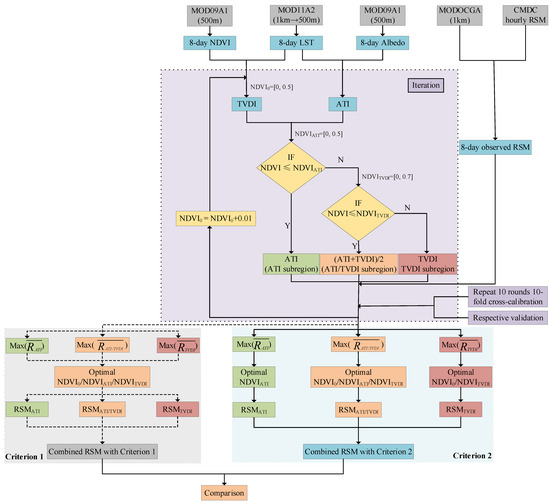
Figure 2.
Flowchart of relative soil moisture (RSM) estimation by the apparent thermal inertia (ATI)-based models, the ATI/TVDI—temperature vegetation dryness index joint models, and the TVDI-based models with Criterion 2 (adapted from [35]). NDVI0 was used for computing TVDI, and both NDVIATI and NDVITVDI were applied for dividing the entire Chinese Loess Plateau (CLP). The three subregions, namely the ATI subregion (NDVI ≤ NDVIATI), the ATI/TVDI subregion (NDVIATI < NDVI ≤ NDVITVDI), and the TVDI subregion (NDVI > NDVITVDI), were assigned by calculated ATI, the average of ATI and TVDI, and TVDI, respectively.
To estimate RSM, the whole CLP was divided into three subregions (the ATI subregion, the TVDI subregion, and the ATI/TVDI subregion) according to the NDVI of individual pixels. While the ATI-based models (ATI) were merely applied to the ATI subregion (NDVI ≤ NDVIATI), the TVDI-based models (TVDI) were merely applied to the TVDI subregion (NDVI > NDVITVDI). Then, the ATI-based models and the TVDI-based models together (the ATI/TVDI joint models—the average of ATI and TVDI) were applied to the ATI/TVDI subregion (NDVIATI < NDVI ≤ NDVITVDI). Here, as mentioned before, the ATI-based model is routinely used to estimate the RSM of bare soil and sparsely vegetated areas with low NDVI and the TVDI-based model is more suitable for dense vegetation coverage with high NDVI. Thus, the case of NDVIATI greater than NDVITVDI is not considered in an individual subregion.
The RSM estimation using the ATI-based, the TVDI-based, and the ATI/TVDI joint models should contain two key procedures. One is the iteration procedure applying three NDVI thresholds to calculate . The other is the identification of optimal NDVI thresholds for subregional RSM estimation. In this study, we proposed a new method to select optimal NDVI thresholds for improving RSM estimation involving increased accuracy and spatiotemporal coverage, which was defined as Criterion 2. Both Criterion 1 and Criterion 2 shared similar iteration procedures (with different maximum iterations) to obtain .
In addition, the NDVI threshold (NDVI0), the lower limit of NDVI, below which the data are excluded when we derive dry/wet edges, would be used for generating TVDI [35]. To obtain optimal NDVI thresholds, NDVI0 and NDVIATI, both ranging from 0 to 0.5, and NDVITVDI, ranging from 0 to 0.7 with an interval of 0.01, were successively tested in the iterative process (Figure 2). We carried out NDVI ranges of the iteration in the programing design used for loops statement and it was easy to run programming using the fixed large range for each 8-day period in 2017. For one iteration, linear relation analysis between an assigned value (e.g., ATI) and the corresponding in situ RSM observations was performed through the 10-fold cross-calibration in the calibration process. Detailed calibration and validation processes are presented in Section 3.2.2. After the completion of all iterations, three groups of optimal NDVI thresholds with a maximum in validation were selected with Criterion 2 for one 8-day period rather than one group with Criterion 1. The overall 8-day RSM map was ultimately produced with the generated subregional RSM by applying the selected optimal thresholds. The comparison between the two criteria was conducted as follows.
3.1.1. Apparent Thermal Inertia (ATI)
Soil TI—thermal inertia is a thermal property of soil and describes the resistance of soil to temperature variations. TI proportionally increases as SM increases because moist soil has higher water thermal conductivity and heat capacity, thereby exhibiting a lower diurnal temperature fluctuation [27,29]. ATI—apparent thermal inertia is a simplified calculation for TI [28,41]. As one of the SM estimation methods, ATI can be easily calculated by measuring surface albedo and the diurnal temperature range as follows:
where is the apparent thermal inertia [K−1], is the broadband surface albedo, and corresponds to the diurnal temperature range between day and night [K]. Theoretically, the MODIS-derived ATI was computed as the ratio of the daily surface albedo and the diurnal temperature range [42]. However, the availability of the MODIS-derived ATI on some days was mainly limited by the availability of satellite LST observations because LST was often absent due to the presence of cloud during the satellite overpass times. Thus, it was difficult to obtain a continuous time series of ATI. In detail, the merged Terra 8-day surface reflectance and temperature products (MOD09A1/MOD11A2) are distributed on 8-day synthesis periods of clear sky data accumulation and each 8-day composite pixel contains the best possible observation according to specified criteria [43]. In addition, previous studies applied MOD11A2 LST products and MOD09A1 surface reflectance data (time resolution of 8 days) to Equation (1) [15,34,44]. In this case, our study was also carried out for an 8-day temporal resolution to calculate ATI. ATI varies between 0 and 1. The broadband albedo can be computed in shortwave spectral ranges from Terra MODIS surface reflectance [45]:
where – and are the reflectance of bands 1, 2, 3, 4, 5, and 7 of MODIS, respectively [15,42,46,47]. MODIS’s six bands are excellent in making the broadband albedo conversions under the general atmospheric conditions [45].
3.1.2. Temperature Vegetation Dryness Index (TVDI)
As the scatter plot of NDVI against LST forms a triangle or trapezium (hereinafter called triangle), Sandholt et al. [48] proposed the concept of TVDI, which can represent RSM, which is formulated as follows:
where LST represents the MODIS-derived LST in each of the pixels, LSTmin and LSTmax refer to the minimum/maximum LST in the triangle space defining the wet/dry edge at a given NDVI, respectively. , , and are the linear regression parameters (slope and intercept) of dry/wet edges, respectively. Based on TVDI, RSM can be related to LSTmin and LSTmax with the following equation [49,50]:
From Equation (6) RSM can be found as:
where RSM is the relative soil moisture at any given pixel, is the maximum RSM according to wet edge, and is the minimum RSM corresponding to dry edge. The trend line of gives the dry edge and that of the represents the wet edge. The NDVI-LST triangle space defining the dry/wet edges on DOY—day of the year 113 over the CLP is shown in Figure 3.

Figure 3.
The NDVI-LST triangle space defining the dry/wet edges on DOY—day of the year 113 over the CLP (adapted from [35,48,51]). Theoretically, in the triangular figure (pink region area), the base edge of the triangle with maximum evapotranspiration pixels, and the top edge of the triangle with zero evapotranspiration pixels are displayed. As the NDVI increases, the maximum LST decreases and can be fitted to a negative slope using the least square method, which is defined as the dry edge in red color lines (LSTmax). The base line of the triangle represents the wet edge in blue color lines (LSTmin), which is calculated by averaging a group of points in the lower limits of the scatterplot. The TVDI increases from 0 to 1 (a black arrow going from TVDI = 0 to TVDI = 1), indicating a land surface change from extreme wetness to extreme drought. Linear equations were generated when NDVI0 equals 0, 0.1, and 0.2, respectively. The linear regression coefficients (slopes, intercepts, and R2) of dry/wet edges varied with different NDVI0.
Generally, the TVDI value of the dry edge, referring to the driest region of the study area, equals 1, while that of the wet edge (being the most humid region) is close to 0 [52]. LST linearly changes with NDVI in the conditions of the same RSM. Between two edges (dry/wet edges), all intermediate conditions can occur, and all RSM conditions can consequently be represented within the NDVI-LST triangle space [31,53]. However, the maximum and minimum LST at lower NDVI in the scatterplot (two red circles in Figure 3) do not seem to contribute to the formation of the dry/wet edges, which has been noted by previous studies [54,55,56]. Thus, in our study, the NDVI0 is the low limit of NDVI, below which the data are excluded when we derive dry/wet edges. The TVDI (NDVI < NDVI0) with Criterion 2 was calculated using the linear regression parameters of derived dry/wet edges, and the TVDI (NDVI < NDVI0) was not computed because of setting NDVI0 smaller than NDVIATI for Criterion 1. In other words, TVDI would only be used both in the ATI/TVDI subregion and the TVDI subregion, where NDVI was higher than NDVIATI, not to mention NDVI0.
3.1.3. RSM Estimation with Criterion 2
The overall RSM was produced with three groups of selected optimal NDVI thresholds (Criterion 2) using MODIS-derived ATI, TVDI, and the mean of ATI and TVDI against in situ RSM observations for one 8-day period. The equations were used as follows:
where represents the overall RSM and it is combined by three subregional RSM (, and ). and are the RSM estimated by the ATI-based and TVDI-based models, respectively, and is the RSM estimated by the ATI/TVDI joint model. and are coefficients from fitting the ATI values and in situ RSM observations in the ATI subregion. and are coefficients from fitting the TVDI values and in situ RSM observations in the TVDI subregion. and are coefficients from fitting the average value of ATI and TVDI and in situ RSM observations in the ATI/TVDI subregion. and are the selected optimal thresholds for generating subregions.
3.2. Comparison of the Two Criteria
3.2.1. Calibration and Validation Processes for the Two Criteria
The two criteria differ in how the optimal NDVI thresholds are identified, namely NDVI0 ≤ NDVIATI ≤ NDVITVDI for Criterion 1 and NDVIATI < NDVITVDI for Criterion 2. In other words, the limit condition of Criterion 1 was stricter than Criterion 2 and the value of NDVI0 might be greater/lower than NDVIATI for Criterion 2. As we mentioned in Section 3.1.2., dry/wet edges were calculated when NDVI was greater than NDVI0. In this case, the value of TVDI (NDVI < NDVI0) was calculated based on the dry/wet edge derived from NDVI greater than NDVI0. The size relationship between NDVI0 and NDVIATI is the main difference of the two criteria, which directly lead to a different assigned value in the ATI/TVDI subregion, thereby affecting the calibration process when using the ATI/TVDI joint models. The detailed differences between subregional RSM estimation with each criterion are represented in Figure 4 and Figure 5. For Criterion 2, the average of ATI and TVDI was assigned to the pixels in the ATI/TVDI subregion, in which TVDI includes two intervals (NDVIATI < NDVI < NDVI0 and NDVI0 ≤ NDVI ≤ NDVITVDI) with Criterion 2 (Figure 5). TVDI with Criterion 1 is from only one interval, namely NDVIATI < NDVI ≤ NDVITVDI in the ATI/TVDI subregion from Figure 4.
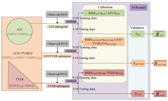
Figure 4.
Schematic diagram of the calibration and validation processes with Criterion 1 (NDVI0 ≤ NDVIATI ≤ NDVITVDI). NDVIATI and NDVITVDI were applied to divide the whole CLP. NDVI0 was lower than NDVIATI and merely used for calculating TVDI (not shown in the figure). ATI, the average of ATI and TVDI, and TVDI were assigned to the ATI subregion (NDVI ≤ NDVIATI), the ATI/TVDI subregion (NDVIATI < NDVI ≤ NDVITVDI), and the TVDI subregion (NDVI > NDVITVDI), respectively. RSMATI and RSMTVDI were the RSM estimated by the ATI-based and TVDI-based models, respectively, and RSMATI/TVDI was the RSM estimated by the ATI/TVDI joint model. aATI, bATI, aTVDI, and bTVDI in the equations were coefficients from fitting the ATI values and TVDI values with in situ RSM observations in the ATI subregion and the TVDI subregion, respectively. aATI/TVDI and bATI/TVDI were coefficients from fitting the average value of ATI and TVDI and in situ RSM observations in the ATI/TVDI subregion. After 10 rounds 10-fold cross-calibration, , , and in validation were calculated by averaging RATI, RATI/TVDI, and RTVDI, respectively.

Figure 5.
Schematic diagram of the calibration and validation processes with Criterion 2 (NDVIATI < NDVITVDI). NDVIATI and NDVITVDI were applied to divide the whole CLP. NDVI0 might be lower/greater than NDVIATI and appeared when NDVI0 was greater than NDVIATI, indicating the calculated TVDI from two NDVI intervals (blue and light orange color regions) in the ATI/TVDI subregion. The value of TVDI with Criterion 2 in the blue color regions (NDVI < NDVI0) was calculated based on the dry/wet edge derived from NDVI greater than NDVI0. The computed TVDI with Criterion 2 in the light orange color regions (NDVI ≥ NDVI0) was the same as that of Criterion 1 (orange color regions in Figure 4). For the meaning of the other parameters (RSMATI, RSMTVDI, RSMATI/TVDI, RATI, RATI/TVDI, RTVDI, , , and ), please refer to the caption of Figure 4.
Importantly, because optimal NDVI thresholds were identified based on the values in the validation, both criteria performed the iteration procedure (calibration and validation processes) in three subregions (the ATI subregion, the TVDI subregion, and the ATI/TVDI subregion) to calculate for 8-day periods (procedures with a purple background in Figure 2). In order to not limit the size of NDVI0 and NDVIATI in the iteration procedure, more iterations would be implemented with Criterion 2 (maximum of 97,546 iterations) than that of Criterion 1 (maximum of 48,620 iterations) [35]. The number of iterations was calculated by all combinations of the three thresholds.
For each subregion, to decrease the variability of the calibration, the linear fit between the assigned value (ATI, the average of ATI and TVDI, and TVDI, respectively) and observed RSM was performed using 10 rounds of 10-fold cross-calibration. To be more specific, after the random splitting of the paired assigned values and in situ RSM observations (when the number of available RSM observation stations was greater than 20) into 10 subsamples with nine as training data and one as testing data, acquired regression parameters (slopes and intercepts) in training data were applied to testing data. Then, one group of estimated RSM and in situ RSM observations was generated. After the 10th fold was accomplished, the validation data of 10 groups of estimated RSM and in situ RSM observations were computed, including R, as well as the p-value for a significance test (p-value < 0.05), which was just called “one-round”. After 10 rounds of iterations, we averaged the R () from the 10 rounds of validation as the reference to identify corresponding optimal NDVI thresholds.
3.2.2. Evaluation of Estimated RSM for the Two Criteria
The threshold qualification when identifying optimal NDVI thresholds for the two criteria was different, but both were based on the averaged validation results (), which directly represents the accuracy of RSM estimation. For an individual subregion, only the maximum greater than 0.23 for Criterion 2 and slightly lower (0.17) for Criterion 1 should be selected; otherwise, no optimal NDVI thresholds were chosen for that subregion. For Criterion 1, the NDVI thresholds corresponding to maximum among the three subregions were chosen as the optimal thresholds when the NDVI0, NDVIATI, and NDVITVDI thresholds existed simultaneously for one 8-day period [35]. In this way, they could not guarantee that maximum would be reached for all the three subregions and the generated three subregions according to NDVIATI and NDVITVDI always excluding each other. Thus, only one group of optimal NDVI thresholds were chosen for subregional RSM estimation and then the overall RSM with Criterion 1 was combined by subregional RSM for each 8-day period [35].
However, for Criterion 2, more selected processes for optimal NDVI thresholds were carried out. The NDVI thresholds corresponding to maximum in each subregion, namely the highest , , and , were chosen as the optimal thresholds. The optimal NDVI thresholds of the three subregions were not influenced by each other. Thus, three groups of optimal NDVI thresholds regarding three subregions were selected for subregional RSM estimation and then the overall RSM with Criterion 2 was combined by that subregional RSM for each 8-day period. In this case, the three subregions for one 8-day period might be overlapped due to the three groups of optimal NDVI thresholds individually selected instead of always excluding each other for Criterion 1. Based on the relationships of the selected optimal NDVI thresholds of the subregions, we list all cases in terms of different combinations of models used to produce an overall RSM map for one 8-day period (Table 1). Overlaps might exist when combining different models for RSM estimation for one 8-day period (see cases 4, 5, 6, and 7 in Table 1).

Table 1.
Cases of the model used with the relationships of selected optimal NDVI thresholds with Criterion 2.
We combined the subregional RSM generated using the corresponding models with the selected optimal NDVI thresholds to obtain an overall RSM map for one 8-day period. Then, we evaluated and compared the selected optimal NDVI thresholds with each criterion in terms of the validation outcomes (Figure 6). Furthermore, the performance of the selected optimal NDVI thresholds for RSM retrieval, involving accuracy and spatiotemporal coverage using the two criteria, was compared. Monthly, seasonal, and yearly RSM maps were generated by combining 8-day RSM maps under Criterion 2 and were eventually examined.
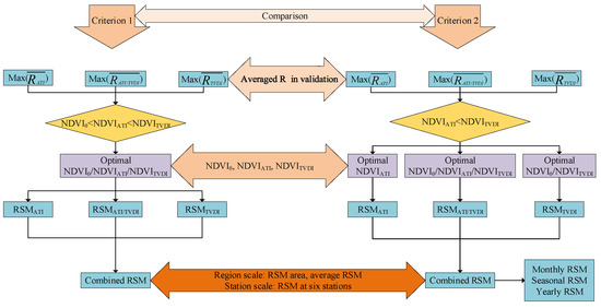
Figure 6.
Flowchart for comparison of the two criteria.
4. Results and Discussion
4.1. Evaluation of the Optimal NDVI Thresholds
4.1.1. Comparison of Validation Results
The measure in validation reflects the accuracy of the estimated RSM compared to the observed RSM. Lower represents poorer estimated RSM. Optimal NDVI thresholds were identified corresponding to the highest in subregions. Then, RSM maps could be generated using the selected optimal NDVI thresholds for each 8-day period. Eventually, we selected 45 8-day periods (out of 46 except for DOY 73 in 2017) with Criterion 2 and only 38 8-day periods with Criterion 1 (Figure 7) [35]. Thus, 45 8-day periods of estimated RSM maps (improved 7 8-day periods compared to with Criterion 1) would be generated with Criterion 2. The values with Criterion 2 were slightly higher than those with Criterion 1 but roughly showed a similar trend throughout the year. These values fluctuated irregularly with peak values (0.82±0.007 with Criterion 2 and 0.75±0.008 with Criterion 1, respectively) in winter [35]. In this case, the accuracy of RSM estimation with Criterion 2 was improved.
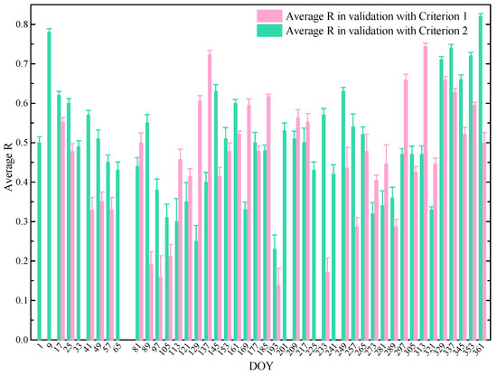
Figure 7.
Comparison of in validation with Criteria 1 and 2. The standard deviation of for each 8-day period is displayed as error bars (one standard deviation). Maximum in validation less than 0.17 and 0.23 for an individual subregion was not selected with Criterion 1 and Criterion 2, respectively. No optimal NDVI thresholds were selected with Criterion 1 on DOYs 1, 9, 33, 65, 73, 201, 225, and 241, resulting in no estimated RSM maps (missed pink bars). Only the 8-day period of DOY 73 with Criterion 2 could not satisfy the minimum standard (0.23).
The applied models corresponding to the highest varied with the 8-day periods. Table 2 displays the validation results as well as the models used for each 8-day period with Criterion 2. The seven rows in blue (DOYs 1, 9, 33, 65, 201, 225, and 241) indicate the new validation results with Criterion 2 for RSM retrieval compared to Criterion 1. The ATI/TVDI joint models were used in almost all 8-day periods (34/45 8-day periods), which was well in line with Criterion 1 [35]. The highest (0.82 ± 0.007 on DOY 361) with Criterion 2 was higher than that of Criterion 1 (0.75 ± 0.008 on DOY 313). The validation score of was better than previous results in the study area [35].
Table 2.
Validation results for selecting optimal NDVI thresholds with Criterion 2 (blue color rows represent new 8-day periods of validation results compared to Criterion 1).
For DOYs 145 and 305, the ATI/TVDI joint models were applied twice in the two complementary ATI/TVDI subregions with different NDVI ranges (0.00 < NDVI ≤ 0.20 with of 0.61 ± 0.044 and 0.25 < NVDI ≤ 0.27 with of 0.63±0.017 on DOY 145, and 0.13 < NDVI ≤ 0.17 with of 0.47 ± 0.021 and 0.30 < NDVI ≤ 0.34 with of 0.44 ± 0.020 on DOY 305, respectively). In the ATI/TVDI subregions, different NDVI thresholds (NDVIATI and NDVITVDI) means the generated RSM maps with these NDVI intervals. Here, higher , not merely the highest , could be selected as well and their corresponding thresholds were regarded as additional thresholds for RSM retrieval. In this context, the two complementary ATI/TVDI subregional RSM could be merged to produce the overall RSM map. Thus, the more additional thresholds we selected, the more completed the obtained RSM map would be. The additional NDVI thresholds we applied, here, was another improved strategy to acquire wider coverage of RSM estimation. The number of stations used with each criterion was the same for each 8-day period.
4.1.2. The Optimal NDVI Thresholds
The thresholds NDVIATI and NDVITVDI were used to divide the entire study area into three subregions for subregional RSM estimation. In terms of the fixed ranges of NDVI0, NDVIATI, and NDVITVDI we used during iteration, to cover more combinations of NDVI thresholds, the variation of NDVI for all seasons was taken into consideration and maximum possible ranges were selected throughout the year. Indeed, the NDVI ranges we used were a little bit wide compared to other studies, to some extent, resulting in many redundant iterations [33,40]. There was no significant trend in these optimal thresholds throughout the year. It would be explained by taking into account seasonal change (or phenological variation) effects on prediction. To better explain the variation of the NDVI threshold, the construction of seasonal models should be considered over long periods for further studies. Moreover, the NDVI threshold could improve the application of other phenology-based RSM estimation methods meant basically for the growing season [58,59,60].
The selected minimum and maximum NDVIATI (0.00 and 0.50) and NDVITVDI (0.09 and 0.68) are shown in Table 2. The obvious difference between the two criteria was the identification of NDVI0, which not only determines the value of TVDI but also affects the value of pixels in the ATI/TVDI subregion. The pixels with NDVIATI < NDVI ≤ NDVITVDI were assigned the average of ATI and TVDI in the ATI/TVDI subregion for two criteria, but some of the TVDI (NDVIATI < NDVI < NDVI0) were calculated by the wet/dry edges produced from those NDVI higher than NDVI0 for Criterion 2. The identification of NDVIATI was not affected by the other two thresholds with Criterion 2 and the biggest NDVIATI was 0.50 solely using the ATI-based models on DOY 201. The selected NDVITVDI with Criterion 2 was up to 0.68, approaching the upper limited value (0.70) on DOY 81 using the ATI/TVDI joint models.
In terms of NDVI0 for the NDVI–LST scatter plots, the value of selected NDVI0 with Criterion 2 fluctuated over 8-day periods but remained relatively low and stable in winter (DOYs 1–49 and 337–361). Most of were higher than , particularly in summer (DOYs 153–233), and peaked in spring and autumn (Figure 8b). The slopes (adry and awet) and intercepts (bdry and bwet) of the regression equations changed symmetrically (Figure 8a) and showed similar trends regardless of the criterion [35].
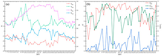
Figure 8.
The parameters of the dry and wet edges for 8-day periods in 2017: (a) Slopes and intercepts corresponding to selected NDVI0: adry, awet, bdry, and bwet; (b) correlation coefficients with selected NDVI0: and .
4.2. Comparison of Estimated RSM
4.2.1. Evaluation of Estimated RSM at the Regional Scale
The estimated RSM area and average RSM obtained with each of the two criteria varied throughout the year (Figure 9). There were 45 8-day periods of the RSM maps produced in 2017 with Criterion 2, compared to 38 with Criterion 1 [35]. This clearly shows that using Criterion 2 improved the temporal coverage of RSM estimation.
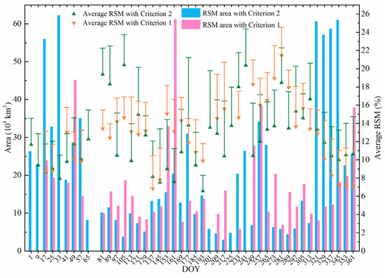
Figure 9.
Comparison of the estimated RSM area and of the average RSM with each criterion. The standard deviation of RSM of all pixels for each 8-day period is shown as error bars (one standard deviation).
In terms of spatial coverage, the two criteria also led to different RSM estimation results. The total area of estimated RSM with Criterion 2 was 939.52 × 10⁴ km2 in 2017, which was 40.76% higher than with Criterion 1 (667.44 × 10⁴ km2). Among the 45 8-day periods, there were 24 8-day periods for which Criterion 2 produced a larger geographical area of estimated RSM than Criterion 1. The increased area of estimated RSM ranged from 0.30 × 10⁴ km2 on DOY 81 to 52.58 × 10⁴ km2 on DOY 321 and the average increased area was 19.77 × 10⁴ km2 [35]. Therefore, RSM estimation with Criterion 2 also improved the spatial coverage compared with Criterion 1.
Despite such differences in spatiotemporal coverage, estimated RSM with each criterion also shared some similarities. Both average RSM were highest (~22%) in autumn (DOYs 241–329), which agrees with the study by Jiao et al. (2016) that reported autumn had higher average SM than other seasons in 1998–2000 over the CLP [61]. In addition, we also found that spring (DOYs 57–145) had higher RSM than winter (DOYs 1–49 and 337–361) and summer (DOYs 153–233) (Figure 9).
It should be noted that the area produced by Criterion 1 could occasionally be greater than that of Criterion 2 (e.g., DOYs 49, 105, 153, 161, 249, and 289). The used optimal NDVIATI, NDVITVDI, in validation, and estimated RSM area with each criterion for these 8-day periods are shown in Table 3. Models performed better with Criterion 2 (higher in validation) despite a greater estimated RSM area with Criterion 1. Thus, we could not conclude that Criterion 1 was better than Criterion 2 by merely considering the spatial coverage. In addition, as we mentioned in Section 4.1.1, to acquire wider coverage of RSM estimation, we could choose the additional NDVI thresholds to estimate RSM, which corresponds to higher rather than the highest . Therefore, we might test more additional NDVI thresholds in subregions to combine the overall RSM map with the desired accuracy for further study.
Table 3.
Comparison selected optimal NDVIATI, NDVITVDI, , and estimated RSM area of two criteria (area produced by Criterion 1 was greater than that of Criterion 2). Models that performed better for 8-day periods are in bold.
4.2.2. Evaluation of Estimated RSM at the Station Scale
At the station scale, in order to reflect the overall result, stations should be uniformly distributed as much as possible with diverse geographical characterization (e.g., precipitation, elevation, and land cover). In addition, stations with more than 23 8-day periods (half of the 46 8-day periods) of estimated RSM could be considered to better reveal the variation of the estimated RSM and the observed RSM. In this case, six stations (station 53,553, station 53,771, station 53,845, station 53,857, station 57,031, and station 57,048) were selected from those stations as samples. The estimated RSM with each criterion and observed RSM with the total 8-day precipitation of six stations (described in Table 4) are presented in Figure 10. A detailed comparison reveals that despite missing some of the estimated RSM, especially for Criterion 1, the values of estimated and observed RSM have the same tendency. Importantly, the estimated RSM (closer to the observation) with Criterion 2 kept a better trend with the observed RSM at the station scale. Moreover, more estimated RSM with Criterion 2 was observed than with Criterion 1 throughout the period among six stations (the blue lines look more consistent than the red lines in Figure 10). The maximum estimated RSM values (near DOY 281) were observed in autumn among the six stations, consistent with heavy rainfall at that time.
Table 4.
Descriptions of the six automatic RSM observation stations.
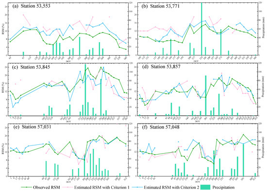
Figure 10.
Comparison of estimated and observed RSM with precipitation at six observation stations in 2017.
With increased precipitation, RSM increased at station 53,553 on DOYs 185, 233, and 281; at station 53,771 on DOYs 169, 209, and 233; at station 53,845 on DOYs 233 and 281; at station 53,857 on DOYs 49 and 241; at station 57,031 on DOYs 97 and 225; and at station 57,048 on DOYs 105 and 265 (Figure 10). In addition, the lag-effect impact of precipitation on RSM reflected at station 53,771 from DOYs 153 to 161 and from DOYs 233 to 241 (less precipitation but higher RSM on DOYs 161 and 241 compared with DOYs 153 and 233, respectively), at station 53,845 from DOYs 233 to 241, at station 57,031 from DOYs 201 to 209, and at station 57,048 from DOYs 201 to 209. The impact of precipitation’s lag-effect on the estimated RSM has been studied [62] and RSM might be increased dramatically after rainfall due to a delayed response of RSM changes to rainfall [13]. Moreover, high estimated RSM was observed in the periods when there were records of rainfall events. Meanwhile, one limitation of this study was that there were some temporal differences between in situ observations and the remote sensing imagery used.
4.3. Evaluation of Estimated RSM with Criterion 2
4.3.1. Estimated Monthly RSM
The maps of monthly estimated RSM via Criterion 2 are demonstrated in Figure 11. The change of color from orange, red, green, and blue represents the gradual increase of RSM. RSM was higher in the southern part of the CLP in winter (December, January, and February), and in the western area in spring (March, April, and May) based on the clustering of the blue color. The soil in autumn (September, October, and November) was generally wetter than other seasons because most of the area was covered by green. The wetter soil might be mainly due to concentrated precipitation in autumn. Obviously, the estimated RSM maps in winter were more complete. Some researchers applied other dryness indices (e.g., PDI) or modified TVDI to estimate RSM [16,33,63,64]. To obtain more complete (monthly) RSM maps, ATI and TVDI could be replaced by other dryness indices to estimate RSM with Criterion 2 in our future research.
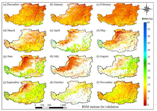
Figure 11.
Spatiotemporal pattern of monthly RSM over the CLP in 2017. The location of available RSM observation stations for validation is displayed on each RSM map. White color over the CLP for each monthly RSM map means no value of RSM calculated with Criterion 2.
Importantly, the number of RSM stations for RSM verification varied among months. The available RSM stations are related not only to observation throughout the month but also to estimation in that month. In this case, there are fewer RSM stations for validation in January and February because of no RSM observations in the frozen soil and in April and October because of relatively incomplete RSM maps, respectively. The maximum station for validation was 180 in November and the minimum station was 59 in January and April (Figure 12). There is a rule of thumb for interpreting the size of the correlation coefficient using the absolute value of the Pearson’s r: 0.00–0.30, very weak; 0.30–0.50, weak; 0.50–0.70, moderate; 0.70–0.90, strong; and 0.90–1.00, very strong [65,66]. Estimated RSM had a weak correlation with the observed RSM in most months and the highest Pearson’s r was 0.68 in January. The root mean square error (RMSE) varied from 3.77% in April to 6.10% in October. The highest mean absolute error (MAE) also appeared in October (4.97%) and the lowest MAE was 3.02% in March.
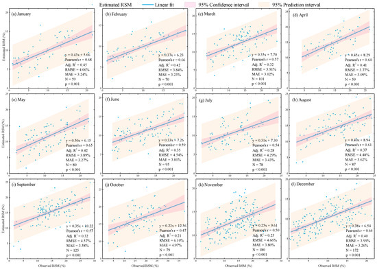
Figure 12.
Scatter plots of the observed and estimated RSM at the monthly time scale (linear fitting shown by blue lines with 95% confidence interval and 95% prediction interval shaded in pink and orange, respectively). Scores (Pearson’s correlation coefficient (Pearson’s r), adjusted R2, root mean square error (RMSE), and mean absolute error (MAE)) were computed using data included in the corresponding subplot boundary. N represents the number of available RSM observation station samples for each month. The associated p-values (p in the subplots) with the correlation coefficients are <0.001.
The estimated monthly RSM and their area is illustrated in Figure 13. The average RSM varied from 8.64% in February to 16.42% in August and the highest and lowest maximum RSM (60.96% and 20.93%) appeared in September and January, respectively. The minimum RSM value was 0.00% for most months. However, there were two peaks in spring and the average RSM was clustered in the peak valley (11.42% in March, 14.18% in April, and 10.50% in May, respectively). The total area of the generated RSM area in February was the greatest (62.39 × 10⁴ km2). The area of generated RSM in April, July, and October was quite small (less than half the area of the CLP). Through comparison of the area distribution of the estimated RSM to the frequency of the observed RSM at available stations, similar tendencies were demonstrated for most months except in January and February. This might be attributed to the scarce RSM observations at that time, thus failing to reflect the spatial distribution of the whole CLP.
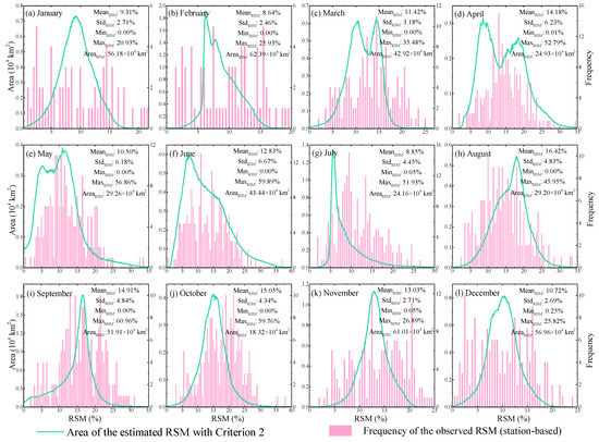
Figure 13.
The plots of monthly RSM with its area and frequency of the observed RSM (station-based) in 2017. The average RSM (MeanRSM), standard deviation (StdRSM) of RSM, minimum RSM (MinRSM), maximum RSM (MaxRSM) of all pixels, and the area of the generated RSM were computed monthly.
4.3.2. Estimated Seasonal and Yearly RSM
The seasonal and yearly RSM maps with the statistics of RSM are shown in Figure 14. Although estimated RSM had a weak correlation with the observed RSM among seasons (Pearson’s r ranges from 0.53 in spring to 0.67 in winter and autumn), there was a moderate correlation (0.73) for annual RSM. RMSE varied from 3.74% in winter to 4.41% in autumn. The highest MAE also appeared in autumn (3.64%) and the lowest MAE was 3.00% for annual RSM. We found that autumn had the greatest error among the four seasons, which was highly related to the corresponding months (September, October, and November) with the higher error of RSM estimation (Figure 12). In addition, the generated RSM area of these months in autumn was small and the merged seasonal RSM map would also have a larger error because the seasonal RSM of a certain pixel might be computed by the estimated RSM of a specific month instead of all months in autumn.
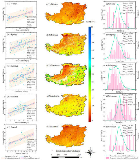
Figure 14.
Seasonal and yearly RSM: (a1–e1) Scatter plots of the observed and estimated RSM at a seasonal and yearly time scale (linear fitting shown by blue lines with 95% confidence interval and 95% prediction interval shaded in pink and orange, respectively). Scores (Pearson’s r, Adjusted R2, RMSE, and MAE) were computed using observed and estimated RSM. N represents the number of available RSM observation station samples for each period. The associated p-values with the correlation coefficients are <0.001; (a2–e2) spatiotemporal pattern of seasonal and yearly RSM over the CLP in 2017. The location of available RSM observation stations for validation is displayed on each RSM map. The white color of seasonal and yearly maps over the CLP means no value of RSM calculated with Criterion 2; (a3–e3) the plots of seasonal and yearly RSM with its area and frequency of the observed RSM (station-based) in 2017. The average RSM (MeanRSM), standard deviation (StdRSM) of RSM, minimum RSM (MinRSM), and maximum RSM (MaxRSM) of all pixels and the area of the generated RSM were computed.
The available RSM stations for validation were 49 in the year 2017, which means only 49 observation stations have continuous RSM observations throughout the year. Meanwhile, the scarce RSM observations in winter and 2017 could not reflect the spatial distribution of the estimated RSM for the whole CLP (Figure 14(a3,e3)). The seasonal difference of RSM over the CLP is distinct in 1998–2000 and 2008–2010 [61], which agrees with our results especially for summer (dryer in the southeastern area and wetter in the remaining regions). The southeastern regions were affected by drought and extreme drought after analyzing the drought variation trends in different subregions of the CLP over four decades [67]. However, mean RSM was highest in autumn and lowest in spring [61], which is slightly different from our results (highest (13.91%) in autumn but lowest (9.08%) in winter). The reason for such a difference might be that they just compared SM in three seasons (spring, summer, and autumn) while we evaluated all four seasons [61].
5. Conclusions
This study aimed to improve the relative soil moisture (RSM) estimation that is based on the apparent thermal inertia (ATI) and temperature vegetation dryness index (TVDI). By optimizing the identification of NDVI thresholds, Criterion 2 (NDVIATI<NDVITVDI) improved both the accuracy and spatiotemporal coverage of estimation compared with Criterion 1 (NDVI0 ≤ NDVIATI ≤ NDVITVDI). In addition, monthly, seasonal, and yearly RSM maps of the Chinese Loess Plateau (CLP) in 2017 were produced via the 8-day RSM maps and then examined. From our results, we conclude that:
- The ATI/TVDI joint models not only have higher applicability than the ATI-based and TVDI-based models for all 8-day periods but also for simultaneous use within different NDVI ranges in the ATI/TVDI subregions for one 8-day period. Thus, in addition to the optimal NDVI thresholds, the additional NDVI thresholds we applied was another improved strategy to acquire wider spatial coverage of RSM estimation.
- NDVI thresholds were optimized for robust RSM estimation with Criterion 2 for each 8-day period over the CLP and the selected optimal thresholds constantly changed throughout the study period. The applicability of Criterion 2, involving spatiotemporal coverage (45 and 38 8-day periods of RSM maps and the total RSM area of 939.52 × 10⁴ km2 and 667.44 × 10⁴ km2 with Criterion 2 and Criterion 1, respectively) and the accuracy (maximum of 0.82 ± 0.007 for Criterion 2 and of 0.75 ± 0.008 for Criterion 1) of estimated RSM, was better than that of Criterion 1.
- The estimated RSM (closer to the observation) with Criterion 2 kept a better trend with the observed RSM at the station scale. Moreover, more estimated RSM with Criterion 2 was observed than with Criterion 1 throughout the period.
- High estimated RSM was observed in the periods when there were records of rainfall events, especially in autumn (mean RSM of 13.91 ± 2.65%)—wetter than other seasons. With a mean annual RSM of 10.16 ± 2.21%, the annual RSM map shows dryer areas in the southeastern part of the CLP.
This study focused on improving RSM estimation from MODIS imagery with Criterion 2, and such effort is still fundamental to the general research of SM remote sensing. We improved the mapping of RSM using Criterion 2. The next steps following this research would extend the retrieval to other sensors like Landsat and Sentinel satellites, to perform reliable estimates of SM at a high spatiotemporal resolution.
Author Contributions
Conceptualization, L.Y. (Lina Yuan) and L.L.; methodology, L.Y. (Lina Yuan); software, W.L. and S.H.; validation, L.Y. (Lina Yuan) and J.Z.; resources, T.Z., L.Y. (Longhua Yang) and L.C. (Liang Cheng); writing—original draft preparation, L.Y. (Lina Yuan) and T.Z.; writing—review and editing, L.L. and L.C. (Longqian Chen); visualization, M.W. and W.L.; supervision, L.C. (Longqian Chen) and L.L. All authors have read and agreed to the published version of the manuscript.
Funding
This research was supported by the Fundamental Research Funds for the Central Universities (Grant No.: 2018ZDPY07).
Institutional Review Board Statement
Not applicable for this study.
Informed Consent Statement
Not applicable for this study.
Data Availability Statement
The input data used in this research can be accessed freely from online sources.
Acknowledgments
The authors would like to thank the China Meteorological Data Service Center (CMDC, http://data.cma.cn/) for providing in situ RSM observations data over the CLP. Remote sensing data were freely provided by the NASA Land Processes Distributed Active Archive Center (LP DAAC, https://lpdaac.usgs.gov/). Furthermore, we appreciate the editors and reviewers for their constructive comments and suggestions.
Conflicts of Interest
The authors declare no conflict of interest.
References
- Kumar, S.V.; Dirmeyer, P.A.; Peters-Lidard, C.D.; Bindlish, R.; Bolten, J. Information Theoretic Evaluation of Satellite Soil Moisture Retrievals. Remote Sens. Environ. 2018, 204, 392–400. [Google Scholar] [CrossRef]
- Li, Z.; Lin, X.; Coles, A.E.; Chen, X. Catchment-Scale Surface Water-Groundwater Connectivity on China’s Loess Plateau. Catena 2017, 152, 268–276. [Google Scholar] [CrossRef]
- Hou, J.; Zhu, H.; Fu, B.; Lu, Y.; Zhou, J. Functional Traits Explain Seasonal Variation Effects of Plant Communities on Soil Erosion in Semiarid Grasslands in the Loess Plateau of China. Catena 2020, 194, 104743. [Google Scholar] [CrossRef]
- Zhao, J.; Van Oost, K.; Chen, L.; Govers, G. Moderate Topsoil Erosion Rates Constrain the Magnitude of the Erosion-Induced Carbon Sink and Agricultural Productivity Losses on the Chinese Loess Plateau. Biogeosciences 2016, 13, 4735–4750. [Google Scholar] [CrossRef]
- Djamai, N.; Magagi, R.; Goïta, K.; Merlin, O.; Kerr, Y.; Roy, A. A Combination of DISPATCH Downscaling Algorithm with CLASS Land Surface Scheme for Soil Moisture Estimation at Fine Scale during Cloudy Days. Remote Sens. Environ. 2016, 184, 1–14. [Google Scholar] [CrossRef]
- Hardy, A.J.; Barr, S.L.; Mills, J.P.; Miller, P.E. Characterising Soil Moisture in Transport Corridor Environments Using Airborne LIDAR and CASI data. Hydrol. Process. 2011, 26, 1925–1936. [Google Scholar] [CrossRef]
- Yee, M.S.; Walker, J.P.; Rüdiger, C.; Parinussa, R.M.; Koike, T.; Kerr, Y.H. A Comparison of SMOS and AMSR2 Soil Moisture Using Representative Sites of the OzNet Monitoring Network. Remote Sens. Environ. 2017, 195, 297–312. [Google Scholar] [CrossRef]
- Zawadzki, J.; Kedzior, M. Soil Moisture Variability over Odra Watershed: Comparison between SMOS and GLDAS Data. Int. J. Appl. Earth Obs. Geoinf. 2016, 45, 110–124. [Google Scholar] [CrossRef]
- Ebrahimi-Khusfi, M.; Alavipanah, S.K.; Hamzeh, S.; Amiraslani, F.; Samany, N.N.; Wigneron, J.-P. Comparison of Soil Moisture Retrieval Algorithms Based on the Synergy Between SMAP and SMOS-IC. Int. J. Appl. Earth Obs. Geoinf. 2018, 67, 148–160. [Google Scholar] [CrossRef]
- Escorihuela, M.J.; Quintana-Seguí, P. Comparison of Remote Sensing and Simulated Soil Moisture Datasets in Mediterranean Landscapes. Remote Sens. Environ. 2016, 180, 99–114. [Google Scholar] [CrossRef]
- Pardé, M.; Wigneron, J.-P.; Chanzy, A.; Waldteufel, P.; Kerr, Y.; Huet, S. Retrieving Surface Soil Moisture over a Wheat Field: Comparison of Different Methods. Remote Sens. Environ. 2003, 87, 334–344. [Google Scholar] [CrossRef]
- Holgate, C.M.; De Jeu, R.; Van Dijk, A.; Liu, Y.; Renzullo, L.; Vinodkumar; Dharssi, I.; Parinussa, R.; Van Der Schalie, R.; Gevaert, A.; et al. Comparison of Remotely Sensed and Modelled Soil Moisture Data Sets across Australia. Remote Sens. Environ. 2016, 186, 479–500. [Google Scholar] [CrossRef]
- Agutu, N.; Awange, J.; Zerihun, A.; Ndehedehe, C.; Kuhn, M.; Fukuda, Y. Assessing Multi-Satellite Remote Sensing, Reanalysis, and Land Surface Models’ Products in Characterizing Agricultural Drought in East Africa. Remote Sens. Environ. 2017, 194, 287–302. [Google Scholar] [CrossRef]
- Hu, T.; Van Dijk, A.I.; Renzullo, L.J.; Xu, Z.; He, J.; Tian, S.; Zhou, J.; Li, H. On Agricultural Drought Monitoring in Australia Using Himawari-8 Geostationary Thermal Infrared Observations. Int. J. Appl. Earth Obs. Geoinf. 2020, 91, 102153. [Google Scholar] [CrossRef]
- Yu, Y.; Wang, J.; Cheng, F.; Chen, Y. Soil Moisture by Remote Sensing Retrieval in the Tropic of Cancer of Yunnan Province. Pol. J. Environ. Stud. 2020, 29, 1981–1993. [Google Scholar] [CrossRef]
- Amani, M.; Salehi, B.; Mahdavi, S.; Masjedi, A.; Dehnavi, S. Temperature-Vegetation-soil Moisture Dryness Index (TVMDI). Remote Sens. Environ. 2017, 197, 1–14. [Google Scholar] [CrossRef]
- Babaeian, E.; Sadeghi, M.; Franz, T.E.; Jones, S.B.; Tuller, M. Mapping Soil Moisture with the OPtical TRApezoid Model (OPTRAM) Based on Long-Term MODIS Observations. Remote Sens. Environ. 2018, 211, 425–440. [Google Scholar] [CrossRef]
- Hashemian, M.; Ryu, D.; Crow, W.T.; Kustas, W.P. Improving Root-Zone Soil Moisture Estimations Using Dynamic Root Growth and Crop Phenology. Adv. Water Resour. 2015, 86, 170–183. [Google Scholar] [CrossRef]
- Rahimzadeh-Bajgiran, P.; Berg, A.A.; Champagne, C.; Omasa, K. Estimation of Soil Moisture Using Optical/Thermal Infrared Remote Sensing in the Canadian Prairies. ISPRS J. Photogramm. Remote Sens. 2013, 83, 94–103. [Google Scholar] [CrossRef]
- Zhang, F.; Zhang, L.-W.; Shi, J.-J.; Huang, J.-F. Soil Moisture Monitoring Based on Land Surface Temperature-Vegetation Index Space Derived from MODIS Data. Pedosphere 2014, 24, 450–460. [Google Scholar] [CrossRef]
- Taktikou, E.; Papaioannou, G.; Bourazanis, G.; Kerkides, P. Soil Moisture Assessment from MODIS data. Desalination Water Treat. 2017, 99, 59–71. [Google Scholar] [CrossRef]
- Phillips, A.J.; Newlands, N.K.; Liang, S.H.; Ellert, B.H. Integrated Sensing of Soil Moisture at the Field-Scale: Measuring, Modeling and Sharing for Improved Agricultural Decision Support. Comput. Electron. Agric. 2014, 107, 73–88. [Google Scholar] [CrossRef]
- Zhang, T.; Wen, J.; Su, Z.; Van Der Velde, R.; Timmermans, J.; Liu, R.; Liu, Y.; Li, Z. Soil Moisture Mapping over the Chinese Loess Plateau Using ENVISAT/ASAR data. Adv. Space Res. 2009, 43, 1111–1117. [Google Scholar] [CrossRef]
- Baghdadi, N.; Zribi, M.; Loumagne, C.; Ansart, P.; Anguela, T. Analysis of TerraSAR-X Data and Their Sensitivity to Soil Surface Parameters over Bare Agricultural Fields. Remote Sens. Environ. 2008, 112, 4370–4379. [Google Scholar] [CrossRef]
- Jin, Y.; Ge, Y.; Wang, J.; Heuvelink, G.B. Deriving Temporally Continuous Soil Moisture Estimations at Fine Resolution by Downscaling Remotely Sensed Product. Int. J. Appl. Earth Obs. Geoinf. 2018, 68, 8–19. [Google Scholar] [CrossRef]
- Mulder, V.; De Bruin, S.; Schaepman, M.; Mayr, T. The Use of Remote Sensing in Soil and Terrain Mapping—A Review. Geoderma 2011, 162, 1–19. [Google Scholar] [CrossRef]
- Van Doninck, J.; Peters, J.; De Baets, B.; De Clercq, E.M.; Ducheyne, E.I.; Verhoest, N.E.C. The Potential of Multitemporal Aqua and Terra MODIS Apparent Thermal Inertia as a Soil Moisture Indicator. Int. J. Appl. Earth Obs. Geoinf. 2011, 13, 934–941. [Google Scholar] [CrossRef]
- Price, J.C. On the Analysis of Thermal Infrared Imagery: The Limited Utility of Apparent Thermal Inertia. Remote. Sens. Environ. 1985, 18, 59–73. [Google Scholar] [CrossRef]
- Taktikou, E.; Bourazanis, G.; Papaioannou, G.; Kerkides, P. Prediction of Soil Moisture from Remote Sensing Data. Procedia Eng. 2016, 162, 309–316. [Google Scholar] [CrossRef][Green Version]
- Lu, L.; Luo, G.-P.; Wang, J.-Y. Development of an ATI-NDVI Method for Estimation of Soil Moisture from MODIS data. Int. J. Remote. Sens. 2014, 35, 3797–3815. [Google Scholar] [CrossRef]
- Rahimzadeh-Bajgiran, P.; Omasa, K.; Shimizu, Y. Comparative Evaluation of the Vegetation Dryness Index (VDI), the Temperature Vegetation Dryness Index (TVDI) and the improved TVDI (iTVDI) for Water Stress Detection in Semi-arid Regions of Iran. ISPRS J. Photogramm. Remote Sens. 2012, 68, 1–12. [Google Scholar] [CrossRef]
- Liu, Y.; Yue, H. The Temperature Vegetation Dryness Index (TVDI) Based on Bi-Parabolic NDVI-Ts Space and Gradient-Based Structural Similarity (GSSIM) for Long-Term Drought Assessment Across Shaanxi Province, China (2000–2016). Remote Sens. 2018, 10, 959. [Google Scholar] [CrossRef]
- Wang, H.; He, N.; Zhao, R.; Ma, X. Soil Water Content Monitoring Using Joint Application of PDI and TVDI Drought Indices. Remote Sens. Lett. 2020, 11, 455–464. [Google Scholar] [CrossRef]
- Lu, X.J.; Zhou, B.; Yan, H.B.; Luo, L.; Huang, Y.H.; Wu, C.L. Remote Sensing Retrieval of Soil Moisture in Guangxi Based on Ati and Tvdi Models. ISPRS—Int. Arch. Photogramm. Remote Sens. Spat. Inf. Sci. 2020, 42, 895–902. [Google Scholar] [CrossRef]
- Yuan, L.; Li, L.; Zhang, T.; Chen, L.; Zhao, J.; Hu, S.; Cheng, L.; Liu, W. Soil Moisture Estimation for the Chinese Loess Plateau using MODIS-derived ATI and TVDI. Remote Sens. 2020, 12, 3040. [Google Scholar] [CrossRef]
- Su, C.; Fu, B. Evolution of Ecosystem Services in the Chinese Loess Plateau under Climatic and Land Use Changes. Glob. Planet. Chang. 2013, 101, 119–128. [Google Scholar] [CrossRef]
- Tasumi, M.; Kimura, R. Estimation of Volumetric Soil Water Content over the Liudaogou River Basin of the Loess Plateau Using the SWEST Method with Spatial and Temporal Variability. Agric. Water Manag. 2013, 118, 22–28. [Google Scholar] [CrossRef]
- Xin, Z.; Yu, X.; Li, Q.; Lu, X.X. Spatiotemporal Variation in Rainfall Erosivity on the Chinese Loess Plateau during the Period 1956–2008. Reg. Environ. Chang. 2010, 11, 149–159. [Google Scholar] [CrossRef]
- McFeeters, S.K. The use of the Normalized Difference Water Index (NDWI) in the Delineation of Open Water Features. Int. J. Remote Sens. 1996, 17, 1425–1432. [Google Scholar] [CrossRef]
- Zhao, J.-P.; Zhang, X.; Bao, H.-Y.; Tong, Q.-X.; Wang, X.-Y.; Liao, C.-H. Monitoring Land Surface Soil Moisture: Co-inversion of Visible, Infrared and Passive Microwave Sensing Data. J. Infrared Millim. Waves 2012, 31, 137–142. [Google Scholar] [CrossRef]
- Claps, P.; LaGuardia, G. Assessing Spatial Variability of Soil Water Content through Thermal Inertia and NDVI. Remote Sens. Agric. Ecosyst. Hydrol. V 2004, 5232, 378–388. [Google Scholar] [CrossRef]
- Pablos, M.; González-Zamora, Á.; Sanchez, N.; Martínez-Fernández, J. Assessment of Root Zone Soil Moisture Estimations from SMAP, SMOS and MODIS Observations. Remote Sens. 2018, 10, 981. [Google Scholar] [CrossRef]
- Vermote, E.F.; Roger, J.C.; Ray, J.P. MODIS Surface Reflectance User’s Guide Collection 6. Available online: http://modis-sr.ltdri.org (accessed on 15 November 2018).
- Qin, J.; Yang, K.; Lu, N.; Chen, Y.; Zhao, L.; Han, M. Spatial Upscaling of in-Situ Soil Moisture Measurements Based on MODIS-Derived Apparent Thermal Inertia. Remote Sens. Environ. 2013, 138, 1–9. [Google Scholar] [CrossRef]
- Liang, S.; Shuey, C.J.; Russ, A.L.; Fang, H.; Chen, M.; Walthall, C.L.; Daughtry, C.S.; Hunt, R. Narrowband to Broadband Conversions of Land Surface Albedo: II. Validation. Remote Sens. Environ. 2003, 84, 25–41. [Google Scholar] [CrossRef]
- Verstraeten, W.W.; Veroustraete, F.; Van Der Sande, C.J.; Grootaers, I.; Feyen, J. Soil Moisture Retrieval Using Thermal Inertia, Determined with Visible and Thermal Spaceborne Data, Validated for European Forests. Remote Sens. Environ. 2006, 101, 299–314. [Google Scholar] [CrossRef]
- Minacapilli, M.; Cammalleri, C.; Ciraolo, G.; D’Asaro, F.; Iovino, M.; Maltese, A. Thermal Inertia Modeling for Soil Surface Water Content Estimation: A Laboratory Experiment. Soil Sci. Soc. Am. J. 2012, 76, 92–100. [Google Scholar] [CrossRef]
- Sandholt, I.; Rasmussen, K.; Andersen, J. A simple interpretation of the surface temperature/vegetation index space for assessment of surface moisture status. Remote Sens. Environ. 2002, 79, 213–224. [Google Scholar] [CrossRef]
- Shen, R.; Yu, P.; Yan, J.; Wang, Y. Retrieving Soil Moisture by TVDI Based on Different Vegetation Index: A Case Study of Shanxi Province. In Proceedings of the International Conference on Computer Science and Electronics Engineering, Hangzhou, China, 23–25 March 2012; pp. 418–422. [Google Scholar] [CrossRef]
- Runping, S.; Jing, Y. Soil Moisture Retrieval through Satellite Data for Gansu and Xinjiang Region of China. Pak. J. Meterorol. 2012, 9, 93–98. [Google Scholar]
- Tagesson, T.; Horion, S.; Nieto, H.; Fornies, V.Z.; González, G.M.; Bulgin, C.; Ghent, D.; Fensholt, R. Disaggregation of SMOS Soil Moisture over West Africa Using the Temperature and Vegetation Dryness Index Based on SEVIRI land Surface Parameters. Remote Sens. Environ. 2018, 206, 424–441. [Google Scholar] [CrossRef]
- Li, H.; Li, C.; Lin, Y.; Lei, Y. Surface Temperature Correction in TVDI to Evaluate Soil Moisture over a Large Area. J. Food Agric. Environ. 2010, 8, 1141–1145. [Google Scholar]
- Holidi, H.; Armanto, M.E.; Damiri, N.; Putranto, D.D.A. Characteristics of Selected Peatland uses and Soil Moisture Based on TVDI. J. Ecol. Eng. 2019, 20, 194–200. [Google Scholar] [CrossRef]
- Chen, J.; Wang, C.; Jiang, H.; Mao, L.; Yu, Z. Estimating Soil Moisture Using Temperature–Vegetation Dryness Index (TVDI) in the Huang-huai-hai (HHH) plain. Int. J. Remote Sens. 2011, 32, 1165–1177. [Google Scholar] [CrossRef]
- Peng, W.; Wang, J.; Zhang, J.; Zhang, Y. Soil Moisture Estimation in the Transition Zone from the Chengdu Plain Region to the Longmen Mountains by Field Measurements and LANDSAT 8 OLI/TIRS-Derived Indices. Arab. J. Geosci. 2020, 13, 1–13. [Google Scholar] [CrossRef]
- Yang, R.; Wang, H.; Hu, J.; Cao, J.; Yang, Y. An Improved Temperature Vegetation Dryness Index (iTVDI) and Its Applicability to Drought Monitoring. J. Mt. Sci. 2017, 14, 2284–2294. [Google Scholar] [CrossRef]
- Song, Y.; Fang, S.; Yang, Z.; Shen, S. Drought Indices Based on MODIS Data Compared over a Maize-Growing Season in Songliao Plain, China. J. Appl. Remote Sens. 2018, 12, 046003. [Google Scholar] [CrossRef]
- Pradhan, N.R.; Floyd, I.; Brown, S. Satellite Imagery-Based SERVES Soil Moisture for the Analysis of Soil Moisture Initialization Input Scale Effects on Physics-Based Distributed Watershed Hydrologic Modelling. Remote Sens. 2020, 12, 2108. [Google Scholar] [CrossRef]
- Aktas, A.; Ustundag, B.B. Soil Moisture Monitoring of the Plant Root Zone by Using Phenology as Context in Remote Sensing. IEEE J. Sel. Top. Appl. Earth Obs. Remote Sens. 2020, 13, 6051–6063. [Google Scholar] [CrossRef]
- Han, J.; Mao, K.; Xu, T.; Guo, J.; Zuo, Z.; Gao, C. A Soil Moisture Estimation Framework Based on the CART Algorithm and Its Application in China. J. Hydrol. 2018, 563, 65–75. [Google Scholar] [CrossRef]
- Jiao, Q.; Li, R.; Wang, F.; Mu, X.; Li, P.; An, C. Impacts of Re-Vegetation on Surface Soil Moisture over the Chinese Loess Plateau Based on Remote Sensing Datasets. Remote Sens. 2016, 8, 156. [Google Scholar] [CrossRef]
- Zhang, X.; Zhao, J.; Sun, Q.; Wang, X.; Guo, Y.; Li, J. Soil Moisture Retrieval From AMSR-E Data in Xinjiang (China): Models and Validation. IEEE J. Sel. Top. Appl. Earth Obs. Remote Sens. 2011, 4, 117–127. [Google Scholar] [CrossRef]
- Qin, Q.; Ghulam, A.; Zhu, L.; Wang, L.; Li, J.; Nan, P. Evaluation of MODIS Derived Perpendicular Drought Index for Estimation of Surface Dryness over Northwestern China. Int. J. Remote Sens. 2008, 29, 1983–1995. [Google Scholar] [CrossRef]
- Zhang, L.; Jiao, W.; Zhang, H.; Huang, C.; Tong, Q. Studying Drought Phenomena in the Continental United States in 2011 and 2012 using various drought indices. Remote Sens. Environ. 2017, 190, 96–106. [Google Scholar] [CrossRef]
- Mukaka, M.M. Statistics Corner: A Guide to Appropriate Use of Correlation Coefficient in Medical Research. Malawi Med. J. 2012, 24, 69–71. [Google Scholar]
- Li, L.; Bakelants, L.; Solana, C.; Canters, F.; Kervyn, M. Dating Lava Flows of Tropical Volcanoes by Means of Spatial Modeling of Vegetation Recovery. Earth Surf. Process. Landforms 2017, 43, 840–856. [Google Scholar] [CrossRef]
- Zhang, B.; Wu, P.; Zhao, X.; Wang, Y.; Wang, J.; Shi, Y. Drought Variation Trends in Different Subregions of the Chinese Loess Plateau over the past Four Decades. Agric. Water Manag. 2012, 115, 167–177. [Google Scholar] [CrossRef]


Publisher’s Note: MDPI stays neutral with regard to jurisdictional claims in published maps and institutional affiliations. |
© 2021 by the authors. Licensee MDPI, Basel, Switzerland. This article is an open access article distributed under the terms and conditions of the Creative Commons Attribution (CC BY) license (http://creativecommons.org/licenses/by/4.0/).