Abstract
On 17 October 2015, a large-scale subaerial landslide occurred in Taan Fiord, Alaska, which released about 50 Mm of rock. This entered the water body and triggered a tsunami with a runup of up to 193 m. This paper aims to simulate the possible formation of a weak layer in this mountainous slope until collapse, and to analyze the possible triggering factors of this landslide event from a geotechnical engineering perspective so that a deeper understanding of this large landslide event can be gained. We analyzed different remote-sensing datasets to characterize the evolution of the coastal landslide process. Based on the acquired remote-sensing data, Digital Elevation Models were derived, on which we employed a 2D limit equilibrium method in this study to calculate the safety factor and compare the location of the associated sliding surface with the most probable actual location at which this landslide occurred. The calculation results reflect the development process of this slope collapse. In this case study, past earthquakes, rainfall before this landslide event, and glacial melting at the toe may have influenced the stability of this slope. The glacial retreat is likely to be the most significant direct triggering factor for this slope failure. This research work illustrates the applicability of multi-temporal remote sensing data of slope morphology to constrain preliminary slope stability analyses, aiming to investigate large-scale landslide processes. This interdisciplinary approach confirms the effectiveness of the combination of aerial data acquisition and traditional slope stability analyses. This case study also demonstrates the significance of a climate change for landslide hazard assessment, and that the interaction of natural hazards in terms of multi-hazards cannot be ignored.
1. Introduction
1.1. Landslide in the Context of Natural Multi-Hazard and Recent Climate Change
Although they are a common natural hazard, the understanding of landslide initiation and failure processes under complex conditions still represents a challenge for potential hazard assessment. Landslides mobilize variable volumes of rock and debris, commonly varying from hundreds to millions cubic meters, which can have severe impacts on the surrounding environment. Landslides can lead to cascading natural hazards; for example, a landslide could initiate a tsunami when the failing slope is situated next to a waterbody [1,2,3]. Landslides, and other natural disasters triggered by landslides, have already caused a large number of casualties and property loss worldwide [4,5,6]. In many cases, the subaerial slopes involved in landslide processes are located in complex environments, where many factors affect slope stability. To properly understand a landslide destabilization and collapse process, geotechnical analyses are indispensable, in addition to related geological and geomorphological analyses.
Landslides are the culmination of slope instability processes, who evolve over time due to a variety of factors, including local hydrological conditions, regional geological setting, etc. Assessing the causes of landslide initiation is of interest for hazard analysis and to develop a greater understanding of its role in landscape formation. Some common factors are considered to be of importance for most landslides: (1) unfavorable geology, e.g., weak layers or discontinuities in slopes; (2) removal of support at the toe of the slope, e.g., glacial retreat due to climate change or man-made excavations; (3) rise in groundwater level, for example, due to heavy rainfall; (4) some geological hazards, such as seismic or volcanic activity, e.g., many mountainous areas which experience earthquake occurrences are vulnerable to landslides [4,7].
The occurrence of landslides, and other natural hazards triggered by them, often causes significant damage due to their cascading effects. Usually, landslides are closely related to other types of hazardous phenomena, such as earthquakes or tsunamis [8]. In assessing these natural hazard events as a whole, it is necessary to focus on the high threat and triggering factors in hazardous areas.
Earthquakes are often one of the major factors that induce landslides [5,9,10,11,12]. Even minor earthquakes tend to make the slopes shake slightly and weaken the geotechnical material. Minor earthquake shaking is unlikely to directly cause landslide failures on high mountain slopes, but may have an impact on the slope’s internal and superficial structures, as well as contribute to the formation of discontinuities or scarps, which reduces slope stability. For a rock slope in a mountainous area, stability is usually controlled by discontinuities and their orientations. Often, there is a direct correlation between the location of the actual sliding surface and a pre-existing weak discontinuity when a landslide occurs. Therefore, analyses of the causes of landslide events require not only finding their direct triggers, but also analyzing natural hazards that occurred in the past, as well as geological activities and climate change that may impact the landslide.
Climate change, especially worldwide glacial retreat and thinning, is a negative factor for slope stability [13,14]. Glacier ice is a kind of crystalline material and its strength is high [15]. In rock slope engineering, one of the external slope supports can be induced by toe-of-slope buttresses by providing additional sliding resistance and adding a vertical load surcharge at the toe [16]. The removal of glacial ice at the toe of slopes debuttresses the soil or rock mass, and the slope as a whole is destabilized under new stress conditions, where some displacements may be generated. This mechanism is also illustrated as a reasonable explanation for the final slope collapse. This problem has become more apparent in recent years with global warming.
Rainfall also has a major effect on the stability of the mountainous slope. For subaerial landslide events, heavy rains could be direct or indirect triggers [17]. Rainfall usually increases the pressure heads in the slope and leads to a groundwater flow pattern change and a groundwater table rise [18]. The rainfall-induced landslide mechanism is also complex, as a lot of factors are involved in slope stability analyses, including seepage, stress redistribution, erosion, soil softening, various failure modes, etc. [19]. Since the amount of rainfall is unknown, its effects on groundwater table change within a slope and the failure mode is difficult to accurately assess.
In addition to field investigation, computational simulation is also an effective method in the research into subaerial landslide processes. The most commonly adopted methods in slope stability analyses are as follows: limit equilibrium method (LEM) [20,21,22], finite element limit analysis (FELA) [23], strength reduction finite element method (SRFEM) [24,25,26,27,28], and strength reduction finite difference method (SRFDM) [21,22,29]. In recent years, some new methods are also being explored and used, e.g., smoothed-particle hydrodynamics (SPH) [30], material point method (MPM) [31], discrete element method (DEM) [32] or the shear band propagation approach (SBP) [33]. Among these methods, the limit equilibrium method is widely used. This method divides the soil mass into slices to calculate the safety factor. The main advantage of the limit equilibrium method is its simplicity and long history. This has led to the software being widely available and to extensive, long-lasting experience concerning its reliability.
In this study, we investigate the 17 October 2015 landslide in Taan Fiord, Alaska, from a geotechnical perspective by applying the limit equilibrium method. Previous studies on this landslide and related tsunamis in this region were mainly conducted from geological, geomorphological and geophysical perspectives [2,3,34,35,36]. In the present study, the multi-temporal aerial radar data were used to reconstruct the slope morphology over time and to constrain the subsequent slope stability analyses via the limit equilibrium method. The applicability of remote-sensing data for landslide investigation has been confirmed in various studies [37,38,39,40,41,42,43]. The aim of this study is to gain a better understanding of the landslide process, and of which factors or external triggers may have induced the slope failure. Our findings help to clarify possible triggering mechanisms of this landslide by comparing our results and the observed sliding surface in an actual situation.
1.2. The 2015 Taan Fiord Tsunamigenic Landslide Event
The large-scale landslide occurred near Icy Bay, Alaska (Figure 1). Taan Fiord, as an arm of Icy Bay, is located in the St. Elias Mountains of coastal southeastern Alaska [3]. In this region, the high mountainous terrain, active faults, frequent earthquakes [44,45] and accelerated glacier retreat all increase the potential for large-scale landslides.
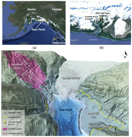
Figure 1.
The landslide source area. (a) The location of Taan Fiord, southern Alaska (using Google Earth Pro) (b) Location of the landslide source area in relation to Taan Fiord (using Google Earth Pro). (c) The landslide source and corresponding impact area (modified from Franco et al. [47]).
On 17 October 2015, after a period of heavy rainfall, a massive landslide occurred at the terminus of Tyndall Glacier and induced a tsunami with a runup of up to 193 m [2], which was the fourth-highest tsunami ever recorded in the world [46]. The landslide released approximately 50 Mm [47] of rock into the Taan Fiord. The length and width of this landslide are approximately 1630 m and 915 m, respectively. The slide area is 1.234 km. The maximum thickness of the landslide body is 93 m (Figure 1), which means that the maximum depth of the sliding surface is around 100 m.
No one directly observed this landslide event. Although field surveys have been conducted and related research works have been performed [1,2,3,35,36,47,48,49], the triggering mechanism of this landslide is still not elucidated. Seismic waves from an earthquake about 500 km away arrived shortly before this landslide, and a few seconds of mild shaking occurred [2], which could also be a possible trigger of this event. The precipitation in this area before this event (a month of above-average rain) was also higher than usual [2], which was also not beneficial to the stability of this slope. Glacier retreat and thinning due to climate change weakening the support of the toe of the slope was also observed in this area.
Previous studies related to this landslide event were conducted in 2015, including the geological and geomorphological conditions of this area. For example, Meigs et al. [34,50] investigated the ultra-landscape response and sediment yield following glacier retreat in this area, and described the scarps within the slope. After this landslide event, more research was conducted on landslide and landslide-generated tsunami phenomena in this area. For example, Higman et al. [2] conducted the field investigations and their field observations provided a benchmark for the landslide and tsunami hazards modelling. Haeussler et al. [35] focused on the submarine observations of bathymetry, submarine seismic profiling and surface change, and calculated the total volume of this landslide, including the volume that entered the fiord. Dufresne et al. [3] described the landslide mass and the landslide deposit using the debris on land, supra-glacial debris and submarine deposition. George et al. [1] presented a new methodology with the D-Claw model to compute the tsunami generation by the subaerial landslide. Gualtieri et al. [48] carried out a broadband analysis of the seismic signals by this landslide event, deduced the mass, trajectory and characteristics of the landslide dynamics, and also estimated the landslide volume to be about 55 million cubic meters. Williams et al. [49] analyzed the geomorphic and sediment accumulation history of Taan Fiord for the Tyndall Glacier retreat for over 50 years, and carried out a comparison of glacial and paraglacial denudation responses to rapid glacier retreat. Bloom et al. [36] investigated the characteristic modifications of the fan deltas in Taan Fiord, which were associated with the tsunami. Franco et al. [47] simulated a tsunami event in Taan Fiord with Flow-3D to verify the validity of the applied numerical models in reproducing the wave dynamics. Although many scientists have analyzed and studied the tsunami generated after the landslide event and its effects, only rudimentary related geotechnical investigations are performed on the 2015 Taan Fiord landslide (called the Taan landslide later in this paper).
2. Data and Materials
2.1. Geological and Structural Setting
The slope is located on the St. Elias Mountains, which is the product of the collisional history of the Yakutat terrane and the North American continent, the world’s highest coastal mountain range [3,51]. The topographical relief of this area has changed due to the collision between microplates and the influence of the external natural environment, e.g., the impact of the 2015 landslide event. The data collected with various remote-sensing methods were used to derive several Digital Elevation Models (DEM), from which essential information such as the topography and altitudes of different places in this area were collected [47]. Table 1 summarizes the different remote-sensing campaigns and the derived DEMs, which are used for analysis from 2000 to 2016. The DEM data for the Taan Fiord area are provided by the Elevation Portal of Alaska—Discrete Global Grid System (DGGS) and Haeussler et al. [35] for the years 2000–2014 and 2016, respectively. For the Taan Fiord in October 2015, just before the landslide occurred, a reconstructed, pre-collapse model based on the Interferometric synthetic aperture radar (InSAR) DEM of 2012 by George et al. [1] was presented. Since 2017, a new dataset (Arctic DEM AK V.2-2014, see Table 1) is available, and was used to update the landslide volume estimation just before the final collapse. The topographic surface after this catastrophic landslide was created by Haeussler et al. [35].

Table 1.
Summary of the Digital Elevation Models (DEM) and related information from different sources (modified from Franco et al. [47]).
In comparison to the DEMs of 2012 and 2016, the Arctic DEM-2014 shows significant elevation and horizontal offsets [47,52]. To obviate this disagreement, a re-projection and a co-registration were applied for the Artic DEM-2014. The re-projection process is conducted by the “Coordinate transformation (Grid)”, a tool in SAGA GIS [53] (Tool Libraries, Projection, Proj.4). The result provides a better re-adaption of the chosen digital model on the referred EPSG (in this case, 32607, WGS84/UTM zone 7N) and the related DEM of 2016 (from Haeussler et al. [35]). Initially, a manual co-registration with a mean offset of 25 m in a vertical direction was used. The result gave a good correspondence between the Arctic DEM-2014 and the one of 2016, with an accuracy of ±10 m in the vertical direction [47]. This accuracy was shown to be sufficient to identify very large mass movements.
However, some horizontal discrepancies were still present after manual correction. Thus, a co-registration process was performed for the DEMs of 2014 and 2016 to the DEM of 2012 with the method by Nuth and Kääb [54]. For this “demcoreg”, which is a collection of python and shell scripts, was utilized [55]. For the co-registration process, some stable sections (e.g., sections that are non-glaciated, or without mass movements or rockfalls) were selected in this area. Those areas have been highlighted in purple in Figure 2a. For the results before and after the co-registration process, Figure 2b–d show the shifts in the form of histograms for the difference in elevation values (m) from the DEM of 2014 to the one of 2012, the DEM of 2016 to the one of 2014 and the DEM of 2016 to the one of 2012, respectively. The result gives a better correspondence of the corrected digital model with an accuracy of ±5 m. The corresponding statistics resulting from the co-registration process are shown in Table 2. It can be seen that the Root Mean Square Difference (RMSD) between the DEMs of 2014 and 2012 and between the DEMs of 2016 and 2014 reduced to 2.03 and 1.85, respectively, after the co-registration process. The statistics seem to be reasonable when considering high geomorphological dynamics and the high variability in the snowpack in this area over the year.
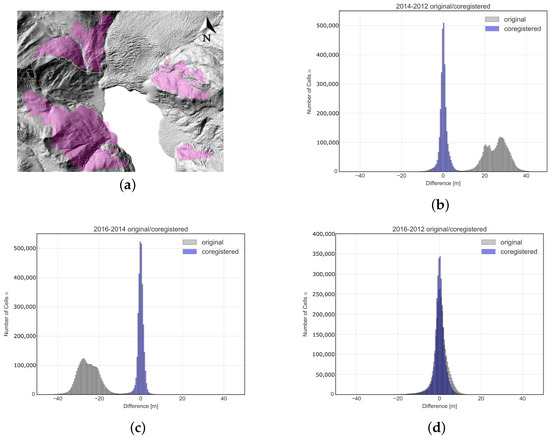
Figure 2.
The selected stable sections in this area and corresponding results for the co-registration process. (a) The selected stable sections (in purple) in this area used for the co-registration process. (b) The histogram showing the shift in the difference in elevation values (m) for the Digital Elevation Model (DEM) from 2014 to the one of 2012 after the co-registration process. (c) The histogram for the DEM from 2016 to the one of 2014. (d) The histogram for the DEM from 2016 to the one of 2012.
Table 2.
The statistics of difference indicators resulting from the co-registration process (Unit: m).
The geomorphological analysis is given using the open source software QGIS [56] and SAGA GIS. To be consistent with the analysis, some digital elevation models were downsampled to a resolution of 5 m with the method of bicubic spline interpolation that is available in SAGA GIS. Utilizing the raster calculator method implemented in QGIS, the difference in elevation for the landslide area from 2000 to 2016 can be obtained and is shown in Figure 3. In this period, especially after this catastrophic landslide, the elevation at different slope locations changed a lot. For the vertical displacement, a maximum negative value (mass loss) of 180 m and a positive value (material deposition) of 60 m are observed in this area.
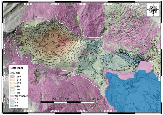
Figure 3.
DEM of difference (DOD) [57] for the landslide area from 2000 to 2016. The white dotted line represents the margin of the landslide area. The purple colour corresponds to the lack of identified changes in elevation for locations of the slope or the glacier (Figure exported from QGIS).
Before the year 2000, some facing scarps on the upper part of this slope were already present, as illustrated in the work of Meigs et al. [34]. Based on the aerial photographs and mapping [34], a mountain-scale landslide failure of the fiord wall was detected between 1983 and 1996. This documented landslide covered an area of approximately 0.4 km, and a head scarp of about 200 meters appeared with a dip of around 60°. The resulting head scarp cross-cut the bedrock structure and struck subparallel to the fiord wall [34].
To analyse possible triggers of the 2015 Taan landslide, some studies refer to the glacial retreat [3,36,49], as well as to a large amount of precipitation before the occurrence of this landslide or frequent earthquakes in this area [2]. George et al. [1] also put forward that the mobilization of 2015 Taan landslide cannot be directly attributed to the glacial retreat, as the old slump was suggested to be a result of the instability caused by postglacial deglaciation and the consequent increase in valley wall height [34], while the height of the valley wall in this area did not significantly increase from 1996 to 2015.
Regarding the pre-evolution and formation process of the 2015 Taan landslide, Franco et al. [47] gave a four-stage interpretation of the landslide dynamics: (1) Before the year 2000, slope instability may be induced due to the fast ice loss and glacier retreat, which leads to the formation of internal antithetic discontinuities or local normal faults with a dip ranging between 60° and 80° against the slope; (2) Before the year 2012, the slope may have undergone some minor rotational displacements, such as a rigid body, rotating counter clockwise by about 20° to 30°; (3) After the year 2012, the orientation of these internal discontinuities gradually changed and shifted to a sub-vertical dip due to the rotation of the sliding mass. This led to a sudden significant vertical displacement during the period from 2012 to 2014; (4) In the years prior to the 2015 landslide event, the glacial retreat may lead to the final collapse due to its weakened buttressing effect. A schematic diagram that can be used to interpret the landslide dynamics prior to slope failure is shown in Figure 4.
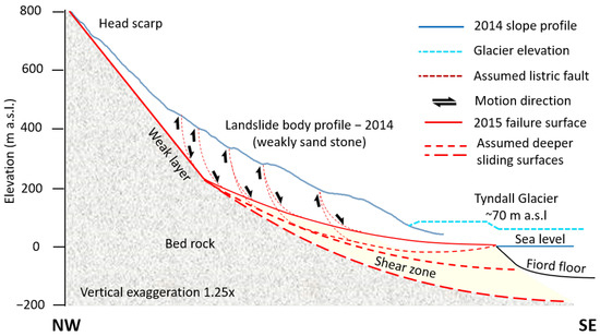
Figure 4.
Interpretation of the landslide dynamics and the possible evolution of the sliding surface before the landslide (modified from Franco et al. [47]).
It is not known whether the rotation of the sliding mass was caused by deformation along the newly formed, internal discontinuities prior to 2012. The actual triggers that led to the 2015 landslide event are also unknown, as well as the causes of the newly formed discontinuities within the slope. Therefore, a detailed investigation of possible failure processes and triggers is presented in the study.
In the area around the location of the Taan landslide, there is a Chaix Hills Thrust fault along the east–west orientation. There are several known stratigraphic units for this fault, e.g., the Kulthieth Formation and the Yakataga Formation [3]. For the stratigraphy of Taan landslide site, the Kulthieth Formation dominates. This consists of interlayered sandstone, coals, mudstones, and conglomerates [58]. Due to the ongoing collision of the Yakutat microplate with North America, the surface compositions of the this slope are weakly lithified sedimentary rocks [59].
The geotechnical parameters (e.g., soil cohesion or friction angle) are unavailable for the slope, which provides a huge challenge for geotechnical analysis. Since the geological compositions of this area are dominated by sand- and mudstone, the friction angle should be correspondingly large, and their cohesion is closely related to the ratio of each component and the degree of weathering. As the surface of this slope is severely affected by weathering, its strength parameters should be close to those of weathered sandstone or mudstone. Based on their similar geological composition, the strength parameters of this slope could be estimated accordingly, by referring to the range of values taken from the other literature, i.e., the cohesive strength lies between a few tens and a few hundreds of kPa, and the friction angle is usually between 30° and 50° (and between 40° and 50° in many cases) [60,61,62,63,64,65,66,67,68,69,70,71,72,73,74]. The literature review of strength parameters with a similar geological composition can be seen in Table 3.
Table 3.
Literature review of strength parameters (Mohr–Coulomb criterion) with similar geological composition (sorted by year of publication).
2.2. The Cross Sections
For this study, the elevation changes in this slope and the adjacent glacier are investigated by selecting representative cross-sections in the area (Figure 5). The slope profiles of different years in Figure 5b are at the location of the cross-section S-S’ in Figure 5a. The profile data from 2000 to 2014 in Figure 5b are also provided by the Elevation Portal of Alaska—DGGS. The data for the years 2015, when the landslide occurred, and 2016, after the slope collapse, are based on the work of George et al. [1] and Haeussler et al. [35], respectively.
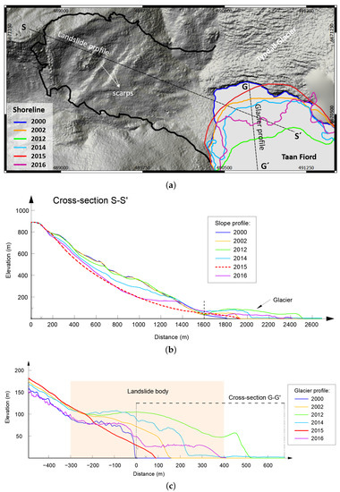
Figure 5.
Surface conditions and elevation changes for the slope and glaciers at different landslide site positions since 2000 (all locations or profiles for the year 2015 are reconstructed on the basis of the work of George et al. [1]). (a) The shoreline (or the location of the glacier edge) from 2000 to 2016. The bold black solid line represents the landslide area. The black dash line S-S’ represents the location of the cross-section for slope profiles in (b), the black dash line G-G’ represents the location of the cross-section for glacier profiles in (c). (b) Slope profiles along the cross-section S-S’ in (a) from 2000 to 2016. The profiles from 2000 to 2014 are from the data of DGGS. The profile of 2015 refers to the recreated sliding surface from the work of George et al [1]. The profile of 2016 is from the work of Haeussler et al. [35]. (c) The glacier elevation variation (vertical exaggeration 2×) at the cross-section G-G’ in (a). Information is taken from Franco et al. [47].
Since the slip surfaces of rotational landslides are commonly assumed with log-spiral shapes [1], George et al. made such an approximation of the landslide basal slip surface by fitting logarithmic spirals along three longitudinal transects (one approximately at the cross-section S-S’ and the other two at both sides of this cross-section), which are orthogonal to the scarps within the landslide. The logarithmic spirals are constrained by the inferred scarp and toe inclinations. The slope profiles along this cross-section represent the change in the elevation of the slope surface from 2000 to 2016, and also show the change in glacier thickness at the toe of this slope during this period. Two main changes can be seen in the elevation of the slope surface: one could be due to internal rotation in the period from 2012 to 2014 and one due to the plunge in elevation caused by the landslide event in 2015. For the change in glacier thickness at the foot of the slope, the glacier gradually retreated and continuously decreased in thickness from 2012 to 2015, which gradually lowered the buttressing effect on the slope.
Since there is a relatively large angle of about 63° between the central axis of the landslide area and the central axis of the Tyndall Glacier terminus area, the cross-section S-S’ is not a complete representation of the glacier thickness. Figure 5c reflects the change in the thickness of Tyndall Glacier at the terminus, and Figure 5a shows the corresponding change in shoreline position from 2000 to 2016. The glacier position at the terminus of Tyndall Glacier alternated between advancing and retreating between 2000 and 2012, with an overall advancing trend. Between 2012 and 2015, the glacier position receded sharply, which is also visible in the profile plots at the cross-section S-S’ in Figure 5b. In 2016, after this slope collapse, the glacier position advanced again.
3. Methods
The purpose of this case study is to investigate and verify the possible triggers and processes of this landslide using two-dimensional limit equilibrium analysis. To facilitate a comparison of the results, all calculation results in this paper were obtained with the Morgenstern–Price method.
The computational model is based on the slope profile of 2014 at the cross-section S-S’, as shown in Figure 5. Since the geotechnical parameters and internal strength distribution of this slope are not available, a homogeneous material is assumed for the slope body (weak lithified stone). In the calculation model, as shown in Figure 6, the horizontal starting point of the cross-section S-S’ in this study area is also the zero point of x-coordinate (distance is zero in Figure 5b), and the elevations are the y-axis coordinates. Since the altitude of the mountain does not vary much within a few hundred meters uphill from the starting point of the known cross-section, away from the Taan Fiord, which is at a height of approximately 900 m, the model is extended by 100 m along the horizontal and vertical directions, respectively, to reduce the artificial constraints.
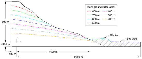
Figure 6.
Different groundwater tables in the calculation based on the 2014 slope profile.
The height of this slope is about 890 m, the horizontal length is about 1700 m, and the average slope is slightly less than 30°, with a steeper upper part and a gentler lower part of about 35° and 20°, respectively.
The groundwater level in this slope is also unknown, which makes it difficult to analyze the effect of precipitation on slope stability. To account for the influence of groundwater on the results, different groundwater levels were adopted for seepage and no-seepage conditions. In Slide (a Rocscience software), the resulting groundwater table is obtained based on the steady-state groundwater calculation. Setting the height of the groundwater table at the left boundary (uphill-side, at the position with a horizontal coordinate of −100 m) of this model as the initial groundwater table, as shown in Figure 6, different steady-state tables were adopted in the calculation, marked by dashed lines of different colors, ranging from 800 m to 200 m. The range of values for the groundwater table in calculations is listed in Table 4. We emphasize that this is a wide range of possible groundwater tables, and which one leads to realistic results will be revealed later (see Section 4).
Table 4.
The range of values for the groundwater table in calculation.
In the calculation model, the parameter values of geotechnical materials are based on the literature review of cases with a similar geological composition. The density values of sandstones are usually between 2150 and 2650 kg/m [76]. The values of 2350 kg/m [2] and and 2700 kg/m [48,77] are also adopted in the estimation of landslide mass. Based on rocks with a similar composition, age and burial history from the the Susitna and Cook Inlet basins, Alaska [78,79], the density of the landslide material is estimated as 2350 kg/m. Combining the reported density values, we chose 2450 kg/m. Thus, the unit weight for the geotechnical materials of the slope is taken as 24 kN/m. The values of the strength parameters for the slope body will be discussed in combination with the analysis. The unit weight for the glacier is taken as 9 kN/m, since it is composed entirely of ice. Based on the typical values for the Mohr–Coulomb parameters of ice [80,81], 4.5 MPa and 6° are adopted for the strength parameters of the glacier, i.e., the cohesion and the internal friction angle, respectively.
4. Results and Discussion
4.1. Preliminary Slope Stability Analysis
First, some preliminary calculations were performed to investigate the effect of precipitation on the position of possible sliding surfaces. The Mohr–Coulomb parameters were adopted for the landslide body in this section. Here, the combined, extreme values of the cohesion and friction angle of the involved materials were assumed to test their influence on the results. The cohesion is taken as 20 kPa or 100 kPa, while the friction angle is taken as 30° or 45° according to most of the strength parameters, which are defined by other authors for the same materials (Table 3). Therefore, there are four parameter combinations for the sliding mass (Table 5). The four sets of parameters are denoted as p1, p2, p3 and p4. The results are shown in Figure 7, and the FoS values calculated for different groundwater levels are listed in Table 6.
Table 5.
The four sets of shear strength parameters assumed for the sliding mass in the preliminary slope stability analyses.
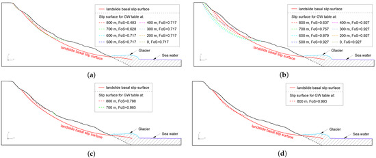
Figure 7.
Sliding surfaces for groundwater table at different levels. (a) The results for the parameter set of p1. (b) The results for the parameter set of p2.(c) The results for the parameter set of p3. (d) The results for the parameter set of p4.
Table 6.
The safety factors under different initial groundwater table conditions for the four parameter sets (p1, p2, p3 and p4) as a preliminary attempt.
In Figure 7, the red line represents the position of the assumed slip surface in the 2015 Taan landslide. The four subfigures show that the sliding surfaces appear only in the upper part of this slope, regardless of the high or low groundwater levels, when only the effect of precipitation on the slope stability is considered. This is not the most probable actual location of the sliding surface in the 2015 Taan landslide. This is also true when performing the calculation with a predefined discontinuity in only the upper part according to Figure 4. Moreover, since the calculated sliding surface remains well above the toe of this slope, the glacial retreat does not have a strong influence on the location of the failure surface.
The outcomes of the preliminary 2D limit equilibrium calculations revealed that a sliding surface close to the assumed shear zone in 2015 Taan landslide could not appear if only the influences of glacial retreat and different groundwater levels are considered. This suggests that the glacier retreat in the decades before 2015 may have had an impact on the stability of this slope during the formation of the internal discontinuities, but was perhaps not the direct, dominant factor in its generation throughout the whole slope body.
These seemingly unsuccessful preliminary attempts led us to think more deeply about the triggers of this landslide event and the evolution of highly likely discontinuities, which have a critical impact on slope stability. Based on preliminary calculations, various influencing factors and possible discontinuities are taken into account in the simulation and analysis of slope failure in the following sections.
4.2. The Formation of a Weak Basal Layer
As the slope is in the earthquake-prone zone, the influence of earthquakes on the stability of this slope cannot be ignored. Large-magnitude historical earthquakes led to active faults in this area, e.g., earthquakes with M8.2 in 1899 and seven earthquakes >M6 since 1958 [3]. Peak ground motions generated by nearby earthquakes are important in earthquake safety analysis for slopes, especially the peak ground acceleration. In general, the horizontal acceleration generated by earthquakes can have an impact on the stability of the slope, and even on the shape and location of the sliding surface when a landslide occurs, while the vertical acceleration is usually neglected [82] especially in the conventional pseudo-static slope stability assessment. From the information available on the United States Geological Survey (USGS) website, combined with the empirical formulae [83,84] for the horizontal peak ground acceleration (PGA) generated by earthquakes, several earthquakes near the landslide site were found to generate horizontal accelerations of 0.3 g or even larger at this region before the 2015 Taan landslide.
One new hypothesis for a possible interpretation of the historical formation process of the internal weak layers in the slope and the process of landslide occurrence is as follows. On the whole, the landslide formation could be broadly separated into two stages: (1) With earthquakes and precipitation as the possible main influencing factors, multiple destabilizations of this slope occurred and, accordingly, the sliding mass moved several times; however, there was no overall slope collapse. These motions caused shear deformations within the slope, which were localized in a relatively small shear band. The landslide body initially consisted of weathered rock, and the shear zone was most probably a granular material, which is produced by crushing the original rock mass. This crushing led to the disintegration of the material, resulting in a lower shear strength. Obviously, this decrease in shear strength was not strong enough to yield a final collapse; however, a zone of lower-strength material remained, which we call a weak layer. (2) Despite the presence of this weak layer, the slope did not fail (FoS > 1) due to the buttressing effect provided by the glacier at the toe of the slope. Before the 2015 Taan landslide, the glacier substantially retreated, causing a loss of support at the slope toe and triggering this large-scale landslide. To account for the assumed two stages of landslide formation, the below analyses follow these two stages: the formation of a weak layer, and the final slope collapse.
In the first stage of calculation, groundwater level and seismic intensity are investigated as influencing factors of the calculation results. As illustrated in above sections, different groundwater levels are adopted (Table 4). Similarly, different horizontal acceleration values for seismic loading (0.0 g, 0.1 g, 0.2 g, 0.3 g, 0.4 g and 0.5 g) were adopted in the calculations (Table 7).
Table 7.
The range of values for the horizontal seismic load coefficient in calculation.
4.2.1. The Influence of Groundwater Level
The two main investigated factors are the height of groundwater table and the seismic load. Their effects are correlated, and we begin with the influence of the groundwater table height for two exemplary seismic loads. The mechanical parameters of the basal weak layer and overlying sliding mass (e.g., unit weight, strength parameters) are listed in Table 8 as the input for the material properties in the caluclation model. As illustrated in the above section, the cohesion and friction angle of weathered rock with a mixture of sandstone and mudstone are usually between a few tens and hundreds of kPa, and 30° to 50°, respectively. As an example, the Mohr–Coulomb parameters for Set 1 were as follows: cohesion and internal friction angle were taken as 100 kPa and 45°, respectively. Since no significant differences were found in the results of the computations with parameter Set 1 and 2, only the results of parameter Set 1 are presented.
Table 8.
The material properties assumed in the limit equilibrium method (LEM) analyses.
Since the location of the calculated sliding surface significantly differs from that assumed for the 2015 landslide when seismic loading is not considered, the results are compared for different groundwater levels under the horizontal seismic acceleration conditions of 0.3 g and 0.2 g, as shown in Figure 8 and Figure 9. The corresponding FoS values are listed in Table 9. Other seismic accelerations are investigated in the following subsection.
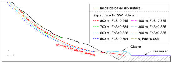
Figure 8.
Sliding surfaces for different levels of the groundwater table under the seismic acceleration of 0.3 g (the slip surface corresponding to the GW table with black underlines in the legend is closest to the observed slip surface).
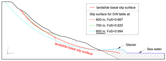
Figure 9.
Sliding surfaces for different levels of the groundwater table under the seismic acceleration of 0.2 g (the slip surface corresponding to the GW table with black underlines in the legend is closest to the observed slip surface).
Table 9.
The safety factors of the slope under different initial groundwater table conditions for the seismic loading of 0.2 g or 0.3 g.
For a seismic acceleration of 0.3 g, the most likely sliding surface occurs in the upper part of this slope when the groundwater table is very high (e.g., initial groundwater table is 700 m or 800 m) or very low (e.g., initial groundwater table less than or equal to 400 m). For cases with low groundwater levels (less than or equal to 400 m or without considering the groundwater), sliding surfaces appear at the same location, as they are not affected by the groundwater. Moreover, the sliding surfaces resulting from the very low groundwater table conditions are located slightly higher than those computed with very high groundwater levels. For an initial groundwater table at a moderate level, e.g., 600 m or 500 m, the sliding surface cuts through the entire slope from the top to the bottom, and is close to the position of the assumed Taan landslide slip surface (red solid line). It is also noted that the sliding surface for an initial groundwater table of 600 m is more close to the assumed slip surface than that of 500 m.
For the seismic acceleration of 0.2 g, the sliding surface locations resulting from high and low groundwater tables have similar characteristics to those of the 0.3 g case. However, for the medium groundwater table, the sliding surface location produced by the initial groundwater table of 600 m is slightly deeper than that of the 0.3 g condition, which is closer to the assumed slip surface. For an initial groundwater table less than or equal to 500 m, the slope did not fail (FoS > 1). The calculation results for the seismic acceleration condition of 0.3 g are, therefore, more realistic than that of 0.2 g.
Futher results of a large number of calculations, conducted by adopting different geotechnical parameters (cohesion: 50 kPa to 500 kPa, friction angle: 30° to 50°), show that the sliding zone under moderate groundwater level and seismic loading conditions is relatively close to the observed Taan landslide slip surface.
4.2.2. The Influence of Horizontal Seismic Acceleration
To investigate the influence of different seismic accelerations on the calculation results, two sets of geotechnical parameters and an initial groundwater table at 600 m are selected. Cohesions and friction angles in these two sets of Mohr-Coulomb parameters (Set 1 and Set 2 in Table 8) are 100 kPa and 45°, and 120 kPa and 50°, respectively. The resulting slip surfaces for these two sets under different seismic load conditions are shown in Figure 10 and Figure 11. The corresponding FoS values for the two sets are listed in Table 10.
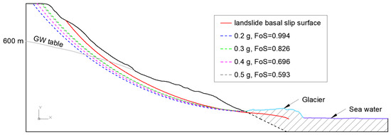
Figure 10.
Sliding surfaces obtained under different seismic acceleration conditions for Set 1.
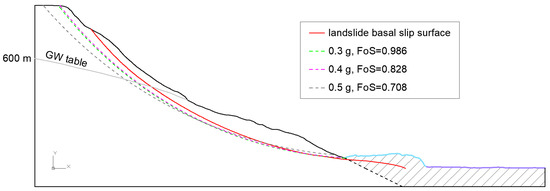
Figure 11.
Sliding surfaces obtained under different seismic acceleration conditions for Set 2.
Table 10.
The safety factors under different seismic load conditions for both parameter sets.
Since the upper part of this slope is relatively steep, the most likely sliding surface is located in the upper part of this slope when no earthquake is considered or when the earthquake acceleration is relatively small, and the FoS values are larger than 1 for these two parameter sets. When the seismic acceleration is no less than 0.2 g, the most likely sliding surface is located from the top to the toe of the slope. When the seismic acceleration is relatively large (≥0.3 g), the sliding surface is more close to the assumed Taan landslide slip surface than that with small seismic loading (≤0.2 g), which is also reflected in the previous analysis of the groundwater level effects.
By comparing the results for different parameter values, the potential sliding surface calculated under the seismic condition was found to be very close to the actual sliding surface location assumed for the Taan landslide when the Mohr–Coulomb parameters were within a certain range. For example, a well-fitted result could be obtained when the friction angle was around 45° (±5°), the cohesion was around 100 kPa (±20 kPa), the initial groundwater table was around 0.65 (±0.05) times the slope height and the horizontal seismic acceleration was at least 0.2 g (better for ≥0.3 g).
Since the obtained safety factor is only slightly less than 1 (usually larger than 0.8), this sliding only produces a relatively small displacement during the earthquake. The block mass above the shear zone slid for a certain distance, and the slope returned to a stable state after the earthquake, fitting the main assumption of any displacement estimation based on the Newmark method [85]. One can assume that several such movements occurred within a small distance in the decades before the 2015 Taan landslide. Due to the block mass movement above a localized shear zone, a weak layer developed within the slope, called a fault.
4.3. The Final Slope Collapse
In the 2D LEM analyses, the weak shear zone at the base of the landslide, formed during the first slope instability stage, was considered a discrete sliding surface. The sliding surface was modelled as a pre-defined discontinuity with the shear strength parameters of the weak layer. To calculate the second stage, the glacial retreat at the toe of this slope was focused on as a trigger of the Taan landslide. Since there was only one mild shaking, from a small earthquake far from this site, shortly before the Taan landslide in 2015, the seismic loading was not considered in the calculations in this phase. The two sets of Mohr–Coulomb parameters (Set 1 and Set 2; see Table 8) are still used for the analysis with two scenarios—with and without glaciers at the toe of this slope—as shown in Figure 12.
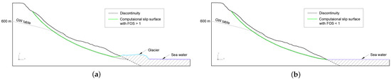
Figure 12.
The locations of the weak layer and resulting computational slip surface with the initial groundwater table at 600 m. (a), with the glacier at the toe based on the 2014 slope profile. (b) without the glacier.
Based on the values taken in the previous subsection, the height of the groundwater table at the left boundary was taken as 600 m. The parameters of the weak layer were assumed to be different from the overlying sliding mass due to the shearing process that occurred in recent decades. To set the Mohr–Coulomb parameters at the weak layer position, the cohesion is usually small and the friction angle is reduced to some extent. For example, the strength of the material in the shear zones of deep seated landslides, measured by Strauhal et al. [86], is rather low.
Four sets of Mohr–Coulomb parameters (a1 and a2, b1 and b2) were chosen as the strength parameters of the weak layer, summarized in Table 8. These values represent the weakened material in the evolved shear zone. The results of the safety factors for these four cases are listed in Table 11.
Table 11.
Safety factors for the 4 cases (a1 and a2 for the weak layer in the case of Set 1, b1 and b2 for the weak layer in the case of Set 2, see Table 8), with and without the glacier at the toe.
The results clearly show that the safety factor obtained under the condition with the glacier at the toe was greater than 1, while the result under the condition without glacier was less than 1. This indicates that the glacier at the toe had a buttressing effect on the slope, and, during the period from 2014 to 2015, before the landslide occurred, the glacier at the toe melted and substantially retreated, which caused the buttressing effect at the toe to weaken, and the safety factor of this slope gradually decreased. The influence of the glacier, together with a combination of factors such as a larger than usual amount of rainfall in September and October in 2015, before the landslide, and a mild shaking due to the small earthquake in the distance, all contributed to the occurrence of this large landslide event.
5. Conclusions
In this work, a geotechnical study on the 2015 Taan Fiord landslide is provided, where stability analyses were carried out by employing 2D–LEM. Diverse possible external triggers for the landslide were investigated. The available DEMs were co-registered and used to better understand the morphological evolution of this coastal landslide. Representative cross-sections (of both slope and glacier body) were derived from DEMs for further numerical investigation. The main conclusions are as follows:
(1) In the first stage of landslide formation, earthquakes are critical to the formation of a weak basal layer. The LEM analyses carried out on the 2015 Taan landslide qualitatively demonstrated that rainfall and seismic ground motions may have initiated the slope instability process.
(2) In the second stage of landslide formation, the final slope collapse resulted from glacial retreat at the toe of the slope. The weak basal layer formed in the first stage acted as the final sliding zone.
Remote-sensing data can be employed to constrain slope stability analyses to reconstruct the morphology of the slope when direct topographical data are lacking. This is especially true when multi-temporal aerial radar data are also available, as this paper demonstrates. In this interdisciplinary approach, the limit equilibrium method applied to sections of the DEMs is well-suited to identifying weak layers and possible formation processes. In this case, the weak layer likely formed through previous earthquake activities. The final triggering factor was most probably a combination of glacier retreat and precipitation.
Although the geotechnical parameters of the slope are unavailable in this study, plausible calculation results are obtained and the location of the calculated weak layer is close to the actual observed sliding surface location. This is achieved by parameter studies, in combination with reasonable reference values of similar conditions in other papers. This can also illustrate the applicability of the 2D limit equilibrium analysis in the analysis of large-scale landslides under complex conditions.
Finally, this study effectively confirms the importance of an interdisciplinary approach that combines aerial radar data and traditional slope stability analyses. The implications of climate change for landslide hazard assessment and the interaction of physical processes in a multi-hazard context cannot be ignored.
Author Contributions
Conceptualization, X.D., B.S.-M. and W.F.; methodology, X.D., B.S.-M. and W.F.; software, X.D.; validation, X.D.; formal analysis, X.D., B.S.-M. and W.F.; investigation, X.D.; resources, B.S.-M., A.F. and B.G.; data curation, X.D.; writing—original draft preparation, X.D. with partial contribution of B.S.-M. and W.F.; writing—review and editing, B.S.-M., W.F., A.F. and B.G.; visualization, X.D.; supervision, B.S.-M. and W.F.; project administration, B.S.-M. and W.F.; funding acquisition, B.S.-M. and W.F. All authors have read and agreed to the published version of the manuscript.
Funding
This research is funded by the University of Innsbruck in support of the doctoral program “Natural Hazards in Mountain Regions”. Open access funding is provided by the Vice Rectorate for Research of the University of Innsbruck.
Institutional Review Board Statement
Not applicable.
Informed Consent Statement
Not applicable.
Data Availability Statement
The data that support the findings of this study are available from the corresponding author upon reasonable request.
Acknowledgments
The first author would like to acknowledge Bretwood Higman (Ground Truth Trekking, Seldovia, AK, USA) for answering the question via email reply in this study. A great thank is further owned to Andreas Huber (the University of Innsbruck, Unit of Hydraulic Engineering) for the support to efficient DEMs co-registration and the patient and detailed explanation. The authors also gratefully acknowledge the support of Johannes Branke for the help in revising the manuscript. We thank the two anonymous referees for their constructive comments, which helped to improve the presentation of this paper.
Conflicts of Interest
The authors declare no conflict of interest.
References
- George, D.; Iverson, R.; Cannon, C. New methodology for computing tsunami generation by subaerial landslides: Application to the 2015 Tyndall Glacier landslide, Alaska. Geophys. Res. Lett. 2017, 44, 7276–7284. [Google Scholar] [CrossRef]
- Higman, B.; Shugar, D.H.; Stark, C.P.; Ekström, G.; Koppes, M.N.; Lynett, P.; Dufresne, A.; Haeussler, P.J.; Geertsema, M.; Gulick, S.; et al. The 2015 landslide and tsunami in Taan Fiord, Alaska. Sci. Rep. 2018, 8, 1–12. [Google Scholar] [CrossRef] [PubMed]
- Dufresne, A.; Geertsema, M.; Shugar, D.; Koppes, M.; Higman, B.; Haeussler, P.; Stark, C.; Venditti, J.; Bonno, D.; Larsen, C.; et al. Sedimentology and geomorphology of a large tsunamigenic landslide, Taan Fiord, Alaska. Sediment. Geol. 2018, 364, 302–318. [Google Scholar] [CrossRef]
- Cruden, D.M.; Varnes, D.J. Landslide Types and Processes. Spec. Rep.-Natl. Res. Counc. Transp. Res. Board 1996, 247, 36–75. [Google Scholar]
- Dai, F.; Lee, C.; Ngai, Y. Landslide risk assessment and management: An overview. Eng. Geol. 2002, 64, 65–87. [Google Scholar] [CrossRef]
- Haque, U.; Blum, P.; Da Silva, P.F.; Andersen, P.; Pilz, J.; Chalov, S.R.; Malet, J.P.; Auflič, M.J.; Andres, N.; Poyiadji, E.; et al. Fatal landslides in Europe. Landslides 2016, 13, 1545–1554. [Google Scholar] [CrossRef]
- McColl, S.T. Landslide causes and triggers. In Landslide Hazards, Risks and Disasters; Elsevier: Amsterdam, The Netherlands, 2015; pp. 17–42. [Google Scholar] [CrossRef]
- Marui, H.; Nadim, F. Landslides and multi-hazards. In Landslides–Disaster Risk Reduction; Springer: Berlin/Heidelberg, Germany, 2009; pp. 435–450. [Google Scholar] [CrossRef]
- Keefer, D.K. Landslides caused by earthquakes. Geol. Soc. Am. Bull. 1984, 95, 406–421. [Google Scholar] [CrossRef]
- Sassa, K.; Fukuoka, H.; Scarascia-Mugnozza, G.; Evans, S. Earthquake-induced-landslides: Distribution, motion and mechanisms. Soils Found. 1996, 36, 53–64. [Google Scholar] [CrossRef]
- Rodríguez, C.; Bommer, J.; Chandler, R. Earthquake-induced landslides: 1980–1997. Soil Dyn. Earthq. Eng. 1999, 18, 325–346. [Google Scholar] [CrossRef]
- Bommer, J.J.; Rodríguez, C.E. Earthquake-induced landslides in Central America. Eng. Geol. 2002, 63, 189–220. [Google Scholar] [CrossRef]
- Stead, D.; Eberhardt, E. Understanding the mechanics of large landslides. Ital. J. Eng. Geol. Environ. 2013, 6, 85–112. [Google Scholar] [CrossRef]
- Kos, A.; Amann, F.; Strozzi, T.; Delaloye, R.; Ruette, J.; Springman, S. Contemporary glacier retreat triggers a rapid landslide response, Great Aletsch Glacier, Switzerland. Geophys. Res. Lett. 2016, 43. [Google Scholar] [CrossRef]
- Hutter, K. Theoretical Glaciology; Springer: Dordrecht, The Netherlands, 1983. [Google Scholar] [CrossRef]
- McColl, S.; Davies, T.; McSaveney, M. Glacier retreat and rock-slope stability: Debunking debuttressing. In Geologically Active; Taylor and Francis: London, UK, 2010; pp. 467–474. [Google Scholar]
- Derbyshire, E.D. Geomorphology and Climate; Wiley Chichester: London, UK, 1976. [Google Scholar]
- Collins, B.D.; Znidarcic, D. Stability analyses of rainfall induced landslides. J. Geotech. Geoenviron. Eng. 2004, 130, 362–372. [Google Scholar] [CrossRef]
- Wu, L.; Huang, R.; Xu, Q.; Zhang, L.; Li, H. Analysis of physical testing of rainfall-induced soil slope failures. Environ. Earth Sci. 2015, 73, 8519–8531. [Google Scholar] [CrossRef]
- Zhu, D.; Lee, C.; Jiang, H. Generalised framework of limit equilibrium methods for slope stability analysis. Geotechnique 2003, 53, 377–395. [Google Scholar] [CrossRef]
- Brideau, M.A.; Stead, D.; Couture, R. Structural and engineering geology of the east gate landslide, Purcell Mountains, British Columbia, Canada. Eng. Geol. 2006, 84, 183–206. [Google Scholar] [CrossRef]
- Bolla, A.; Paronuzzi, P. Numerical investigation of the pre-collapse behavior and internal damage of an unstable rock slope. Rock Mech. Rock Eng. 2019, 53, 2279–2300. [Google Scholar] [CrossRef]
- Sloan, S. Geotechnical stability analysis. Géotechnique 2013, 63, 531–571. [Google Scholar] [CrossRef]
- Zienkiewicz, O.C.; Humpheson, C.; Lewis, R. Associated and non-associated visco-plasticity and plasticity in soil mechanics. Geotechnique 1975, 25, 671–689. [Google Scholar] [CrossRef]
- Eberhardt, E.; Stead, D.; Coggan, J. Numerical analysis of initiation and progressive failure in natural rock slopes—The 1991 Randa rockslide. Int. J. Rock Mech. Min. Sci. 2004, 41, 69–87. [Google Scholar] [CrossRef]
- Tschuchnigg, F.; Schweiger, H.; Sloan, S.W. Slope stability analysis by means of finite element limit analysis and finite element strength reduction techniques. Part I: Numerical studies considering non-associated plasticity. Comput. Geotech. 2015, 70, 169–177. [Google Scholar] [CrossRef]
- Tschuchnigg, F.; Schweiger, H.; Sloan, S.W. Slope stability analysis by means of finite element limit analysis and finite element strength reduction techniques. Part II: Back analyses of a case history. Comput. Geotech. 2015, 70, 178–189. [Google Scholar] [CrossRef]
- Schneider-Muntau, B.; Medicus, G.; Fellin, W. Strength reduction method in Barodesy. Comput. Geotech. 2018, 95, 57–67. [Google Scholar] [CrossRef]
- Dawson, E.; Roth, W.; Drescher, A. Slope stability analysis by strength reduction. Geotechnique 1999, 49, 835–840. [Google Scholar] [CrossRef]
- Choi, S.K.; Park, J.Y.; Lee, D.H.; Lee, S.R.; Kim, Y.T.; Kwon, T.H. Assessment of barrier location effect on debris flow based on smoothed particle hydrodynamics (SPH) simulation on 3D terrains. Landslides 2021, 18, 217–234. [Google Scholar] [CrossRef]
- Conte, E.; Pugliese, L.; Troncone, A. Post-failure analysis of the Maierato landslide using the material point method. Eng. Geol. 2020, 277, 105788. [Google Scholar] [CrossRef]
- Xu, W.J.; Xu, Q.; Liu, G.Y.; Xu, H.Y. A novel parameter inversion method for an improved DEM simulation of a river damming process by a large-scale landslide. Eng. Geol. 2021, 293, 106282. [Google Scholar] [CrossRef]
- Puzrin, A.M.; Germanovich, L. The growth of shear bands in the catastrophic failure of soils. Proc. R. Soc. A: Math. Phys. Eng. Sci. 2005, 461, 1199–1228. [Google Scholar] [CrossRef]
- Meigs, A.; Sauber, J. Southern Alaska as an example of the long-term consequences of mountain building under the influence of glaciers. Quat. Sci. Rev. 2000, 19, 1543–1562. [Google Scholar] [CrossRef]
- Haeussler, P.; Gulick, S.; McCall, N.; Walton, M.; Reece, R.; Larsen, C.; Shugar, D.; Geertsema, M.; Venditti, J.; Labay, K. Submarine deposition of a subaerial landslide in Taan Fiord, Alaska. J. Geophys. Res. Earth Surf. 2018, 123, 2443–2463. [Google Scholar] [CrossRef]
- Bloom, C.K.; MacInnes, B.; Higman, B.; Shugar, D.H.; Venditti, J.G.; Richmond, B.; Bilderback, E.L. Catastrophic landscape modification from a massive landslide tsunami in Taan Fiord, Alaska. Geomorphology 2020, 353, 107029. [Google Scholar] [CrossRef]
- Sturzenegger, M.; Stead, D. The Palliser Rockslide, Canadian Rocky Mountains: Characterization and modeling of a stepped failure surface. Geomorphology 2012, 138, 145–161. [Google Scholar] [CrossRef]
- Francioni, M.; Salvini, R.; Stead, D.; Litrico, S. A case study integrating remote sensing and distinct element analysis to quarry slope stability assessment in the Monte Altissimo area, Italy. Eng. Geol. 2014, 183, 290–302. [Google Scholar] [CrossRef]
- Bonilla-Sierra, V.; Scholtes, L.; Donzé, F.; Elmouttie, M. Rock slope stability analysis using photogrammetric data and DFN–DEM modelling. Acta Geotech. 2015, 10, 497–511. [Google Scholar] [CrossRef]
- Cloutier, C.; Locat, J.; Couture, R.; Jaboyedoff, M. The anatomy of an active slide: The Gascons rockslide, Québec, Canada. Landslides 2016, 13, 241–258. [Google Scholar] [CrossRef]
- Zieher, T.; Schneider-Muntau, B.; Mergili, M. Are real-world shallow landslides reproducible by physically-based models? Four test cases in the Laternser valley, Vorarlberg (Austria). Landslides 2017, 14, 2009–2023. [Google Scholar] [CrossRef]
- Zieher, T.; Rutzinger, M.; Schneider-Muntau, B.; Perzl, F.; Leidinger, D.; Formayer, H.; Geitner, C. Sensitivity analysis and calibration of a dynamic physically based slope stability model. Nat. Hazards Earth Syst. Sci. 2017, 17, 971–992. [Google Scholar] [CrossRef]
- Tordesillas, A.; Kahagalage, S.; Campbell, L.; Bellett, P.; Intrieri, E.; Batterham, R. Spatiotemporal slope stability analytics for failure estimation (SSSAFE): Linking radar data to the fundamental dynamics of granular failure. Sci. Rep. 2021, 11, 1–18. [Google Scholar] [CrossRef]
- Bruhn, R.L.; Pavlis, T.L.; Plafker, G.; Serpa, L. Deformation during terrane accretion in the Saint Elias orogen, Alaska. Geol. Soc. Am. Bull. 2004, 116, 771–787. [Google Scholar] [CrossRef]
- Elliott, J.; Freymueller, J.T.; Larsen, C.F. Active tectonics of the St. Elias orogen, Alaska, observed with GPS measurements. J. Geophys. Res. Solid Earth 2013, 118, 5625–5642. [Google Scholar] [CrossRef]
- Higman, B.; Geertsema, M.; Shugar, D.; Lynett, P.; Dufresne, A. The 2015 Taan Fiord landslide and tsunami. Alsk. Park Sci. 2019, 18, 6–15. [Google Scholar] [CrossRef]
- Franco, A.; Moernaut, J.; Schneider-Muntau, B.; Strasser, M.; Gems, B. Triggers and consequences of landslide-induced impulse waves–3D dynamic reconstruction of the Taan Fiord 2015 tsunami event. Eng. Geol. 2021, 2021, 106384. [Google Scholar] [CrossRef]
- Gualtieri, L.; Ekström, G. Broad-band seismic analysis and modeling of the 2015 Taan Fjord, Alaska landslide using Instaseis. Geophys. J. Int. 2018, 213, 1912–1923. [Google Scholar] [CrossRef]
- Williams, H.B.; Koppes, M.N. A comparison of glacial and paraglacial denudation responses to rapid glacial retreat. Ann. Glaciol. 2019, 60, 151–164. [Google Scholar] [CrossRef]
- Meigs, A.; Krugh, W.C.; Davis, K.; Bank, G. Ultra-rapid landscape response and sediment yield following glacier retreat, Icy Bay, southern Alaska. Geomorphology 2006, 78, 207–221. [Google Scholar] [CrossRef]
- Worthington, L.L.; Van Avendonk, H.J.; Gulick, S.P.; Christeson, G.L.; Pavlis, T.L. Crustal structure of the Yakutat terrane and the evolution of subduction and collision in southern Alaska. J. Geophys. Res. Solid Earth 2012, 117, B01102. [Google Scholar] [CrossRef]
- Franco, A.; Huber, A.; Moernaut, J.; Schneider-Muntau, B.; Aufleger, M.; Strasser, M.; Gems, B. Dynamics and geomorphological analysis of the Taan Fiord 2015 tsunamigenic landslide. In Proceedings of the 14th Congress INTERPRAEVENT 2021, Bergen, Norway, 31 May–2 June 2021. [Google Scholar]
- Conrad, O.; Bechtel, B.; Bock, M.; Dietrich, H.; Fischer, E.; Gerlitz, L.; Wehberg, J.; Wichmann, V.; Böhner, J. System for automated geoscientific analyses (SAGA) v. 2.1. 4. Geosci. Model Dev. 2015, 8, 1991–2007. [Google Scholar] [CrossRef]
- Nuth, C.; Kääb, A. Co-registration and bias corrections of satellite elevation data sets for quantifying glacier thickness change. Cryosphere 2011, 5, 271–290. [Google Scholar] [CrossRef]
- Shean, D.E.; Alexandrov, O.; Moratto, Z.M.; Smith, B.E.; Joughin, I.R.; Porter, C.; Morin, P. An automated, open-source pipeline for mass production of digital elevation models (DEMs) from very-high-resolution commercial stereo satellite imagery. ISPRS J. Photogramm. Remote Sens. 2016, 116, 101–117. [Google Scholar] [CrossRef]
- QGIS Development Team. QGIS Geographic Information System; Open Source Geospatial Foundation: Chicago, IL, USA, 2009. [Google Scholar]
- Williams, R. DEMs of difference, Geomorphological techniques. Br. Soc. Geomorphol. 2012, 1–17. Available online: https://www.geomorphology.org.uk/sites/default/files/geom_tech_chapters/2.3.2_DEMsOfDifference.pdf (accessed on 22 October 2021).
- Miller, D.J. Geology of the Southeastern Part of the Robinson Mountains, Yakataga District, Alaska; Technical report; US Geological Survey: Reston, VA, USA, 1955. [CrossRef]
- Plafker, G.; Moore, J.C.; Winkler, G.R. Geology of the southern Alaska margin. In The Geology of Alaska; Geological Society of America: Boulder, CO, USA, 1994; pp. 389–449. [Google Scholar] [CrossRef]
- Johnston, I.W.; Chiu, H. Strength of weathered Melbourne mudstone. J. Geotech. Eng. 1984, 110, 875–898. [Google Scholar] [CrossRef]
- Rahardjo, H.; Aung, K.; Leong, E.C.; Rezaur, R. Characteristics of residual soils in Singapore as formed by weathering. Eng. Geol. 2004, 73, 157–169. [Google Scholar] [CrossRef]
- Hodgetts, S.J.; O’Kelly, B.C.; Raybould, M.J. Stabilisation of the Stanton Lees landslip using an embedded pile retaining wall. Geotech. Geol. Eng. 2007, 25, 705–715. [Google Scholar] [CrossRef]
- Jibson, R.W.; Michael, J.A. Maps Showing Seismic Landslide Hazards in Anchorage, Alaska; US Geological Survey: Reston, VA, USA, 2009. [CrossRef]
- Sarkar, K.; Singh, T.; Verma, A. A numerical simulation of landslide-prone slope in Himalayan region—A case study. Arab. J. Geosci. 2012, 5, 73–81. [Google Scholar] [CrossRef]
- Wang, P.; Wu, Z.J.; Wang, J.; Zhang, Z.Z.; Wang, Q. Experimental study on mechanical properties of weathered rock covered by loess. J. Shanghai Jiaotong Univ. (Sci.) 2013, 18, 719–723. [Google Scholar] [CrossRef]
- Olkhovatenko, V.E.; Trofimova, G.I. Engineering and geological conditions of an open-cast mining at the urop coal deposits of Kuzbass. World Sci. Discov. Ser. A 2014, 2, 62–81. [Google Scholar]
- Barla, G. Underground powerhouse stability in sandstone and siltstone formations. In Proceedings of the MIR2014-15th Series-Rock Mechanics and Rock Engineering Conferences, Torino, Italy, 19–20 November 2014. [Google Scholar]
- Kim, D.H.; Gratchev, I.; Balasubramaniam, A. A photogrammetric approach for stability analysis of weathered rock slopes. Geotech. Geol. Eng. 2015, 33, 443–454. [Google Scholar] [CrossRef]
- Yang, Y.C.; Zhou, J.W.; Xu, F.G.; Xing, H.G. An experimental study on the water-induced strength reduction in Zigong argillaceous siltstone with different degree of weathering. Adv. Mater. Sci. Eng. 2016, 2016, 1–12. [Google Scholar] [CrossRef]
- Van Tien, P.; Sassa, K.; Takara, K.; Fukuoka, H.; Dang, K.; Shibasaki, T.; Ha, N.D.; Setiawan, H.; Loi, D.H. Formation process of two massive dams following rainfall-induced deep-seated rapid landslide failures in the Kii Peninsula of Japan. Landslides 2018, 15, 1761–1778. [Google Scholar] [CrossRef]
- Tang, S.C.; Wang, J.J.; Qiu, Z.F.; Tan, Y.M. Effects of Wet–Dry Cycle on the Shear Strength of a Sandstone–Mudstone Particle Mixture. Int. J. Civ. Eng. 2019, 17, 921–933. [Google Scholar] [CrossRef]
- Iyaruk, A.; Phien-wej, N.; Giao, P.H. Landslides and debris flows at Khao Phanom Benja, Krabi, southern Thailand. Int. J. GEOMATE 2019, 16, 127–134. [Google Scholar] [CrossRef]
- Tandon, R.S.; Gupta, V.; Venkateshwarlu, B. Geological, geotechnical, and GPR investigations along the Mansa Devi hill-bypass (MDHB) Road, Uttarakhand, India. Landslides 2021, 18, 849–863. [Google Scholar] [CrossRef]
- Xu, Y.; Liao, X.; Li, J.; Chen, L.; Li, L. The Effects of Water Content and Dry–Wet Cycles of Weak-Interlayer Soil on Stability of Clastic Rock Slope. Geotech. Geol. Eng. 2021, 39, 3753–3760. [Google Scholar] [CrossRef]
- Schmoll, H.R.; Dobrovolny, E. Generalized Geologic Map of Anchorage and Vicinity, Alaska. U.S. Geol. Surv. Misc. Geol. Invest. 1972. [Google Scholar] [CrossRef]
- Sharma, P.V. Environmental and Engineering Geophysics; Cambridge University Press: Cambridge, UK, 1997. [Google Scholar] [CrossRef]
- Koppes, M.; Hallet, B. Erosion rates during rapid deglaciation in Icy Bay, Alaska. J. Geophys. Res. Earth Surf. 2006, 111, F02023. [Google Scholar] [CrossRef]
- Hackett, S.W. Regional Gravity Survey of Beluga Basin and Adjacent Area, Cook Inlet Region, South-Central Alaska; Open-File Report 100; Alaska Division of Geological & Geophysical Surveys: Fairbanks, AK, USA, 1976; 41p. [CrossRef]
- Saltus, R.W.; Haeussler, P.J.; Bracken, R.E.; Doucette, J.; Jachens, R.C. Anchorage Urban Region Aeromagnetics (AURA) Project-Preliminary Geophysical Results; U.S. Geological Survey Open-File Report 01-0085; U.S. Geological Survey: Washington, DC, USA, 2001; 21p.
- Fellin, W. Einführung in Eis-, Schnee-und Lawinenmechanik; Springer: Berlin/Heidelberg, Germany, 2013. [Google Scholar] [CrossRef]
- Fish, A.M.; Zaretsky, Y.K. Ice Strength as a Function of Hydrostatic Pressure and Temperature; Technical report; Report 97-6; US Army, CRREL: Hanover, NH, USA, 1997. [CrossRef]
- Omori, F. Seismic experiments on the fracturing and overturning of columns. Publ. Earthq. Investig. Comm. Foreign Lang. 1900, 4, 69–141. [Google Scholar]
- Joyner, W.B.; Boore, D.M. Peak horizontal acceleration and velocity from strong-motion records including records from the 1979 Imperial Valley, California, earthquake. Bull. Seismol. Soc. Am. 1981, 71, 2011–2038. [Google Scholar] [CrossRef]
- Campbell, K.W. Near-source attenuation of peak horizontal acceleration. Bull. Seismol. Soc. Am. 1981, 71, 2039–2070. [Google Scholar] [CrossRef]
- Newmark, N.M. Effects of earthquakes on dams and embankments. Geotechnique 1965, 15, 139–160. [Google Scholar] [CrossRef]
- Strauhal, T.; Zangerl, C.; Fellin, W.; Holzmann, M.; Engl, D.A.; Brandner, R.; Tropper, P.; Tessadri, R. Structure, mineralogy and geomechanical properties of shear zones of deep-seated rockslides in metamorphic rocks (Tyrol, Austria). Rock Mech. Rock Eng. 2017, 50, 419–438. [Google Scholar] [CrossRef]


Publisher’s Note: MDPI stays neutral with regard to jurisdictional claims in published maps and institutional affiliations. |
© 2021 by the authors. Licensee MDPI, Basel, Switzerland. This article is an open access article distributed under the terms and conditions of the Creative Commons Attribution (CC BY) license (https://creativecommons.org/licenses/by/4.0/).