Abstract
With rapid innovations in drone, camera, and 3D photogrammetry, drone-based remote sensing can accurately and efficiently provide ultra-high resolution imagery and digital surface model (DSM) at a landscape scale. Several studies have been conducted using drone-based remote sensing to quantitatively assess the impacts of wind erosion on the vegetation communities and landforms in drylands. In this study, first, five difficulties in conducting wind erosion research through data collection from fieldwork are summarized: insufficient samples, spatial displacement with auxiliary datasets, missing volumetric information, a unidirectional view, and spatially inexplicit input. Then, five possible applications—to provide a reliable and valid sample set, to mitigate the spatial offset, to monitor soil elevation change, to evaluate the directional property of land cover, and to make spatially explicit input for ecological models—of drone-based remote sensing products are suggested. To sum up, drone-based remote sensing has become a useful method to research wind erosion in drylands, and can solve the issues caused by using data collected from fieldwork. For wind erosion research in drylands, we suggest that a drone-based remote sensing product should be used as a complement to field measurements.
1. Introduction
Wind erosion is a land surface process that occurs in drylands [1]. It impacts the landform and vegetation community, which leads to degradation of farmland, rangeland, and natural habitats [2]. It also brings dust particles into the atmosphere, biosphere, and hydrosphere, which directly and indirectly influences the climate variation on a global scale [3,4,5]. Wind erosion is a complex process that involves interactions between the soil, vegetation, land surface, and atmosphere [2]. Field observation is the traditional way to provide raw data for research on wind erosion. However, the data collected from fieldwork have several limitations such as insufficient samples [6], spatial displacement with auxiliary datasets [7], missing volumetric information [8], a unidirectional view [9], and spatially inexplicit input [10], because of time and budget restrictions.
Drone-based remote sensing has developed rapidly due to technological innovations involving drones, cameras, and 3D photogrammetry [11]. The products from drone-based remote sensing can provide effective information at a relatively large area. Moreover, drone-based remote sensing is a low-cost and high-efficiency way to monitor and detect the impact of wind erosion on landforms and vegetation communities. Recently, drone-based remote sensing was employed to conduct experiments on wind erosion in drylands. For example, Cunliffe et al. [8] developed a physical model to estimate the biomass of a single vegetation type by using the volumetric information retrieved from a drone-based structure from motion (SfM) model. Gillan et al. [12] used the digital terrain model (DTM) retrieved from a drone-based digital surface model (DSM) to detect the landscape change by wind erosion and water erosion in an omnidirectional view. Those studies proved that drone-based remote sensing products can provide valuable supplemental information.
In this paper, first, the difficulties of conducting wind erosion research by using data collected from fieldwork are summarized: insufficient samples, spatial displacement with auxiliary datasets, missing volumetric information, unidirectional view, and spatially inexplicit input. Then, five possible applications of drone-based remote sensing to conquer those difficulties are designated. Last, the potential of drone-based remote sensing as a supplement to fieldwork is discussed.
2. Difficulties with Field Observation
2.1. Insufficient Samples
Field observation provides samples to validate the results from remote sensing products and ecological models in the research of wind erosion, but the number of field samples is limited because field observation is time-consuming and expensive [13]. A small sample size, which is a common problem for field-data-informed studies, has large variability [14]. For instance, a sample size of 1000 draws from a normal distribution with a mean of 10 and a standard deviation of 1.0 allows for the estimation of the mean within ±0.62% (that is, the 95% confidence interval is [9.938, 10.062]), whereas it only allows estimation of the standard deviation within ±4.2% (that is, the 95% confidence interval is [0.958, 1.046]). In this scenario, nearly 50,000 samples are required to estimate the standard deviation to within ±0.62%.
Although 1000 is not a small sample size for field measurements, it still has a relatively large variation of standard deviation. The studies of Karl et al. [15], Duniway et al. [16], and Zhang and Okin [17] have proved that the wind erosion-related indicators from field measurement and drone-based remote sensing estimated by using the transect line method are highly correlated. Those studies have augmented a small number of samples made in the field to a large number of samples made on high-quality imagery. However, the samples in the previous study (not only from the fieldwork but also from drone-based remote sensing) are spatially autocorrelated because of their even pattern. The goal of this experiment is to design a statistical method to make the large sample set have less variation and little spatial autocorrelation.
2.2. Spatial Displacement with Auxiliary Datasets
Accurately and efficiently predicting wind erosion-related indicators is vital for land management in drylands [18]. With the advancement in computing power, several studies [19,20,21] have utilized machine learning algorithms to assimilate field observation with other data sources, such as satellite-based remote sensing products, to estimate land surface conditions where field samples cannot reach. In those studies, a machine learning-based algorithm built a regression relationship between pixel values of remote sensing products and the value of the field sample site at the same geolocation. The field sample site, shown as a point, is usually measured by a method that covers a small area; the value of the field sample site represents the mean in that area. It will be very rare for a field sample site to fall squarely at the center of a certain pixel of remote sensing imagery. In most cases, the sample sites will have a sub-pixel-level displacement from the center of a certain pixel, which will cause the field sample site to cover other neighboring pixels. Therefore, there would be a mismatch between the pixel values of remotely sensed products and the sample value that it represents as measured at the supposedly same geolocation, which is called spatial displacement [22]. Hogland and Affleck [7] discovered that this off-center and displacement phenomenon can cause attenuation bias in the estimation, especially for coarse spatial resolution data. Several studies rescaled the pixel size (upscaled the pixel size to make a coarser pixel), which “put” the field sample site in the center of the coarser pixel to avoid this attenuation [23,24]. However, in most studies, this attenuation bias was ignored.
Drone-based remote sensing imagery records the land surface conditions at a certain time with an ultra-high resolution [8]. To minimize or even remove the error caused by the off-center or displacement phenomenon, the field sample site can be remeasured at the center of a certain pixel and remeasured by using the same method as in the field. For example, the Assessment, Inventory, and Monitoring (AIM) sample, which was designed by the Bureau of Land Management (BLM) [25], was frequently used with Moderate-Resolution Imaging Spectroradiometer (MODIS) remote sensing products to predict the indicators on a large scale [20,21]. If the AIM sample site is not at the center of the MODIS pixel (Figure 1), the displacement could be from 0 to 353.5 m. Traditionally, the displacement was ignored because the field measurement at a certain time is not repeatable or reproducible. However, if the measurement was conducted in the drone-based remote sensing imagery, the measurement could be repeatably measured at the center of the pixel as the spatially corrected AIM sample site. The goal of this experiment is to test whether the measurement of relocated sample sites (the spatially corrected AIM sample site) from drone imagery has less attenuation bias than the original one.
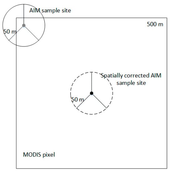
Figure 1.
An Assessment, Inventory, and Monitoring (AIM) sample site (solid line) is off center from the center of a Moderate-Resolution Imaging Spectroradiometer (MODIS) pixel. After relocating the sample site, the spatially corrected AIM sample site (dotted line) is at the center of a MODIS pixel.
2.3. Missing Volumetric Information
Soil elevation is a key factor to represent the land surface conditions, especially in areas with wind erosion [26]. Unlike measuring dust flux, soil elevation reflects the spatial distribution of sediment erosion and deposition [12]. Several field techniques have been created to observe and monitor sediment movements, such as sediment traps [27], erosion pins [28], and erosion bridges [29]. Field observation is not only labor intensive and expensive but also highly depends on the distribution and number of samples. It also misses the volumetric information of some important landforms of wind erosion research, such as dunes.
One of the drone-based remote sensing products is the dense point cloud, which is similar to the point cloud of LiDAR. The dense point cloud not only contains spectral information on land cover but also volumetric information of the land surface. Therefore, a dense point cloud can generate a 3D classification map having one or more land cover classes. The point cloud has been widely used to map the landslide displacement [30], sediment connectivity [31], modeling vegetation height [6], and to estimate the biomass of vegetation [8]. The goal of this experiment is to construct a complete bare ground DTM, which can be used to analyze the soil elevation after erosion, from the point cloud.
2.4. Unidirectional View
The bare soil gap size (the length of a gap with bare soil between two plants), canopy size, and vegetation height are important indicators to study how wind erosion impacts the land surface and vegetation community [32]. Although those indicators can be easily measured by field measurement, the measurements only represent the information in one direction but miss the information in other directions [33]. In research on wind erosion, those indicators strongly vary in different directions. For example, the shrub or grass ecotone may have a banded or street structure along with the prevailing wind direction, respectively [34].
Drone-based remote sensing imagery records spatially continuous information, which allows for observing the details of land cover in an omnidirectional view. This property of drone-based remote sensing can also reproduce measurements in directions that may not have been seen as useful in the original measurement scheme. For example, the directional property describes if a feature has uniformity or not in all orientations. In research on wind erosion, it is an important measurement to represent how the severity of wind erosion impacts the vegetation community and bare ground in different directions [9,34]. The directional property was calculated by a geostatistical measure, “connectivity,” which assesses the probability that adjacent pixels will belong to the same type. The connectivity of bare soil and vegetation in all directions can evaluate the directional influence of wind erosion and determine the direction that has the most severe wind erosion [9]. The goal of this experiment is to compute connectivity based on drone-based remote sensing products and evaluate the directional property of land covers under wind erosion.
2.5. Spatially Inexplicit Input
An ecological model with spatially explicit input has become popular with advancements in computing power [10,35,36]. In research on wind erosion, the major advantage of an ecological model with spatially explicit input is to provide details of land surface changes, biological processes, and the interaction between biotic and abiotic variables at a fine scale [37]. With a spatially explicit input, the model can incorporate complex mathematical and physical equations in the calculation, which was ignored or used as a statistic process to alter in the model with spatially implicit input [10]. Traditionally, in order to mimic the spatially explicit input, interpolation and/or simulation based on the selective samples with spatially explicit behavior were used as the input [38], but none of them are the true spatially explicit input, which affects the performance of the model and the quality of the model’s results.
Drone-based remote sensing can provide the potential input of the ecological models. For example, the WEMO model is a physical model to simulate the impact of aeolian transport on the shrub‒grass mixed vegetation community [39]. This model used the distribution of scaled height, which is the ratio of bare soil gap size to plant height, as the input to describe the land surface conditions. In the past, an exponential function was used to interpolate the scaled height derived from field data to make the distribution as the input. However, the distribution of scaled height can be directly retrieved from the drone-based remote sensing product as the input to the WEMO model. The goal of this experiment is to use the spatially explicit input from the drone-based remote sensing products to run the WEMO model and to compare the results to the field observations.
3. Data and Possible Applications
3.1. Study Area
The study area is the Nutrient Effects of Aeolian Transport (NEAT) site at the Jornada Experimental Range (JER), New Mexico (32°56′ N, 106°75′ W). The NEAT site was established in 2004 to monitor and detect the impacts of wind erosion on the landscape and vegetation community. There are three blocks in the NEAT site and each block has five treatments. All blocks and treatments are aligned parallel to the prevailing wind, which is from the southwest. Each block is 2.5 ha and each treatment is 0.25 ha. There is a 25-m buffer zone between treatments to minimize the interference (wind-blown soil nutrients) between them. The treatments are divided into 25 × 50 m upwind areas and 25 × 50 m downwind areas. In the upwind areas, grasses were manually removed from 100% to 0% (from Treatment 4 to Treatment Control) of its original cover in 2004 and have been maintained at similar levels since 2004. The details of the NEAT site can be found in Zhang [6]. In this paper, Block 3 was used as the study area. The visualized pattern of Block 3 and the treatments can be found in Figure 2.
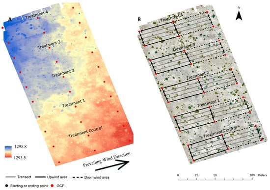
Figure 2.
The digital surface model (DSM) and orthomosaics (A,B) [6] of Block 3 based on the structure from motion (SfM) models. The images were produced by using photos taken in the summer of 2017 using a Dà-Jiāng Innovations (DJI) camera.
3.2. Data Preparation
The image was obtained by a DJI Phantom 4 equipped with its own 4K camera (Dà-Jiāng Innovations Science and Technology Co., Shenzhen, China) in the summer of 2017. DroneDeploy V2.6 (DroneDeploy, San Francisco, CA, USA) was used to initially set up (e.g., flight height and speed) and control the DJI Phantom 4 drone during the flight. The drone was flown twice for a block in different orientations (i.e., north‒south and east‒west) following a “lawnmower” moving pattern to acquire structural information from different aspects. The sidelap of DJI 4K image was set to 70%, which is sufficient to build SfM models of vegetation and landscape. The details about the drone and camera are in Table 1.

Table 1.
The specifications of the drones and the cameras.
The images were processed using a commercial SfM software (PhotoScan V1.2.5, Agisoft LLC, St. Petersburg, Russia). There are four general steps of SfM image processing: (1) photo alignment and sparse point cloud building, (2) Ground control points (GCPs) identification and sparse point cloud optimization, (3) dense point cloud building, and (4) construction of orthomosaic and DSM. The details of processing the imagery can be found in Zhang [6]. The average point density for the dense cloud was 1220 points/m2 for DJI 4K camera. The DJI 4K image resulted in 7 mm and 2.8 cm resolution for orthomosaics and DSMs, respectively.
To assess the spatial accuracy of orthomosaics and DSMs, the spatial root mean square error (RMSE) and spatial mean error (ME) were calculated in the sparse cloud (Table 2). The average RMSE and ME represent the error between the surveyed coordinates of the GCPs in the field and coordinates of those in the sparse cloud model across Block 3. They represent the accuracy of the orthomosaic and the DSM, which were derived from the sparse cloud model.
Table 2.
Evaluation of the accuracies of SfM models based on DJI 4K cameras. X represents longitude, Y represents latitude, and Z represents altitude. Spatial root mean square error (RMSE) and spatial mean error (ME) are between the surveyed coordinates of the ground control points (GCPs) in the field and coordinates of those in the sparse cloud model.
After the orthomosaic and DSM were made, the classification map was produced by an unsupervised classification method, K-means. The algorithm of K-means [40] was based on Tou and Gonzalez [41] and the code was written in IDL 8.5 (L3Harris Technologies, Melbourne, FL, USA). The number of classes is four (grass, shrub, bare soil, and other), the maximum iteration is 20 times, and the minimum change threshold is 0.1. The vegetation layer has used the bare soil mosaic from the classification map to mask the DSM [42]. The vegetation layer is a DSM, which only contains the height information of the canopy. The process was done by ENVI 5.3 (L3Harris Technologies, Melbourne, FL, USA).
3.3. Possible Applications
3.3.1. Provide a Reliable and Valid Sample Set
To simulate the impact of sample size on the quality of sampling, 1000 transect lines, which are along the main axis (the prevailing wind direction) of Treatment 3 of Block 3, are evenly distributed on the classification map and vegetation layer. There is only a 5-cm gap between transect lines and the length of every transect line is 100 m. On each transect, three important wind erosion-related indicators (vegetation cover, plant height, and bare soil gap size) were measured. Vegetation cover was measured by using the line‒point intercept (LPI) method on classification map [13], which recorded the land cover types (i.e., soil, shrub, and grass) at 1-m intervals on the transect line. Therefore, the vegetation cover is the number of shrub and grass records divided by 100. Bare soil gap size, which is measured on classification map, is the length of the gap with bare soil between two plants on the transect line, which is the number of contiguous pixels of bare soil in the transect line times pixel size. Plant height, which is measured on the vegetation layer, is the difference between the largest and the smallest pixel value on the intersection of the transect line and each canopy cluster on the vegetation layer. In each transect line, the averaged values of bare soil gap size and plant height were calculated.
The assumption that the large sample set has a better estimate than the small sample set was tested. Six transect lines, equal distances (7.5 m) from each other, were measured. The statistics (e.g., mean, standard deviation, the confidence interval of mean, and the confidence interval of standard deviation) of the six transect lines and 1000 transect lines were compared.
Although 1000 evenly distributed samples have already increased the sample size, those samples, like the six evenly distributed samples, are highly spatially autocorrelated. Therefore, a method to increase the sample size by using drone-based imagery was designed. Six transect lines were randomly bootstrapped from 1000 transect lines and 1000 draws were made. The mean of six transect lines for each indicator represents the value of one draw. Using this bootstrapping method, which is drawing a subset of samples randomly from a set of samples with replacement, the number of samples in the sample pool is about 1.37 × 10¹⁵, which confirms the basic assumption of sampling: the data pool has a nearly infinite sample size.
For this experiment, the tool in the spatial analyst extension of ArcGIS Desktop 10.8 (ESRI, Redlands, CA, USA) was used to extract the pixel value of the classification map and vegetation layer on the transect line. Python 3.6 with the Geospatial Data Abstraction Library (GDAL) 3.0.1 package [43] was used to implement the calculations for bare soil gap size, plant height, and vegetation cover; generate the random selection of transect lines; and compute the statistic of 1000 random draws for each variable.
3.3.2. Mitigating the Spatial Offset
To simulate the displacement of the field sample from the pixel center, a MODIS image tile (MCD43A4.A2017204.h09v05.006.2017213033355) that contains both Block 3 of NEAT sites and one AIM sample site (#13497) was used for this experiment. The AIM sample can be downloaded from the Landscape Approach Data Portal, https://landscape.blm.gov/geoportal. The drone-based imagery of Block 3 captured the center of this MODIS pixel. The AIM sample site (#13497) is at the upper left corner of one MODIS pixel. The field measurement of the AIM sample site was conducted at the same time as the drone-based remote sensing work in the summer of 2017. For the AIM sample, the bare soil was used as the bare soil cover and total foliar was used as the vegetation cover.
To measure the vegetation cover and bare soil cover at the center of the MODIS pixel, the configuration of the AIM sample site, which was widely used in land management, was mimicked on the classification map. Three 50-m transect lines were created in the direction of 0°, 120°, and 240° at the central location of the MODIS pixel. Then, vegetation cover and bare soil cover were measured by using the LPI method [13], which recorded the land cover types (i.e., soil, shrub, and grass) at 1-m intervals on the transect line. Therefore, the vegetation cover or bare soil cover of one transect line is the number of shrub and grass records or bare soil records divided by 50. Last, the mean vegetation cover and bare soil cover of all three transect lines were calculated. Python 3.6 with Geospatial Data Abstraction Library (GDAL) 3.0.1 package [43] was used to perform the calculations for vegetation and soil cover.
To assess the abundance of vegetation and soil in one MODIS pixel, a spectral unmixing algorithm (SMA) was used to extract the percentage of green vegetation, non-photosynthetic vegetation, and soil at the sub-pixel level. The abundance of green vegetation and non-photosynthetic vegetation was combined with the vegetation cover. The abundance of soil represents the bare soil cover. The spectral library used in this experiment was derived from a combination of field measurements in Savanna [44]. The code of SMA was based on Campbell and Wynne [45] and was written in IDL 8.5.
3.3.3. Soil Elevation
The point cloud is a direct product of drone-based remote sensing. The point cloud not only contains the spectral information of land cover but also the volumetric information of land surface; therefore, a classification method, which is based on the slope of the initial terrain model, was used to distinguish the on-ground object (i.e., vegetation) [46,47]. The classification method has three parameters: max angle, max distance, and cell size. Cell size determines the largest grid of on-ground objects, such as vegetation, but not containing any ground point in the scene. Max angle determines the maximum slope of the ground in the scene. Max distance determines the maximum distance of maximum variation in Z of ground inside the cell size in the scene. The cell size was set to 0.4 m to filter the litter, the max angle to 3°, and the max distance to 0.1 m. Then, a DSM with two classes (bare ground and vegetation) was created with a 2.8 cm spatial resolution. The bare ground feature was selected and the vegetation feature was removed. To fill in those holes (vegetation removal), the DSM raster of bare ground was vectorized first (Figure 3). Then, a fitted interpolation method, which is the natural neighbor interpolation method [48,49], was used to interpolate the holes of the feature layer of bare ground to make a DTM of bare ground (Figure 3).
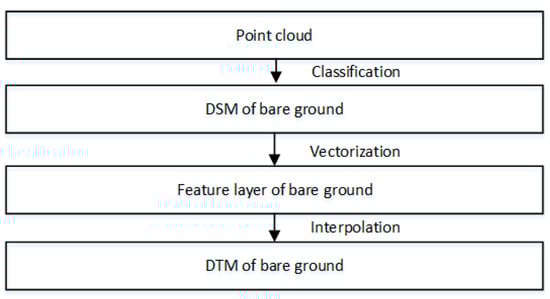
Figure 3.
The workflow of creating a digital terrain model (DTM) raster of bare ground.
To quantitively evaluate the surface height, 500 transect lines were made perpendicular to the prevailing wind direction to measure the pixel value of DTM. The surface height was measured by using the LPI method [13], as in Section 3.3.1 (it recorded the pixel value at 0.1-m intervals on the transect line). This experiment was conducted on the downwind area (which started from the centerline between upwind and downwind area) of Treatment 4 and Treatment Control of Block 3. Block 3 has a relatively flat terrain and the slope of Block 3 is 0.5° from northwest to southeast. Because of that, the relative altitude was used to represent the soil elevation in the different treatments. The mean of the relative altitude on the centerline was marked as 0 m for each treatment. The altitude of each pixel should be subtracted from the mean of the altitude on the centerline to get the relative altitude.
PhotoScan V1.2.5 was used to process the classification of point cloud and the creation of DSM of bare ground. The conversion tool in ArcGIS 10.8 was used to convert the DSM raster of bare soil to a point feature and the Spatial Analyst extension to make an interpolated surface (DTM) of bare ground.
3.3.4. Directional Property of Landscape
Connectivity represents the continuous property of patches along with one direction at a landscape scale. For a classified raster image, a connectivity C can be defined as:
where represents the vector with lag distance , n is the number of successive pixels along in an image, and is a class indicator that equals 1 for pixels that belong to the class of interest and 0 for the other [9]. For example, if “shrub” is the class of interest, then pixels that are classified as “shrub” are given a value of 1, and all other pixels are given a value of 0. In practice, the decrease in connectivity with lag distance approximates an exponential decay function, which is:
where is denoted as the connectivity when is equal to 0 and α represents the maximum lag distance in all directions, which is similar to the “range” of the traditional variograms. In this experiment, the maximum lag distance (α) of each pixel in 360° direction with a 2° interval was calculated [9].
A 20 m × 20 m plot in the upwind area of Treatment 3 and Treatment 1 was selected to calculate the connectivity of vegetation (the classes of shrub and grass) and soil (the class of bare soil) on the classification map. The code of connectivity was written in IDL 8.5.
3.3.5. Spatially Explicit Input
WEMO uses a size distribution of erodible gaps between plants, instead of lateral cover, to describe the distribution of shear stress at the surface. Based on the research of Vest et al. [50], Lancaster et al. [51], Li et al. [52], and Mayaud et al. [53], the WEMO model performed better than the traditional shear stress partitioning approaches. A major advantage of this model is that the primary input variables can be obtained by standard field methods [13] or orthophotography techniques [17]. In this experiment, two different methods were used to describe the distribution of shear stress as the inputs of the WEMO model: one is to use an exponential function to reconstruct a distribution based on the field measurement, the other is to directly measure on the drone-based image to build a distribution.
In the following equation, scaled height x represents the bare soil gap size in units of plant height. Horizontal flux () at a scaled height (x) in the shear stress wake zone is calculated as per Gillette and Chen [54]:
where A is a best-fit constant (0.026), ρ is the density of air (0.00129 g/cm3), g is the acceleration due to gravity (980 cm/s2), and is the threshold of wind shear velocity of the unvegetated soil [52,55], which is 25 cm/s at the experimental sites.
Pd is the probability that any point in the reduced shear stress zone is at a certain distance from the nearest upwind plant in units of plant height. Traditionally, it is estimated as an exponential function [9] with a decay constant, which equals to the estimated median weighted average gap size divided by estimated plant height from the field measurement. In this experiment, Pd was also obtained by using the methods in Section 3.3.1 on the drone-based imagery. The horizontal flux of the whole shear stress wake zone at a specific wind shear velocity () is the sum of for all gap lengths (x), weighted by Pd such that:
where C is the estimated vegetation cover (it was obtained by using the methods in Section 3.3.1 on the drone-based imagery). To calculate the total horizontal flux (Q), is summed for all wind shear velocities () weighted by the probability distribution of wind shear velocity , such that:
In this model, is a constant distribution, which is derived from a three-year (2006–2008) record of wind speed measured at 5-min intervals at the headquarters of JER (Figure 4).
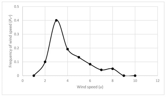
Figure 4.
The probability distribution of the wind speed (u) measured at the headquarters of JER [38].
For each treatment, 500 evenly distributed transect lines were created to measure plant height, bare soil gap size, and vegetation cover in the upwind area of each treatment by using the same method in Section 3.3.1 on the classification map and vegetation layer. The measurement of plant height and bare soil gap size constructed Pd and the measurement of vegetation cover is C in the previous equations. The code of the WEMO model was written in Python 3.6.
4. Results and Discussion
4.1. Provide a Reliable and Valid Sample Set
The means of the vegetation cover, bare soil gap size, and plant height based on six evenly distributed transect lines are similar to the means based on 1000 evenly distributed transect lines (Table 3). However, the standard deviations of vegetation cover, bare soil gap size, and plant height based on six evenly distributed transect lines are larger than the standard deviations based on 1000 evenly distributed transect, which shows that the small sample set has more variation than the large sample set (Table 3 and Figure 5A,C,E). The confidence intervals of the mean and the confidence intervals of the standard deviation of vegetation cover, bare soil gap size, and plant height based on six evenly distributed transect lines are, at least, twice as large as the confidence intervals of the mean and the confidence intervals of the standard deviation based on 1000 evenly distributed transects, which shows that the small sample set involves more uncertainty than the large sample set (Table 3).
Table 3.
The mean, standard deviation, confidence interval of mean, and confidence interval of standard deviation of 6 and 1000 evenly distributed transect lines and 1000 draws for vegetation cover, bare soil gap size, and plant height.
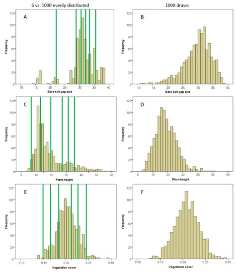
Figure 5.
Histograms exhibit the mean of bare soil gap size, plant height, and vegetation cover for six and 1000 evenly distributed transect lines (A,C,E: green lines represent six evenly distributed transect lines and yellow lines represent 1000 evenly distributed transect lines) and 1000 draws (B,D,F) of Treatment 3 (75% grass removal).
Vegetation covers show the nearly normal distribution of 1000 transect lines and 1000 draws (Figure 5B,D,F). The mean of 1000 transect lines and 1000 draws are the same, but the standard deviation of 1000 draws is smaller than 1000 transect lines. The confidence interval of the mean of 1000 transect lines is five times larger than with 1000 draws and the confidence interval of the standard deviation of 1000 transect lines is four times larger than with 1000 draws (Table 3). The average bare soil gap size of transect lines shows the slightly skewed distribution of 1000 draws with a mean of 3293.53 cm and a standard deviation of 798.725 cm (Figure 5B,D,F). The confidence interval of the mean and standard deviation of 1000 transect lines is twice as large as with 1000 draws (Table 3). Average plant height in transect lines shows a highly skewed distribution of 1000 draws with a mean of 18.90 cm and a standard deviation of 7.19 cm (Figure 5B,D,F). The confidence interval of the mean of 1000 transect lines is four times larger than with 1000 draws and the confidence interval of the standard deviation of 1000 transect lines is twice as large as with 1000 draws (Table 3).
Providing a large sample has the advantage of reducing confidence intervals, particularly for the confidence interval for the standard deviation, because the magnitude of the confidence interval for the standard deviation decreases more slowly with the number of degrees of freedom than that for the mean. This means that a larger sample size is required to estimate the confidence interval for the variance (as a proportion of variance) than is required for the estimation of the confidence interval of the mean (as a proportion of the mean). Further, the results from bootstrapped resampling indicate that a priori unknown biases potentially exist (as indicated by the skewed distributions in Figure 5, right column) after the removal of spatial autocorrelation. When using only evenly distributed transects (six or 1000), the biases that depended on the land cover were not found. In this case, the drone-based imagery not only provides a large sample set but also gives a chance to resample the large sample set and provide a reliable and valid sample set.
4.2. Mitigating the Spatial Offset
The actual displacement from the AIM sample site to the center of the MODIS pixel is 323.5 m. The bare soil cover and vegetation cover from the drone-based estimate (remeasured on the drone imagery using the LPI method) is 79.5% and 20.5% (Table 4), respectively, which are less different from the SMA result of the MODIS pixel compared to the field measurement (71.9% for bare soil cover and 28.3% for vegetation cover). That is because the field measurement contains information not only on the MODIS pixel that covers the center of the AIM sample site but also on three adjacent MODIS pixels (upper, upper left, and left).
Table 4.
The bare soil cover and vegetation cover from field measurement, drone-based estimate, and MODIS pixel.
Those differences should not be ignored and may strongly affect the accuracy of any follow-up analysis and computation. In some studies [20,21], the prediction errors (underpredicted high value and overpredicted low value) came from the spatial offset between the field sample site and the pixel of remote sensing products. Although there is an existing method that uses a linear equation to correct the error from the spatial offset [22], this method assumes that all samples must have the same spatial characteristics. It is not suitable for research on a continental or global scale since the samples were from different ecoregions and have different spatial characteristics. Moreover, the linear correction method has a good performance for a relatively small pixel size such as Landsat or Sentinel. However, for relatively large pixel sizes, such as in MODIS, the linear correction method did not perform well [7]. In this case, the drone-based imagery is a good supplemental material for the correction of spatial displacement.
4.3. Soil Elevation
The bare ground DTM of Treatment 4 has an obviously increasing trend of relative altitude along with the prevailing wind direction but Treatment Control does not show that increasing trend from the centerline between the upwind and downwind areas (Figure 6). In Treatment 4, the upwind area has no grass cover, which caused strong wind erosion (soil loss). The impact of strong wind erosion extended to the front region of the downwind area (0–10 m from the centerline). The blown-up soil particles deposited on the area at 10 m of the centerline and became a dune-shape landscape. Moreover, the deposition of soil particles also brought nutrients for the grasses to accelerate their growth. The grass community can trap more blown-up soil, which also accelerated the formation of the dune-shape landscape. Due to that, the increasing trend of relative altitude along with the prevailing wind direction was created. In Treatment Control, the upwind area has no grass removal and the wind erosion is uniform, along with the prevailing wind direction; therefore, relative altitude does not have a clear tendency.
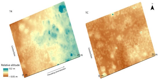
Figure 6.
The relative altitude of bare ground DTM of Treatment 4 (T4) and Treatment Control (TC) downwind areas.
From the analysis of 500 transect lines (Figure 7), the range of relative altitude in Treatment Control is from 0.020 to 0.032 m and the range of relative altitude in Treatment 4 is from 0.021 to 0.152 m, which is much larger than Treatment Control. The curve of Treatment 4 shows that the slope between 12.5 m to 17.5 m is the largest because that area has the most accumulation of blown-up soil particles, which became a band structure [34]. The curve of Treatment Control shows a slight variation. There is a trough from 7.5 m to 10 m because the vegetation distribution in that area varies a lot. In this case, drone-based DTM provides an opportunity for studying the landform in a 3D view.
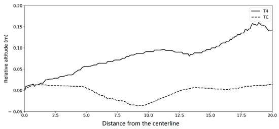
Figure 7.
The mean relative altitude of 500 transect lines on the downwind areas of Treatment 4 (T4) and Treatment Control (TC).
4.4. Directional Property of Landscape
In Treatment 3, the average bare soil patches are larger than the average vegetation clusters and both exhibit marked anisotropy (Figure 8A,C). The direction of vegetation clusters is aligned with the prevailing wind direction, suggesting a role of the wind in shaping the vegetation clusters. It also means that the vegetation community has more connectivity in the direction of the prevailing wind. The bare soil patches have more connectivity in the perpendicular direction of the prevailing wind. In Treatment 1, the average bare soil patches are close to the average vegetation clusters. The bare soil patches exhibit anisotropy but the vegetation clusters exhibit isotropy (Figure 8B,D). The direction of soil patches is perpendicular to the direction of the prevailing wind, with a 10° difference. The decay curves of connectivity of bare soil patches and vegetation clusters follow an exponential function. The bare soil patches have more connectivity than the vegetation clusters because bare soil is the dominant land cover in the study area, as can be seen in Figure 2.
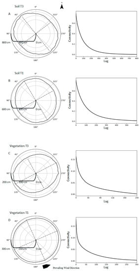
Figure 8.
Polar plots of the average size of inter-plant gaps and vegetation patches using the method of McGlynn and Okin [9] for the upwind portion of Treatment 3 (75% grass removal) and Treatment 1 (25% grass removal) (left column). The decay curves of connectivity of interplant gaps and vegetation patches for the upwind portion of Treatment 3 and Treatment Control 1 (right column). The directional property of Treatment 3 (A,C); the directional property of Treatment 1 (B,D). This figure was revised from Zhang et al. [17].
In Treatment 3, the shape of bare patches, perhaps due to their recent genesis, is different from that described by McGlynn and Okin [9] for an established shrub dune. The orientation of well-developed bare soil patches is parallel to the direction of the prevailing wind. In Treatment 1, the result is the same as in Okin et al. [34,56], in which the size of bare soil patches and vegetation clusters are close in an established shrub‒grass mixed community. The connectivity, in this experiment, only represents the soil patches and vegetation clusters (shrub and grass). In the future, this method may be employed to detect the differences between grass and shrub, which could reveal the details of the competition of shrub and grass during wind erosion. In this case, drone-based imagery is a good way to conduct multidirectional research.
4.5. Spatially Explicit Input
The daily dust fluxes computed using drone-based imagery are in the range of the field experiments performed using a wind tunnel [57]. The dust flux of Treatment 4 (2.8 g/cm/day) is much higher than for the remaining treatments because the percentage of grass removal in the upwind area of Treatment 4 is higher than for the remaining treatments. The median, first quartile, and third quartile of dust flux computed using drone-based imagery have a decreasing gradient from Treatment 4 to Treatment Control (Figure 9). However, there is no obvious decreasing gradient of dust flux when using field measurements from Treatment 4 to Treatment Control for the median, first quartile, and third quartile. The median of Treatment 1 is greater than the rest and the median of Treatment 2 is smaller than the rest, which contradicts the observations from the wind tunnel [57]. Moreover, the medians of Treatment 4 and Treatment 3 are much smaller than the observations from wind erosion [57].
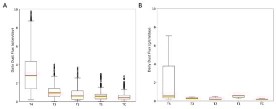
Figure 9.
The box plot of daily dust flux (g/cm/day) was computed by using the WEMO model on the upwind area of Treatment 4-Treatment Control (T4-TC, 100% grass removal-0% grass removal). The input of WEMO is from the drone-based estimate (500 transect lines, (A) and field measurement (three transect lines, (B). The yellow mark represents the median value of dust flux.
From the results, the WEMO model using spatially explicit input shows an obvious decreasing trend from Treatment 4 to Treatment Control. In this case, the spatially explicit input, somehow, reflects the details of the land surface condition compared to the field data. In the future, more models for the research of wind erosion, such as the Vegetation and Sediment Transport (ViSTA) model [53] and Ecotone‒WEMO model [38], can be tested by using the spatially explicit input.
5. Conclusions
This paper sheds light on the possible applications of drone-based remote sensing in research on wind erosion, which was inspired by the difficulties of field data collection. Through the five experiments, drone-based products (i.e., dense point cloud, orthomosaic imagery, and DSM) were shown to be useful for wind erosion research in drylands for the following reasons: a reliable and valid sample set based on bootstrapping resampling; the displacement of field sample site eases the attenuation bias between the field measurement and remote sensing product; the point cloud built DTM shows the pattern of soil distribution and the trend of soil elevation; the land cover under wind erosion condition has an anisotropic pattern; and the WEMO model produces significant results after using the spatially explicit input. At present, drone-based imagery has been suggested as a means to complete difficult fieldwork in remote areas or during harsh weather conditions. For wind erosion research in drylands, the drone-based remote sensing product should be used as a complement to field measurement.
Author Contributions
Conceptualization, J.Z., W.G., and G.S.O.; methodology, J.Z.; software, J.Z. and B.Z.; validation, J.Z. and B.Z.; formal analysis, J.Z.; investigation, J.Z.; resources, J.Z. and G.S.O.; data curation, J.Z. and G.S.O. writing—original draft preparation, J.Z.; writing—review and editing, J.Z., G.S.O., and W.G.; visualization, J.Z.; supervision, J.Z.; project administration, J.Z. and G.S.O.; funding acquisition, W.G. All authors have read and agreed to the published version of the manuscript.
Funding
This study was supported by the National Natural Science Foundation of China (42071124), the 2nd Tibetan Plateau Scientific Expedition and Research (2019QZKK0101), the Strategic Priority Research Program of Chinese Academy of Sciences (XDB40020200), the Fundamental Research Funds for the Central Universities (XZY012019008), and the State Key Laboratory of Loess and Quaternary Geology (SKLLQG1809).
Institutional Review Board Statement
Not applicable.
Informed Consent Statement
Not applicable.
Data Availability Statement
The data presented in this study are available only on request from the first author. The data are not publicly available due to the policy of UCLA.
Conflicts of Interest
The authors declare no conflict of interest.
References
- Webb, N.P.; Okin, G.S.; Brown, S. The effect of roughness elements on wind erosion: The importance of surface shear stress distribution. J. Geophys. Res. Atmos. 2014, 119, 6066–6084. [Google Scholar] [CrossRef]
- Shao, Y. Physics and Modelling of Wind Erosion; Springer: Amsterdam, The Netherlands, 2000. [Google Scholar]
- Belnap, J.; Gillette, D.A. Vulnerability of desert biological soil crusts to wind erosion: The influences of crust development, soil texture, and disturbance. J. Arid Environ. 1998, 39, 133–142. [Google Scholar] [CrossRef]
- Bhattachan, A.; Okin, G.S.; Zhang, J.; Vimal, S.; Lettenmaier, D.P. Characterizing the role of wind and dust in traffic accidents in California. GeoHealth 2019, 3, 328–336. [Google Scholar] [CrossRef] [PubMed]
- Okin, G.S.; Sala, O.E.; Vivoni, E.R.; Zhang, J.; Bhattachan, A. The interactive role of wind and water in functioning of drylands: What does the future hold? Bioscience 2018, 68, 670–677. [Google Scholar] [CrossRef]
- Zhang, J. Multi-Scale Vegetation-Aeolian Transport Interaction in Drylands: Remote Sensing and Modeling; UCLA: Los Angeles, CA, USA, 2019. [Google Scholar]
- Hogland, J.; Affleck, D.L. Mitigating the impact of field and image registration errors through spatial aggregation. Remote Sens. 2019, 11, 222. [Google Scholar] [CrossRef]
- Cunliffe, A.M.; Brazier, R.E.; Anderson, K. Ultra-fine grain landscape-scale quantification of dryland vegetation structure with drone-acquired structure-from-motion photogrammetry. Remote Sens. Environ. 2016, 183, 129–143. [Google Scholar] [CrossRef]
- McGlynn, I.O.; Okin, G.S. Characterization of shrub distribution using high spatial resolution remote sensing: Ecosystem implications for a former Chihuahuan Desert grassland. Remote Sens. Environ. 2006, 101, 554–566. [Google Scholar] [CrossRef]
- DeAngelis, D.L.; Yurek, S. Spatially explicit modeling in ecology: A review. Ecosystems 2017, 20, 284–300. [Google Scholar] [CrossRef]
- Daftry, S.; Hoppe, C.; Bischof, H. Building with drones: Accurate 3d facade reconstruction using mavs. In Proceedings of the 2015 IEEE International Conference on Robotics and Automation (ICRA), Seattle, DC, USA, 26–30 May 2015; pp. 3487–3494. [Google Scholar]
- Gillan, J.K.; Karl, J.W.; Elaksher, A.; Duniway, M.C. Fine-Resolution Repeat Topographic Surveying of Dryland Landscapes Using UAS-Based Structure-from-Motion Photogrammetry: Assessing Accuracy and Precision against Traditional Ground-Based Erosion Measurements. Remote Sens. 2017, 9, 437. [Google Scholar] [CrossRef]
- Herrick, J.E.; Van Zee, J.W.; Havstad, K.M.; Burkett, L.M.; Whitford, W.G.; Bestelmeyer, B.T.; Melgoza, A.; Pellant, M.; Pyke, D.A.; Remmenga, M.D. Monitoring manual for grassland, shrubland and savanna ecosystems. In Volume I: Core Methods; USDA-ARS Jornada Experimental Range: Las Cruces, NM, USA, 2005. [Google Scholar]
- Webb, N.P.; Chappell, A.; Edwards, B.L.; McCord, S.E.; Van Zee, J.W.; Cooper, B.F.; Courtright, E.M.; Duniway, M.C.; Sharratt, B.; Tedela, N. Reducing sampling uncertainty in aeolian research to improve change detection. J. Geophys. Res. Earth Surf. 2019, 124, 1366–1377. [Google Scholar] [CrossRef]
- Karl, J.W.; McCord, S.E.; Hadley, B.C. A comparison of cover calculation techniques for relating point-intercept vegetation sampling to remote sensing imagery. Ecol. Indic. 2017, 73, 156–165. [Google Scholar] [CrossRef]
- Duniway, M.C.; Karl, J.W.; Schrader, S.; Baquera, N.; Herrick, J.E. Rangeland and pasture monitoring: An approach to interpretation of high-resolution imagery focused on observer calibration for repeatability. Environ. Monit. Assess. 2012, 184, 3789–3804. [Google Scholar] [CrossRef] [PubMed]
- Zhang, J.; Okin, G.S.; Zhou, B.; Karl, J.W. Quantifying rangeland indicators from drone-based remote sensing images: Experiments and applications. Ecosphere 2021, in press. [Google Scholar]
- Webb, N.P.; Van Zee, J.W.; Karl, J.W.; Herrick, J.E.; Courtright, E.M.; Billings, B.J.; Boyd, R.; Chappell, A.; Duniway, M.C.; Derner, J.D. Enhancing wind erosion monitoring and assessment for US rangelands. Rangelands 2017, 39, 85–96. [Google Scholar] [CrossRef]
- McCord, S.E.; Buenemann, M.; Karl, J.W.; Browning, D.M.; Hadley, B.C. Integrating Remotely Sensed Imagery and Existing Multiscale Field Data to Derive Rangeland Indicators: Application of Bayesian Additive Regression Trees. Rangel. Ecol. Manag. 2017, 70, 644–655. [Google Scholar] [CrossRef]
- Zhou, B.; Okin, G.S.; Zhang, J. Leveraging Google Earth Engine (GEE) and machine learning algorithms to incorporate in situ measurement from different times for rangelands monitoring. Remote Sens. Environ. 2020, 236, 111521. [Google Scholar] [CrossRef]
- Zhang, J.; Okin, G.S.; Zhou, B. Assimilating optical satellite remote sensing images and field data to predict surface indicators in the Western US: Assessing error in satellite predictions based on large geographical datasets with the use of machine learning. Remote Sens. Environ. 2019, 233, 111382. [Google Scholar] [CrossRef]
- Hogland, J.; Anderson, N. Function modeling improves the efficiency of spatial modeling using big data from remote sensing. Big Data Cogn. Comput. 2017, 1, 3. [Google Scholar] [CrossRef]
- Schmid, J.N. Using Google Earth Engine for Landsat NDVI Time Series Analysis to Indicate the Present Status of Forest Stands. Bachelor’s Thesis, Georg-August-University, Göttingen, Germany, October 2017. [Google Scholar]
- Masinde, C.; Rono, D.; Hahn, M. Estimation of the degree of surface sealing with Sentinel 2 data using building indices. Earth Obs. Geomat. Eng. 2019, 3, 112–119. [Google Scholar]
- Herrick, J.E.; Lessard, V.C.; Spaeth, K.E.; Shaver, P.L.; Dayton, R.S.; Pyke, D.A.; Jolley, L.; Goebel, J.J. National ecosystem assessments supported by scientific and local knowledge. Front. Ecol. Environ. 2010, 8, 403–408. [Google Scholar] [CrossRef]
- Gillan, J.K.; Karl, J.W.; Barger, N.N.; Elaksher, A.; Duniway, M.C. Spatially explicit rangeland erosion monitoring using high-resolution digital aerial imagery. Rangel. Ecol. Manag. 2016, 69, 95–107. [Google Scholar] [CrossRef]
- Nichols, M. Measured sediment yield rates from semiarid rangeland watersheds. Rangel. Ecol. Manag. 2006, 59, 55–62. [Google Scholar] [CrossRef]
- Sirvent, J.; Desir, G.; Gutierrez, M.; Sancho, C.; Benito, G. Erosion rates in badland areas recorded by collectors, erosion pins and profilometer techniques (Ebro Basin, NE-Spain). Geomorphology 1997, 18, 61–75. [Google Scholar] [CrossRef]
- Wilcox, B.; Davenport, D.; Pitlick, J.; Allen, C. Runoff and Erosion from a Rapidly Eroding Pinyon-Juniper Hillslope; Los Alamos National Lab.: Los Alamos, NM, USA, 1996.
- Lucieer, A.; Jong, S.M.d.; Turner, D. Mapping landslide displacements using Structure from Motion (SfM) and image correlation of multi-temporal UAV photography. Prog. Phys. Geogr. 2014, 38, 97–116. [Google Scholar] [CrossRef]
- Estrany, J.; Ruiz, M.; Calsamiglia, A.; Carriquí, M.; García-Comendador, J.; Nadal, M.; Fortesa, J.; López-Tarazón, J.A.; Medrano, H.; Gago, J. Sediment connectivity linked to vegetation using UAVs: High-resolution imagery for ecosystem management. Sci. Total Environ. 2019, 671, 1192–1205. [Google Scholar] [CrossRef]
- Webb, N.P.; Kachergis, E.; Miller, S.W.; McCord, S.E.; Bestelmeyer, B.T.; Brown, J.R.; Chappell, A.; Edwards, B.L.; Herrick, J.E.; Karl, J.W. Indicators and benchmarks for wind erosion monitoring, assessment and management. Ecol. Indic. 2020, 110, 105881. [Google Scholar] [CrossRef]
- Peters, D.P.; Okin, G.S.; Herrick, J.E.; Savoy, H.M.; Anderson, J.P.; Scroggs, S.L.; Zhang, J. Modifying connectivity to promote state change reversal: The importance of geomorphic context and plant–soil feedbacks. Ecology 2020, e03069. [Google Scholar] [CrossRef]
- Okin, G.S.; Moreno-de las Heras, M.; Saco, P.M.; Throop, H.L.; Vivoni, E.R.; Parsons, A.J.; Wainwright, J.; Peters, D.P.C. Connectivity in dryland landscapes: Shifting concepts of spatial interactions. Front. Ecol. Environ. 2015, 13, 20–27. [Google Scholar] [CrossRef]
- Turner, M.G.; Arthaud, G.J.; Engstrom, R.T.; Hejl, S.J.; Liu, J.; Loeb, S.; McKelvey, K. Usefulness of spatially explicit population models in land management. Ecol. Appl. 1995, 5, 12–16. [Google Scholar] [CrossRef]
- Wu, J.; David, J.L. A spatially explicit hierarchical approach to modeling complex ecological systems: Theory and applications. Ecol. Model. 2002, 153, 7–26. [Google Scholar] [CrossRef]
- Dunning, J.B., Jr.; Stewart, D.J.; Danielson, B.J.; Noon, B.R.; Root, T.L.; Lamberson, R.H.; Stevens, E.E. Spatially explicit population models: Current forms and future uses. Ecol. Appl. 1995, 5, 3–11. [Google Scholar] [CrossRef]
- Zhang, J. A new ecological-wind erosion model to simulate the impacts of aeolian transport on dryland vegetation patterns. Acta Ecol. Sin. 2020. [Google Scholar] [CrossRef]
- Okin, G.S. A new model of wind erosion in the presence of vegetation. J. Geophys. Res. Earth 2008, 113, 954. [Google Scholar] [CrossRef]
- Zhang, J.; Zhu, W.; Dong, Y.; Jiang, N.; Pan, Y. A spectral similarity measure based on Changing-Weight Combination Method. Acta Geod. Cartogr. Sin. 2013, 42, 418–424. [Google Scholar]
- Tou, J.T.; Gonzalez, R.C. Pattern Recognition Principles; Addison-Wesley Publishing Company: Boston, MA, USA, 1974. [Google Scholar]
- Gillan, J.K.; Karl, J.W.; Duniway, M.; Elaksher, A. Modeling vegetation heights from high resolution stereo aerial photography: An application for broad-scale rangeland monitoring. J. Environ. Manag. 2014, 144, 226–235. [Google Scholar] [CrossRef]
- Warmerdam, F. The geospatial data abstraction library. In Open Source Approaches in Spatial Data Handling; Springer: Berlin/Heidelberg, Germany, 2008; pp. 87–104. [Google Scholar]
- Meyer, T.; Okin, G.S. Evaluation of spectral unmixing techniques using MODIS in a structurally complex savanna environment for retrieval of green vegetation, nonphotosynthetic vegetation, and soil fractional cover. Remote Sens. Environ. 2015, 161, 122–130. [Google Scholar] [CrossRef]
- Campbell, J.B.; Wynne, R.H. Introduction to Remote Sensing; Guilford Press: New York, NY, USA, 2011. [Google Scholar]
- Jensen, J.L.; Mathews, A.J. Assessment of image-based point cloud products to generate a bare earth surface and estimate canopy heights in a woodland ecosystem. Remote Sens. 2016, 8, 50. [Google Scholar] [CrossRef]
- Dandois, J.P.; Ellis, E.C. High spatial resolution three-dimensional mapping of vegetation spectral dynamics using computer vision. Remote Sens. Environ. 2013, 136, 259–276. [Google Scholar] [CrossRef]
- Hongyue, D.; Junzhe, Z.; Huili, G. Research of DEM quality-precision analysis and system implementation. Sci. Surv. Mapp. 2009, 4, 191–194. [Google Scholar]
- Sibson, R. A brief description of natural neighbour interpolation. In Interpreting Multivariate Data; Barnett, V., Ed.; Wiley: New York, NY, USA, 1981. [Google Scholar]
- Vest, K.R.; Elmore, A.J.; Kaste, J.M.; Okin, G.S.; Li, J.R. Estimating total horizontal aeolian flux within shrub-invaded groundwater-dependent meadows using empirical and mechanistic models. J. Geophys. Res. Earth 2013, 118, 1132–1146. [Google Scholar] [CrossRef]
- Lancaster, N.; Nickling, W.G.; Gillies, J.A. Sand transport by wind on complex surfaces: Field studies in the McMurdo Dry Valleys, Antarctica. J. Geophys. Res. Earth Surf. 2010, 115, 115. [Google Scholar] [CrossRef]
- Li, J.R.; Okin, G.S.; Herrick, J.E.; Belnap, J.; Miller, M.E.; Vest, K.; Draut, A.E. Evaluation of a new model of aeolian transport in the presence of vegetation. J. Geophys. Res. Earth 2013, 118, 288–306. [Google Scholar] [CrossRef]
- Mayaud, J.R.; Bailey, R.M.; Wiggs, G.F. A coupled vegetation/sediment transport model for dryland environments. J. Geophys. Res. Earth Surf. 2017, 122, 875–900. [Google Scholar] [CrossRef]
- Gillette, D.A.; Chen, W. Particle production and aeolian transport from a “supply-limited” source area in the Chihuahuan desert, New Mexico, United States. J. Geophys. Res. Atmos. 2001, 106, 5267–5278. [Google Scholar] [CrossRef]
- Gillette, D.A.; Adams, J.; Endo, A.; Smith, D.; Kihl, R. Threshold velocities for input of soil particles into the air by desert soils. J. Geophys. Res. Ocean. 1980, 85, 5621–5630. [Google Scholar] [CrossRef]
- Alvarez, L.J.; Epstein, H.E.; Li, J.R.; Okin, G.S. Aeolian process effects on vegetation communities in an arid grassland ecosystem. Ecol. Evol. 2012, 2, 809–821. [Google Scholar] [CrossRef]
- Gillette, D.A.; Pitchford, A.M. Sand flux in the northern Chihuahuan Desert, New Mexico, USA, and the influence of mesquite-dominated landscapes. J. Geophys. Res. Earth Surf. 2004, 109. [Google Scholar] [CrossRef]


Publisher’s Note: MDPI stays neutral with regard to jurisdictional claims in published maps and institutional affiliations. |
© 2021 by the authors. Licensee MDPI, Basel, Switzerland. This article is an open access article distributed under the terms and conditions of the Creative Commons Attribution (CC BY) license (http://creativecommons.org/licenses/by/4.0/).