Article

Monitoring Changes to Arctic Vegetation and Glaciers at Ny-Ålesund, Svalbard, Based on Time Series Remote Sensing

1
Lab of Marine Physics and Remote Sensing, First Institute of Oceanography, Ministry of Natural Resources, Qingdao 266061, China
2
National Satellite Ocean Application Service, Ministry of Natural Resources, Beijing 100081, China
*
Author to whom correspondence should be addressed.
Remote Sens. 2021, 13(19), 3845; https://doi.org/10.3390/rs13193845
Submission received: 18 August 2021 / Revised: 11 September 2021 / Accepted: 16 September 2021 / Published: 26 September 2021
(This article belongs to the Special Issue Remote Sensing Monitoring of Arctic Environments)

Abstract

:
Climate change has profoundly affected global ecological security. The most vulnerable region on Earth is the high-latitude Arctic. Identifying the changes in vegetation coverage and glaciers in high-latitude Arctic coastal regions is important for understanding the process and impact of global climate change. Ny-Ålesund, the northern-most human settlement, is typical of these coastal regions and was used as a study site. Vegetation and glacier changes over the past 35 years were studied using time series remote sensing data from Landsat 5/7/8 acquired in 1985, 1989, 2000, 2011, 2015 and 2019. Site survey data in 2019, a digital elevation model from 2009 and meteorological data observed from 1985 to 2019 were also used. The vegetation in the Ny-Ålesund coastal zone showed a trend of declining and then increasing, with a breaking point in 2000. However, the area of vegetation with coverage greater than 30% increased over the whole study period, and the wetland moss area also increased, which may be caused by the accelerated melting of glaciers. Human activities were responsible for the decline in vegetation cover around Ny-Ålesund owing to the construction of the town and airport. Even in areas with vegetation coverage of only 13%, there were at least five species of high-latitude plants. The melting rate of five major glaciers in the study area accelerated, and approximately 82% of the reduction in glacier area occurred after 2000. The elevation of the lowest boundary of the five glaciers increased by 50–70 m. The increase in precipitation and the average annual temperature after 2000 explains the changes in both vegetation coverage and glaciers in the study period.

Graphical Abstract

1. Introduction

Vegetation communities in the Arctic region are extremely vulnerable to major or irreversible changes [1,2] because of their special adaptation to an environment that includes a short growing season, low temperature, low precipitation, lack of soil nutrients and permafrost. Global warming has led to a large decrease in sea ice, glaciers and snow cover worldwide. The Arctic region bears the brunt of these changes, and its warming trend is more pronounced than in other regions of the world [3]. Some studies indicate that the Arctic is experiencing its greatest warming event in the past 50,000 years [4], and the melting of snow and ice will have a profound impact on global ocean circulation and climate [5,6]. Because the Arctic region is highly responsive to global climate change, monitoring changes in vegetation and glaciers in the polar coastal zone is an important way to identify climate change [7,8,9]. The impact of global warming on the polar regions is directly related to their carbon cycle, especially the sequestration of atmospheric greenhouse gases by plants [10]. The rising temperature in the Arctic advances snow melt in spring and increases the time when Arctic vegetation can receive sunlight, which leads to greater primary productivity of Arctic ecosystems and changes the competitive advantage between different vegetation species and communities [11]. Conversely, the melting of glaciers in the Arctic has accelerated under the dual effects of human activities and climate warming, coupled with insufficient precipitation [12].
Ny-Ålesund is located on the Brøggerhalvøya peninsula in northwest Svalbard, which hosts several scientific research stations belonging to the world’s major Arctic research countries. Svalbard is located between 10° to 35° E and 74° to 81° N, halfway between Norway and the North Pole, with a total area of approximately 63,000 km2 [13]. Since the end of the Little Ice Age in the 19th century, the glaciers on Svalbard have been in continuous retreat; in 1985, 60% of the island was covered by glaciers [14]. Every summer, glacial meltwater changes the topography of the coast and provides a source of water for vegetation growth and vegetation coverage changes [7,15].
The distribution of vegetation on Svalbard used to be measured with traditional survey methods [16]. The first vegetation monitoring map based on remote sensing did not appear until 1990 [17]. In 1994, Brossard and Joly [15] used Landsat TM images acquired in 1985 and field survey data to complete a thematic map of the probable occurrence of vegetation types covering the study area. In 1995, [17] applied an unsupervised classification methods based on Landsat images and field survey data to produce a classified vegetation map of the area surrounding Ny-Ålesund. Subsequently, a limited number of studies on land cover and vegetation monitoring based on remote sensing technology have been published [18,19,20], but few have used time series monitoring and analysis of changes in Arctic coastal vegetation and glaciers based on remote sensing for this area.
Observations and research have shown that the temperature in the area surrounding Ny-Ålesund is rising, while snowfall and precipitation have a clear downward trend [21]. The vegetation ecosystems and glaciers in polar regions are highly sensitive to these types of climatic change [22,23]. Ny-Ålesund is the northernmost human settlement on Svalbard. There is no doubt that the dynamics of the vegetation ecosystem, glaciers and climate change will influence the security of this Arctic research hub. The current study used six Landsat satellite remote sensing images covering the past 35 years (1985–2019), combined with field survey data, a digital elevation model and climate observations, to monitor the changes in vegetation and glaciers in Ny-Ålesund and analyze their dynamic characteristics.

2. Study Area and Materials
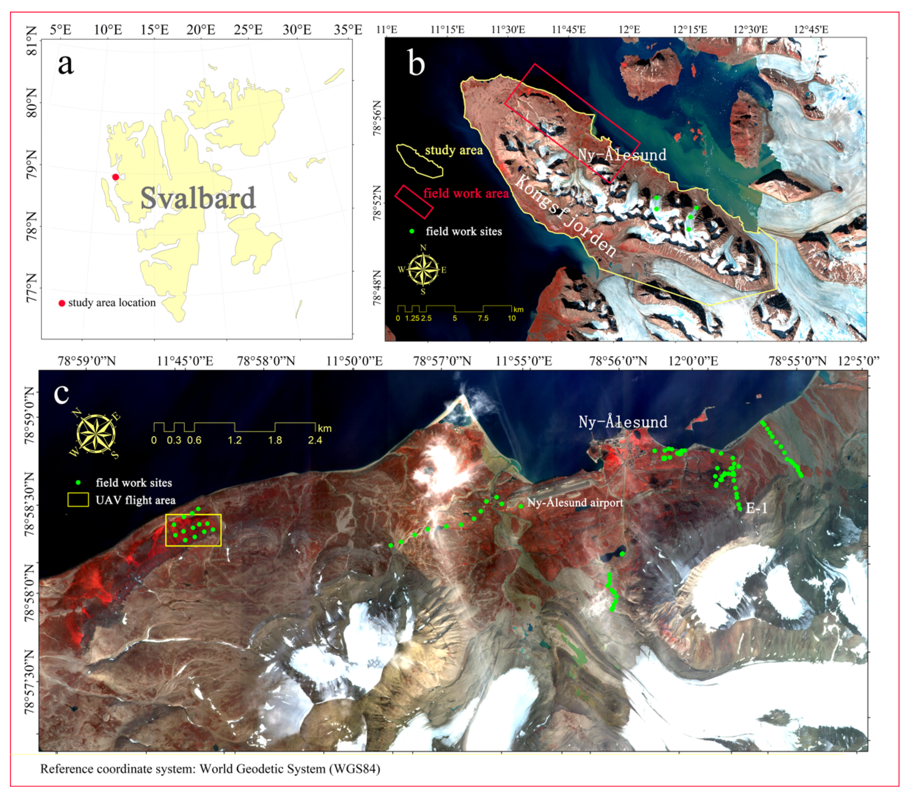
2.1. Study Area

The study area is the Brøgger peninsula (Brøggerhalvøya), including the small town of Ny-Ålesund, in the northwest of the Norwegian Svalbard Islands in the Arctic Ocean, at a latitude and longitude of approximately 78.9°N and 11.9°E (Figure 1). The peninsula where Ny-Ålesund is located runs northwest–southeast and is approximately 30 km long. Because of the influence of alluvial deposition and erosion by glacial meltwater, the peninsula has developed a variety of bedrock, sandy and silty coasts. In contrast to temperate and tropical coastal zones, the polar coastal zone has permafrost below. On the silty coast where there is insufficient sediment, erosive coastlines can form with a cliff-like layer of frozen soil. Thermokarst lakes occur mainly in the sandy coastal zone. These are formed by the difference in specific heat capacity when the permafrost layer melts and water accumulates. The vegetation in this area is mostly herbs that are common on plateaus and in polar regions, with Salix arctica as the only woody vegetation. In the polar regions, owing to the limitations of temperature, light and soil nutrients, the proportion of vegetation cover is generally low, but in the valleys that are fed by glacier meltwater, there are many moss communities with high coverage. The study includes five major glaciers distributed along the peninsula. From the northwest to southeast they are named Vestre Brøggerbreen, Austre Brøggerbreen, Midtre Lovenbreen, Austre Lovenbreen and Pedersenbreen. Glaciers in Svalbard have been experiencing serious reductions in area over the past few decades owing to local and global climate change [24].

2.2. Remote Sensing Data

Landsat series satellite images were chosen as the data source for monitoring change to ensure that the results in different periods were comparable. Landsat images, with a relatively constant spatial resolution of 30 m, have good temporal continuity and suitable image indices (such as NDVI and NDSI) for monitoring vegetation, water bodies and glaciers. To verify the ability of Landsat data to monitor vegetation and glaciers at different spatial resolutions, we also used Gaofen-2 satellite data with a spatial resolution of 4 m and UAV data with a spatial resolution of 3 cm as data sources. The detailed parameters of the remote sensing data are shown in Table 1.
The satellite and UAV remote sensing images in this study had the following characteristics. First, the data covered July and August. Owing to the high latitude of Svalbard, the vegetation growth season only lasts from June to September each year, and vigorous growth occurs only in July and August. Second, the solar altitude angle is low compared with the low and middle latitude regions. The imaging time of Landsat 5 TM and Landsat 7 ETM+ remote sensing images before 2015 was from 11 am to 12 noon local time, so the solar altitude angle at the imaging time was approximately the same, ~30°. However, both the Landsat 8 OLI images in 2019 and the Gaofen-2 images in 2015 had a solar altitude angle of below 20°. The effect of the resulting mountain shadows in the images must be considered for the accurate monitoring of vegetation and glaciers in the study area.
Landsat satellite series were the main data source for large-scale vegetation and glacier distribution monitoring and change analysis. Gaofen-2 images had a high spatial resolution, with four bands including blue (0.45–0.52 μm), green (0.52–0.59 μm), red (0.63–0.69 μm) and near infrared (0.77–0.89 μm). These were used to analyze the vegetation distribution monitoring capability of high-resolution satellite remote sensing images. The UAV images cover a small area (see Figure 1 for the flight area) but have a very high spatial resolution (3 cm), with five spectral bands including blue (0.465–0.485 μm), green (0.550–0.570 μm), red (0.665–0.673 μm), red edge (0.712–0.722 μm) and near-infrared (0.820–0.860 μm). These were used to analyze the ability of UAV multi-spectral remote sensing to monitor vegetation in polar regions. ASTER GDEM (Advanced Spaceborne Thermal Emission and Reflected Radiometer Global Digital Elevation Model) is a global electronic terrain dataset jointly launched by NASA (National Aeronautics and Space Administration) and METI (the Japanese Ministry of Economy, Trade and Industry) on 30 June 2009. The ASTER GDEM data have been tested on a global scale and its vertical accuracy is within 20 m and the horizontal accuracy is within 30 m with 95% confidence. The main purpose of ASTER GDEM was to analyze the relationship between vegetation coverage and glacial retreat in the Arctic study area and elevation and topography, in combination with Landsat series satellite data of the same spatial resolution.
Data processing included atmospheric correction, orthorectification, and image registration. The FLAASH atmospheric correction module in the ENVI 5.3 software (Harris Geospatial Solutions, Inc., Broomfield, CO, USA) was used for atmospheric correction, and Sub-Arctic Summer was the chosen atmospheric model. The corrected result was the reflectivity value of the pixel on the ground (pixel reflectivity value × 10,000).
The standard products of the Landsat series of satellite images include high-precision geometric correction of images and registration between images. Owing to the lack of high-precision ground control points for on-site measurement, we used a Landsat 8 OLI image as a georeference for the Gaofen-2 satellite image: the root mean squared error (RMSE) correction error was less than 0.5 pixels.
The UAV remote sensing sensor was a RedEdge-3 five-band multi-spectral camera (MicaSense, Inc., Seattle, WA, USA). In the flight experiment, DJI Phantom 4 was used as the flight platform with a flight at about 30 m on the morning of 21 August 2019 (Table 1). In the study area of the Arctic, cloudy and rainy weather often occurs in summer, especially in the afternoon, and the wind speed at high altitude is usually high. The total flight time was approximately 20 min. The reflectivity image of the study area was calculated using the standard reflect panel at the beginning and the end of the UAV flight.

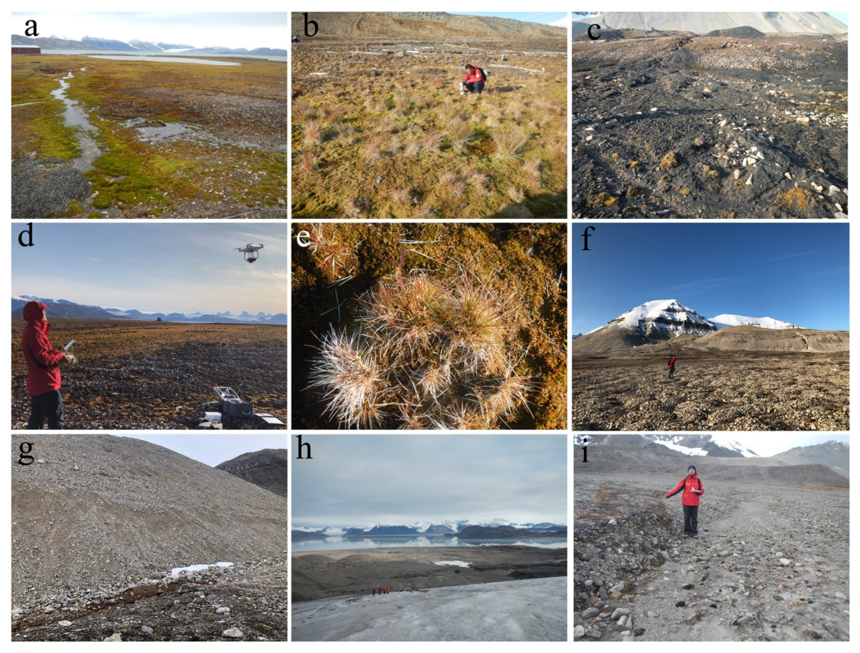
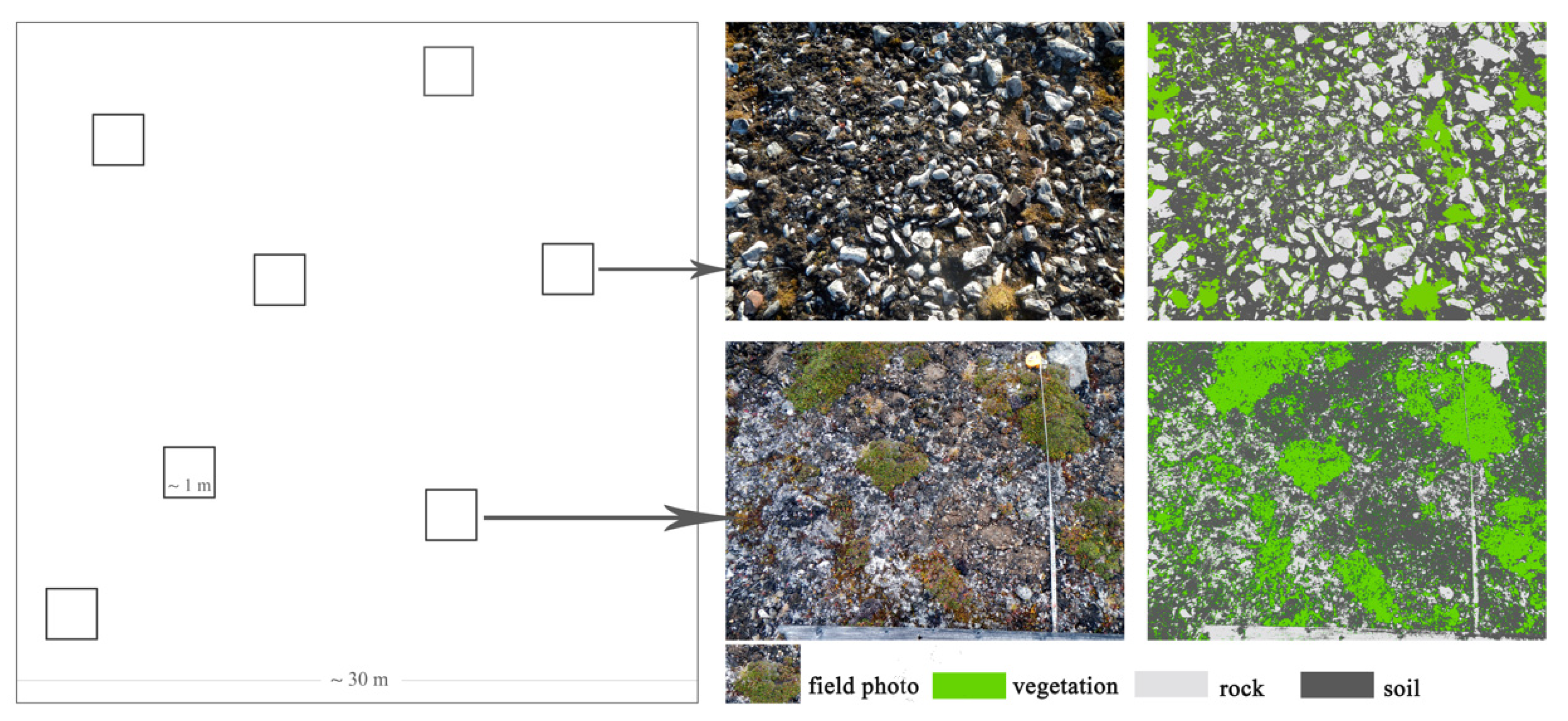
2.3. Field Survey Data

On-site surveys of vegetation and glaciers in the coastal zone around Ny-Ålesund were conducted on 12–29 August 2019. The locations of the survey plots are shown in Figure 1, and photographs of the surveys are shown in Figure 2. The surveys were carried out to obtain the location and photographs of vegetation, glaciers and other land cover in the study area as ground truth samples for the remote sensing image classification. The vegetation cover and vegetation types in the observation plots were assessed and recorded. The on-site assessment method for vegetation coverage is shown in Section 3.1. The locations of all on-site survey plots were recorded by a handheld GPS.

2.4. Temperature and Precipitation Data

Temperature and precipitation are important environmental elements that influence the distribution and changes of vegetation and glaciers in the Arctic. The temperature and precipitation data for Ny-Ålesund from 1984 to 2020 were downloaded from https://seklima.met.no/observations/ (accessed on 18 March 2021), a website that was established by the Norwegian Meteorological Institute. The meteorological observation station was located in the center of Ny-Ålesund at 78.9243°N and 11.9312°E, approximately 8 m above mean sea level (station id SN99910). The temperature and precipitation observation data from 1984 to 2020 are shown in Figure 3.

3. Methods

3.1. Remote Sensing Analysis of Vegetation Coverage

The vegetation coverage rate (VCR), which refers to the percentage of the total plot area that is covered by vegetation, is an important indicator to describe vegetation growth and changes. The vegetation coverage data obtained from field surveys and a remote sensing inversion model of vegetation coverage based on NDVI (the normalized difference vegetation index) were used to analyze the change in the vegetation coverage in the study area over a time series. Where there is no, or inadequate, on-site vegetation coverage survey data, the FVC (fractional vegetation coverage) model was generally used to evaluate vegetation coverage [25,26,27,28]. The FVC formula is as follows:
FVC = ( NDVI p i x e l NDVI 0 ) / ( NDVI NDVI 0 ) ,
where NDVI p i x e l is the NDVI of a certain pixel, NDVI 0 is the NDVI value of bare land without any vegetation coverage, and NDVI is the pixel with the largest NDVI value in the study area. According to the field survey (Figure 2b), in the study area, NDVI represented a pixel with a vegetation coverage of almost 100%, and NDVI 0 was calculated by the average NDVI value of the pixels belonging to dirt roads, the town square and the airport runway in Ny-Ålesund. For example, the NDVI and NDVI 0 , taken from the Landsat image of 1985 in the study area were 0.6899 and 0.0659, respectively.
For terrestrial vegetation in high latitude areas where the vegetation coverage is generally less than 60%, there is a linear correlation between the NDVI value and the vegetation coverage. The vegetation coverage calculated by the FVC model is also linearly related to the true ground vegetation coverage [28,29]. Because the spatial resolution of the commonly used Landsat remote sensing images is 30 m, the surveyed vegetation coverage samples obtained on site were adapted to the spatial scale of the image pixels. Therefore, we used at least five quadrats (1 m × 1 m) randomly selected within a 30 m × 30 m plot. A series of processes were conducted to estimate the true vegetation coverage within the plot. These included taking an orthophoto from a camera at 1.5 m height from the ground (which reflected a photographic coverage of approximately 1 m × 1 m), then estimating the vegetation coverage in the quadrat area and finally calculating the average value of all quadrat areas of vegetation coverage within the 30 m × 30 m plot to give the true vegetation coverage. The evaluation method is shown in Figure 4.
Figure 5 shows the unary linear statistical comparison of the true vegetation coverage in the field samples and the FVC estimated value of the remote sensing image at the same location. In general, the FVC image estimation result had a good statistical correlation with the true value (R2 = 0.789). However, the FVC model tended to underestimate the true vegetation coverage. This may be caused by the low solar altitude in the Arctic region or the lack of atmospheric correction methods suitable for remote sensing images in the Arctic region.

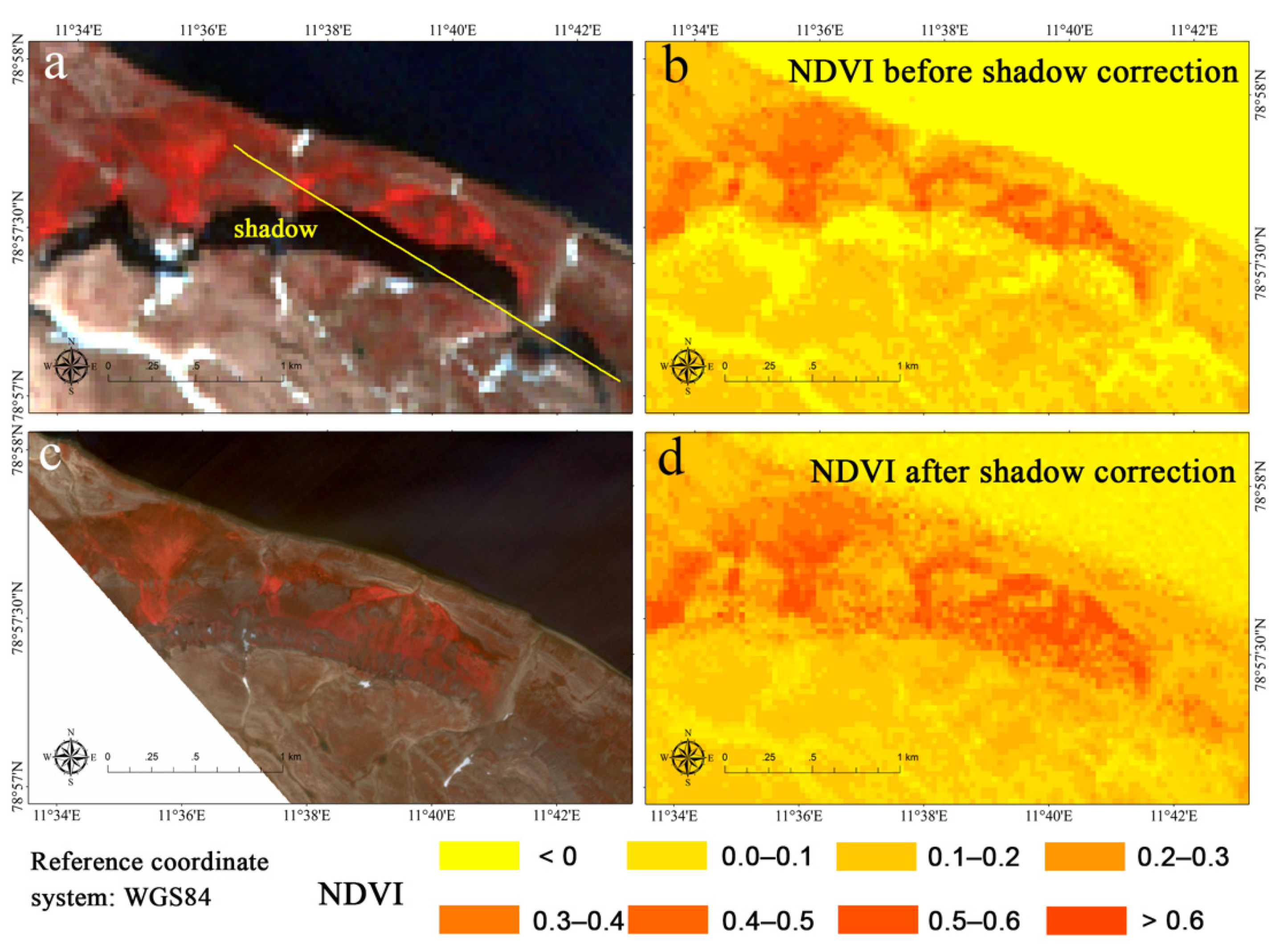
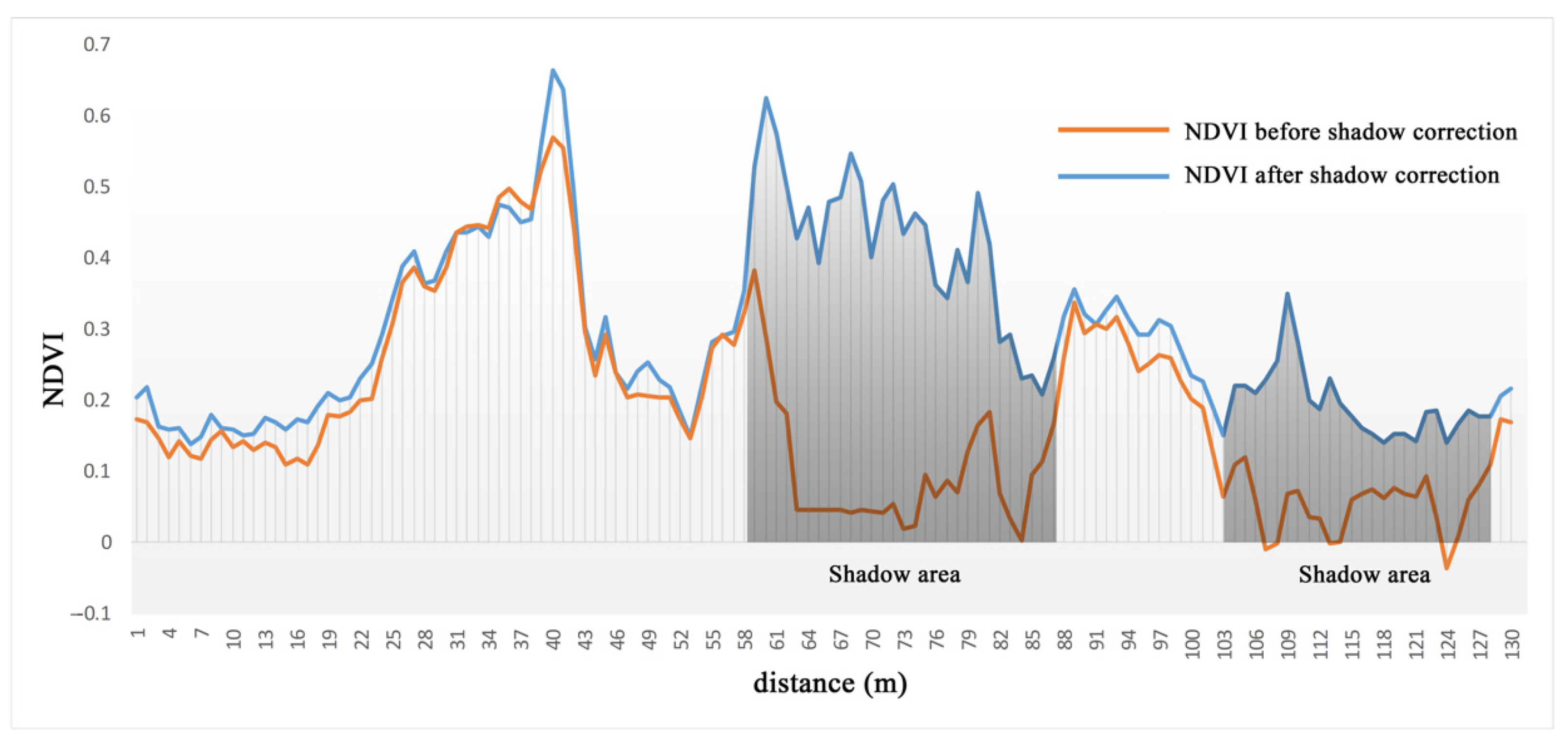
3.2. Removal of Shadows Caused by Low Solar Altitude

The low altitude of the sun in the Arctic is one of the main problems for remote sensing monitoring in this region. The steep-area shadows caused by the low solar elevation angle are an important issue for remote sensing monitoring of vegetation and glaciers in polar regions, especially on mountainous coasts with substantial topographic relief [2]. Jiang et al. [30] indicated that the shadow does influence the estimation accuracy of vegetation features, for example, the NDVI value shows obvious nonlinear characteristics.
To solve this problem, the normalized dark pixel index (NDPI) was applied in the current study. The NDPI, which was first used by [31,32] for reducing the influence of cloud shadow and mountain shadow on vegetation classification in remote sensing images, is extremely sensitive to the shadow area in an image and has little correlation with vegetation information. According to the studies of [31,32], the smallest and largest difference in vegetation radiance between the shaded area and the control illuminated area appear in the blue band (400–500 nm) and the SWIR band (2000–2400 nm), respectively. At the same time, the information on vegetation in these two bands is relatively small. Therefore, the NDPI model is defined as follows:
NDPI = ( ρ b l u e ρ s w i r 2 ) / ( ρ b l u e + ρ s w i r 2 ) ,  
where ρ b l u e and ρ s w i r 2 are the reflectance of the atmospherically corrected image in the blue band (for Landsat 8: 450–520 nm) and short-wave infrared band (for Landsat 8: 2038–2356 nm), respectively.
On the basis of statistical analysis of the vegetation pixels in the shadow location and the directly illuminated area in the image, the NDVI of vegetation influenced by shadow was corrected in the current study. The process for deriving the related formula can be found in [33]. The NDVI correction model for the shaded area is as follows:
NDVI c o r r e c t = NDVI o r i g i n a l + k · ( NDPI o r i g i n a l NDPI ( m i n ,   NDVI m a x ) ) ,  
where NDVI c o r r e c t is the NDVI after shadow correction, NDVI o r i g i n a l is the NDVI affected by the shadow, NDPI o r i g i n a l is the calculated value of the normalized dark pixel index of the remote sensing image, NDPI ( m i n ,   NDVI m a x ) is the NDPI of the pixel corresponding to the largest vegetation index among the vegetation pixels of the image. k is the adjustment parameter, which is obtained by calculating the statistical slope of the NDVI−NDPI pixel value. In the shadow correction of the 1985 image, the adjustment parameter k has a value of −0.386, and moreover the shadow correction adjustment parameters were estimated on an image-by-image basis.
Figure 6b shows the uncorrected NDVI of the shadow area in the Landsat 8 OLI image (Figure 1a) acquired on 1 August 2015. Figure 6d shows the NDVI after shadow correction. It can be seen from Figure 6d that the NDVI of the pixels in the shadow area was effectively restored. Figure 7 shows the NDVI on the transect (yellow line) within Figure 6a, which clearly demonstrates the effect of shadow removal. The Gaofen-2 satellite remote sensing image (Figure 6c) acquired on 28 August 2015, did not produce shadows in the area shown in Figure 6a because of the difference in the azimuth of the sun at the time of acquisition.

3.3. SVM Classification

A lack of training samples is a basic problem in the classification of remote sensing images covering coastal wetlands, especially for Arctic areas, and field investigations are difficult to conduct. To solve this problem, the SVM (support vector machine) classification method based on statistical learning theory [34] was applied in this study. The advantages and characteristics of SVM are that it can effectively solve the problem of small samples in image classification and solve the issue of linear indivisibility caused by high dimensional features through the kernel method. SVM is one of the most widely used techniques in land cover classification [35,36]. In the SVM classification process, ENVI 5.3 software was used. Taking the Landsat image classification as an example, the radial basis function was chosen as the kernel, the value of the gamma parameter used in the kernel function was set to 0.167, and the penalty parameter was specified as 100. The vegetation, glaciers and other land cover types were classified using the data from the survey sites (Figure 1) and expert interpretation as the training samples (70% of all samples) and validation samples (30% of all samples). The overall classification accuracy of all the Landsat images was over 90% with all the kappa parameters larger than 0.87. A human–computer interactive post-classification process was carried out to correct the misclassified cover types, regions and pixels.

4. Results and Analysis

4.1. Spatial and Temporal Changes in Vegetation

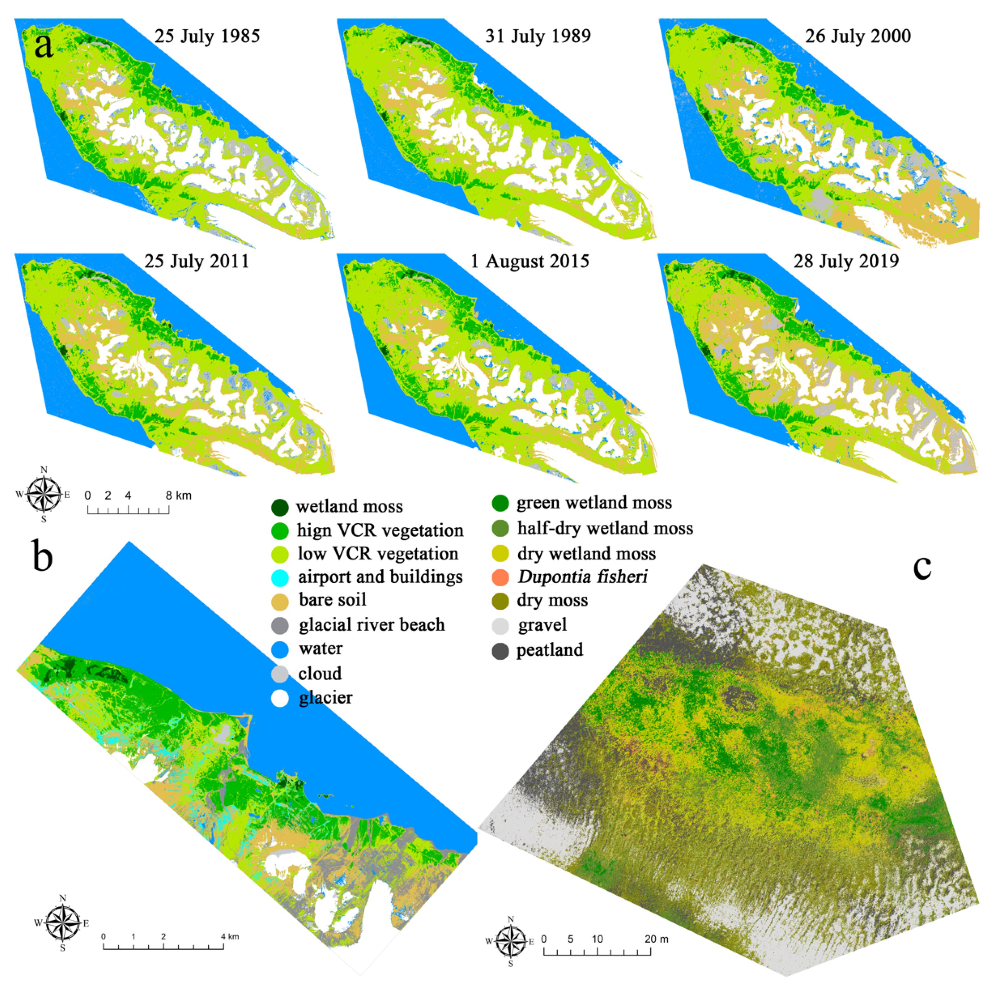
4.1.1. Multi-Resolution Monitoring Results for Vegetation

To examine the ability of remote sensing to identify different types of vegetation and other landcover types in the study area, Landsat series satellite data with a spatial resolution of 30 m, Gaofen-2 satellite data with a spatial resolution of 4 m, and UAV multispectral remote sensing data with a spatial resolution of 3 cm, combined with site survey data, were used to establish different classification systems. The classification results using SVM are shown in Figure 8. The results demonstrated that although the spatial resolution of Gaofen-2 was higher than the Landsat satellite images, Gaofen-2 could not further distinguish different vegetation types. The reason was that all the pixels had mixed vegetation types (Figure 2b,c,e), except for wetland moss (Figure 2a), at the spatial scale of the two image types (30 m and 4 m). Gaofen-2 data were able to further classify landcover types such as the airport and buildings.
The UAV multi-spectral remote sensing images with a spatial resolution of 3 cm could distinguish different types of plants in fine detail. The classification results are shown in Figure 8c. The spatial distribution of individual species and plants in the polar tundra was separable at a centimeter-level (Figure 2). The UAV images accurately identified tundra grasses in the surveyed area. They also enabled further subdivision of moss into wetland and dryland moss, as well as into growing or dormant moss. Peatland, gravel and bare land could also be clearly distinguished.

4.1.2. Monitoring of Temporal and Spatial Changes in Vegetation Distribution

The selected satellite remote sensing images were acquired at the end of July and the beginning of August (summer), and therefore no vegetation was covered by snow in the study area. The topography of the study area was characterized by a high central spine of mountains and low coastal zones around the spine. The glaciers were mainly distributed in the middle of the peninsula, whereas vegetation was mainly distributed near the coast. The distribution of wetland moss communities was relatively concentrated, mainly in the north and southwest of the peninsula (Figure 8). Areas with steeper and flatter terrain were the main distribution areas of tundra vegetation with a low coverage rate. Here, the high coverage rate was classed as more than 30%, the low coverage rate was 5–30%, and areas with coverage rate less than 5% were treated as bare land in the classification results.
The change of vegetation in the Arctic is an extremely sensitive indicator of global warming and human activities [37,38]. During the 35 years from 1985 to 2019, the area of vegetation distribution with a high coverage rate in the study area showed an upward trend (Figure 9a). Notably, the low coverage rate area and the total vegetation area of the monitoring area in 2000 were underestimated because, when the Landsat 7 image was acquired in 2000, the low vegetation coverage area was partly covered by cloud. The monitoring results of the low coverage tundra plants in 2019 were also too small because, when the Landsat 8 image was captured on 28 July 2019, the solar altitude angle was very low (Table 1), which reduced the detectability of plant targets.
The wetland moss area with high water requirements increased (Figure 9b), which may be caused by the accelerated melting of glaciers. Glacial meltwater has continuously increased the high-water content area in the moss communities of the lower wetlands, which can easily store water.

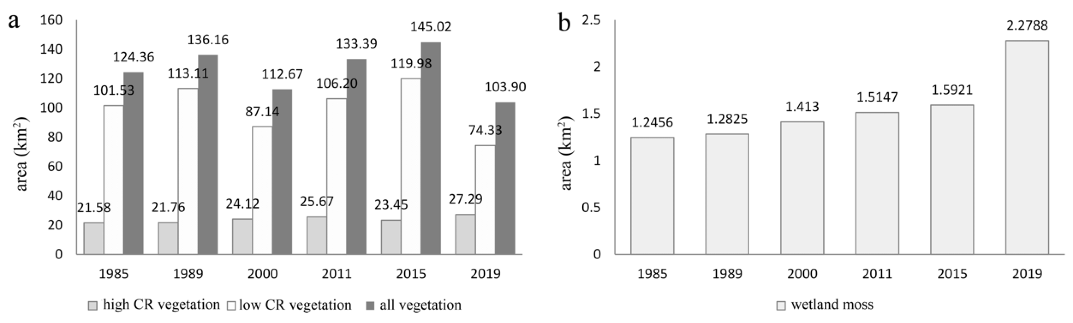
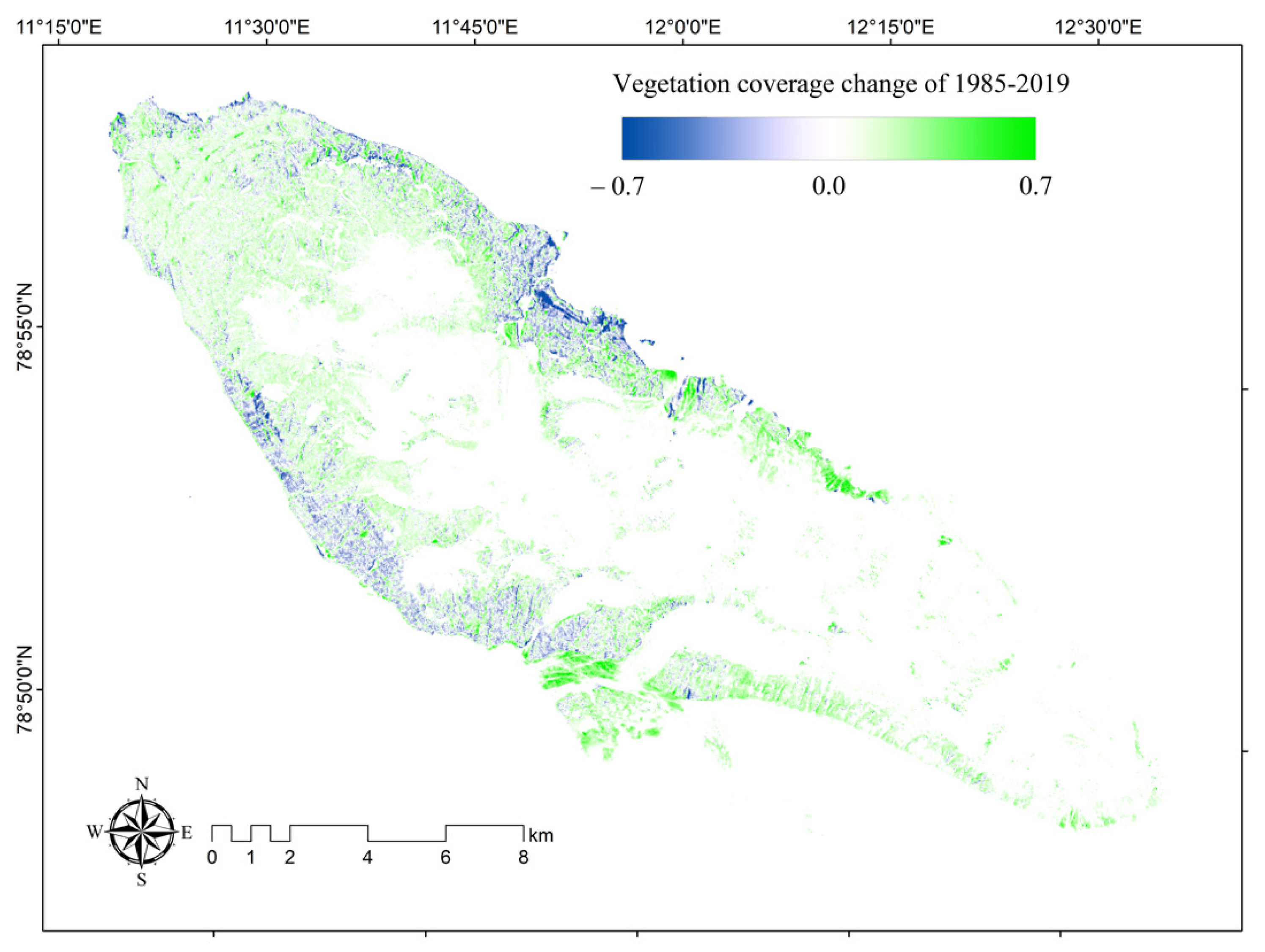
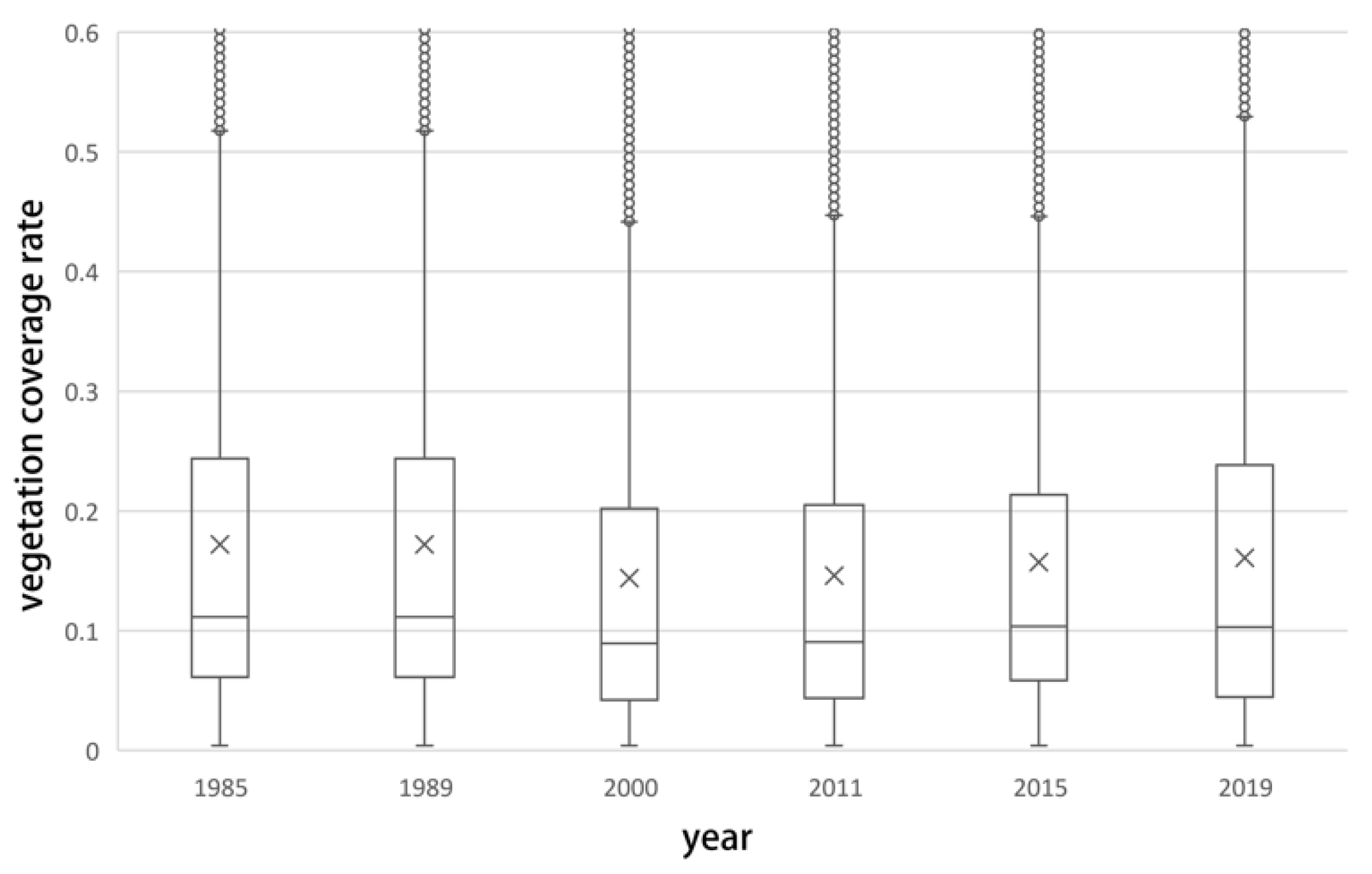
4.1.3. Monitoring the Temporal and Spatial Changes in Vegetation Coverage

Figure 10 shows the spatial changes in vegetation coverage from 1985 to 2019, which were derived from the FVC estimation results. First, the area with the most obvious increase in coverage was on the beach in the lower reaches of the glacier meltwater valley [24]. This was due to the gradual decrease in the glacier meltwater, which meant that the original wide beach no longer had water flowing over it throughout the summer. Especially after 2000, a large quantity of vegetation gradually developed in this location (Figure 2i). The unique water and nutrient supply conditions and geographical advantages allowed this wetland vegetation to grow rapidly. Second, the original wetland moss distribution area and coverage did not change. This showed that these areas could still obtain an abundant water supply. There was an increase in the wetland moss distribution area with high coverage. Third, the vegetation coverage of Ny-Ålesund and the areas surrounding the airport, where human activities were frequent, decreased significantly. Fourth, vegetation coverage in high-altitude areas increased, while vegetation coverage at low altitudes and on steep slopes declined.
To analyze temporal change, a box plot of vegetation coverage in six different phases during the study period was created using pixels (30 m × 30 m) as the unit. As mentioned before, owing to cloud occlusion and the low solar altitude, the information extracted for low coverage areas in 2000 and 2019 was underestimated. The box plot overcomes the problem of inaccurate monitoring of vegetation distribution caused by cloud cover and low solar altitude angle to some extent. Vegetation coverage had a trend of first decreasing and then increasing, with the year 2000 as the breaking point (Figure 11). The median, mean and quartile values for vegetation coverage all show similar trends. After 2000, the coverage of the majority of pixels (represented by the box) increased. The average value in all years was greater than the median value, which indicated that the number of pixels with low vegetation coverage was still dominant [24].

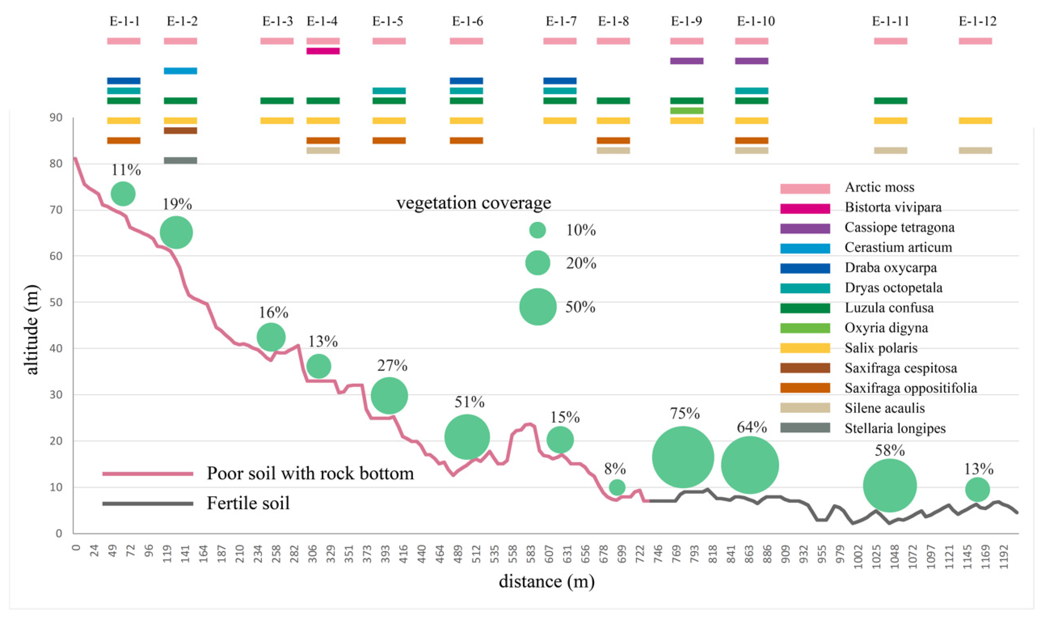
4.1.4. The Relationship between Vegetation Distribution, Change and Elevation

Altitude is an important factor in determining the distribution of vegetation in coastal zones with glaciers [9]. As the elevation increases, especially at higher altitudes, some areas are covered by perennial glaciers and vegetation cannot grow. Furthermore, the barren and bare fragmented rocks in high-altitude areas are not suitable for the survival of vegetation owing to weathering, especially erosion by ice and snow [16]. In addition, the slope of most areas increases with an increase in altitude and the barren soil does not conserve water, making it difficult for vegetation to survive (Figure 2g).
The field work section E-1 (Figure 1) was used as an example to analyze the relationship between the distribution of different types of arctic vegetation, vegetation coverage and altitude. As shown in Figure 12, there were two distinct types of sediments. One was an area with ice and snow eroded rock fragments as the bottom material at a higher elevation and the other was a more fertile region with soil-based bottom material in a low-altitude area near the coast (Figure 2). In general, the vegetation coverage in the rocky bottom area increased with a decrease in altitude. However, the vegetation coverage in the fertile soil substrate area showed a decreasing trend in the seaward direction, and the largest vegetation coverage appeared at the junction of the rocky basement and the fertile soil basement.
In terms of vegetation type distribution, Arctic moss and Salix polaris grew at different altitudes and on different sediment types [39]. Stellaria longipes and Cerastium articum only appeared in high altitude areas, while Cassiope tetragona only appeared in low altitude areas. Only four types of vegetation existed within approximately 200 m of the coast: Arctic moss, Silene acaulis, Lusula confusa and Salix polaris. Most of the site survey plots had more than five types of vegetation, even when the plot’s vegetation coverage averaged only 13%, which showed that the study area was relatively highly biodiverse.
The statistical relationship between all vegetation coverage pixels (vegetation FVC assessment coverage greater than 5%) and their elevation in the study area is shown in Figure 13. First, the highest vegetation growth was approximately 678 m. Notably, the highest position of vegetation growth tended to decrease after the year 2000. Second, the vegetation coverage in 2019 increased at different altitudes. We found that 95% of the pixels with a coverage rate of 30% or more were located in areas less than 50 m above sea level [17], and 85% of the vegetated pixels with an altitude of more than 200 m had vegetation coverage below 20%.
Figure 14 shows the changes in the coverage of vegetation pixels at different slope angles over the past 35 years. In general, vegetated pixels on steep slopes tended to decrease in vegetation coverage (the densely contoured areas correspond to steep slopes in Figure 19), whereas vegetation coverage on shallow slopes tended to increase. The coverage of most vegetation pixels with increased coverage was still below 30%.

4.2. Spatial and Temporal Changes of Glaciers

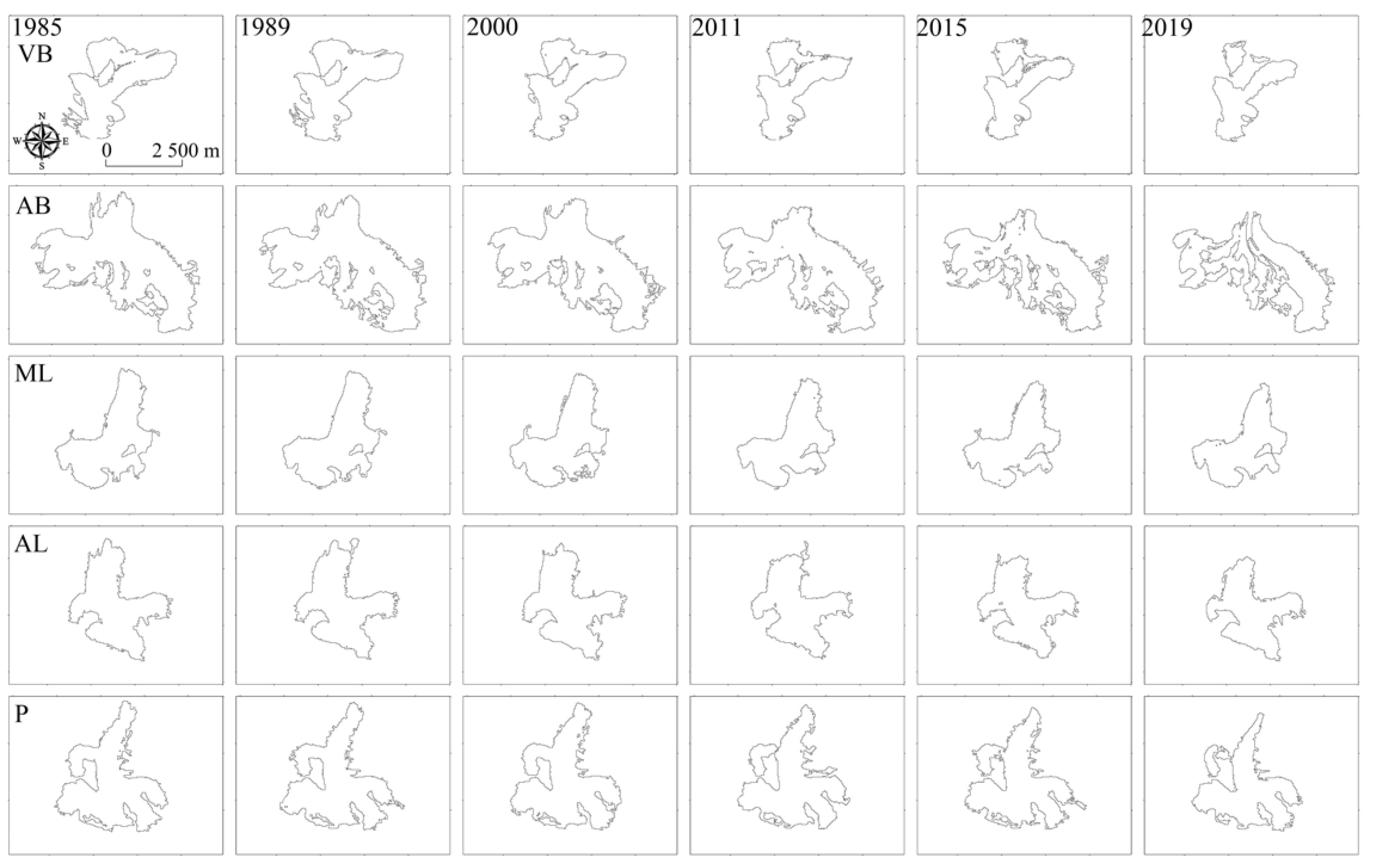
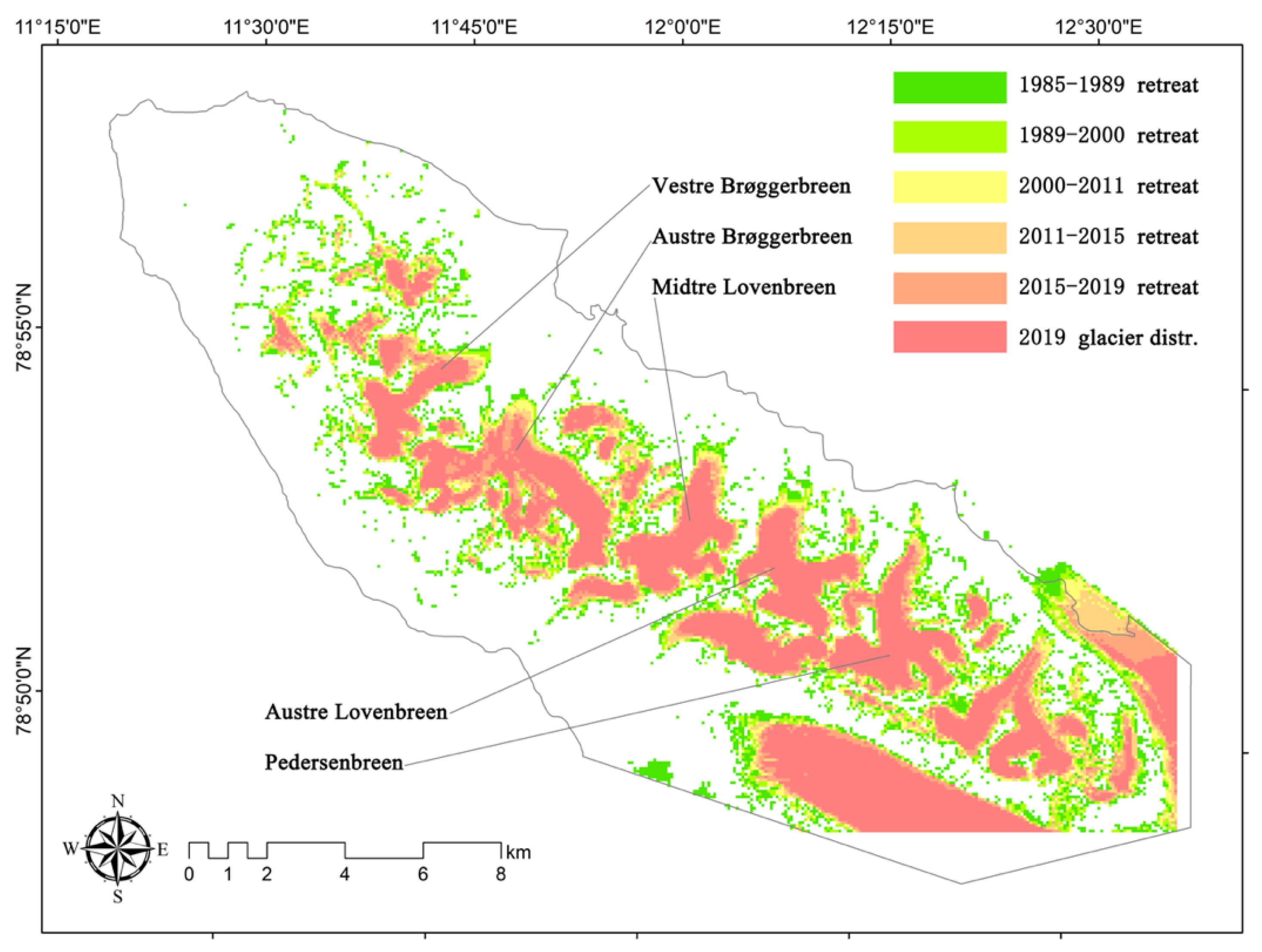
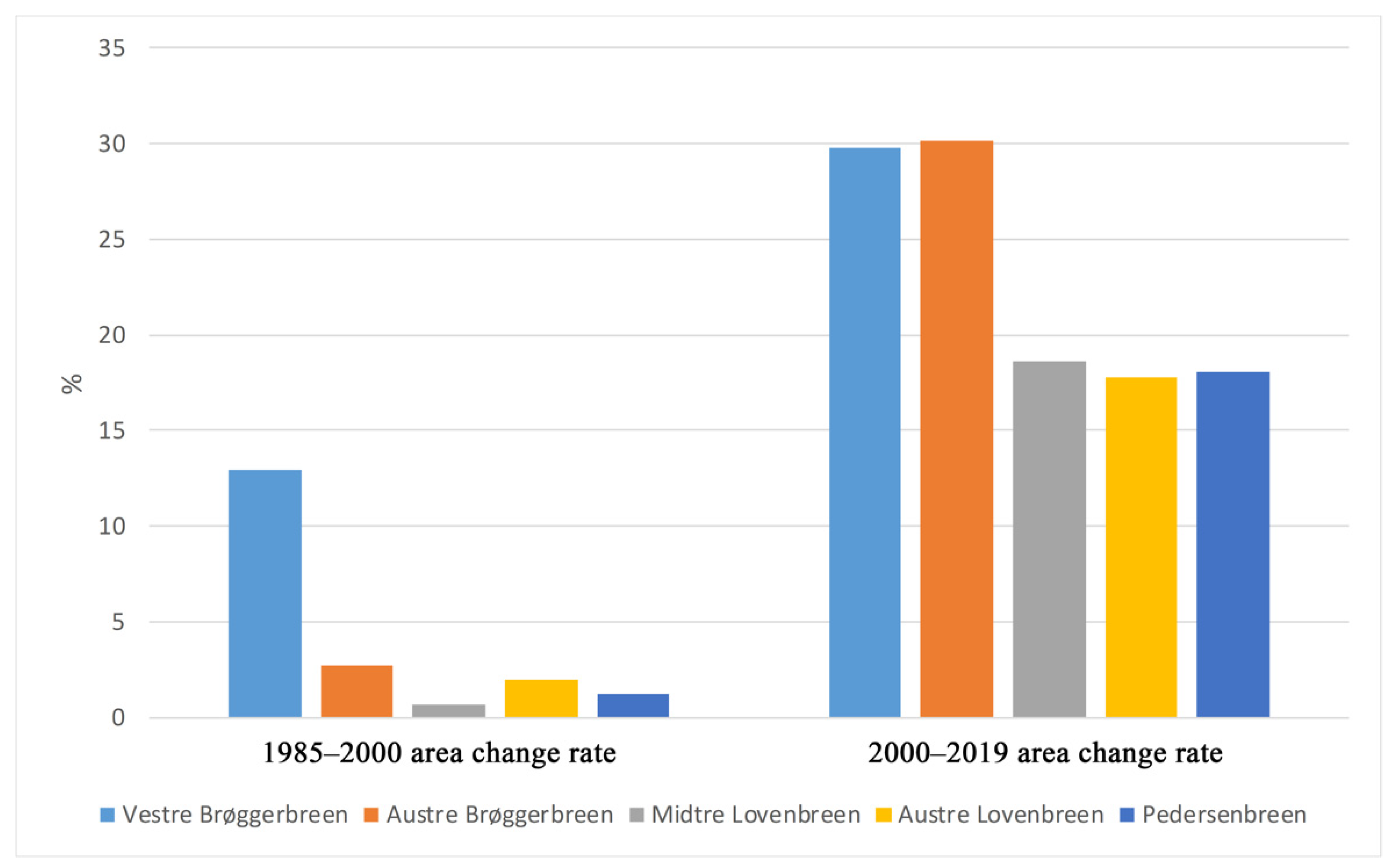
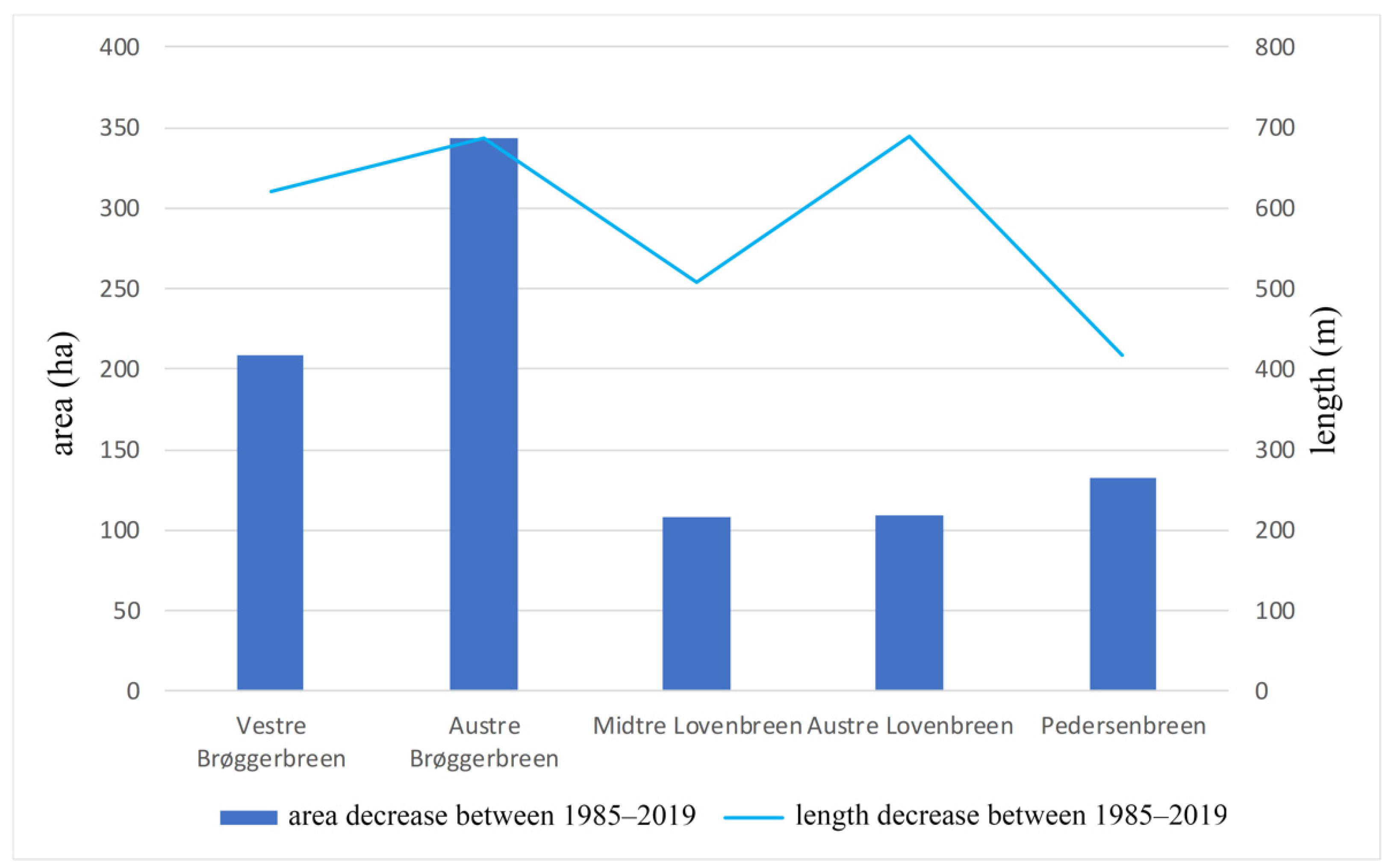
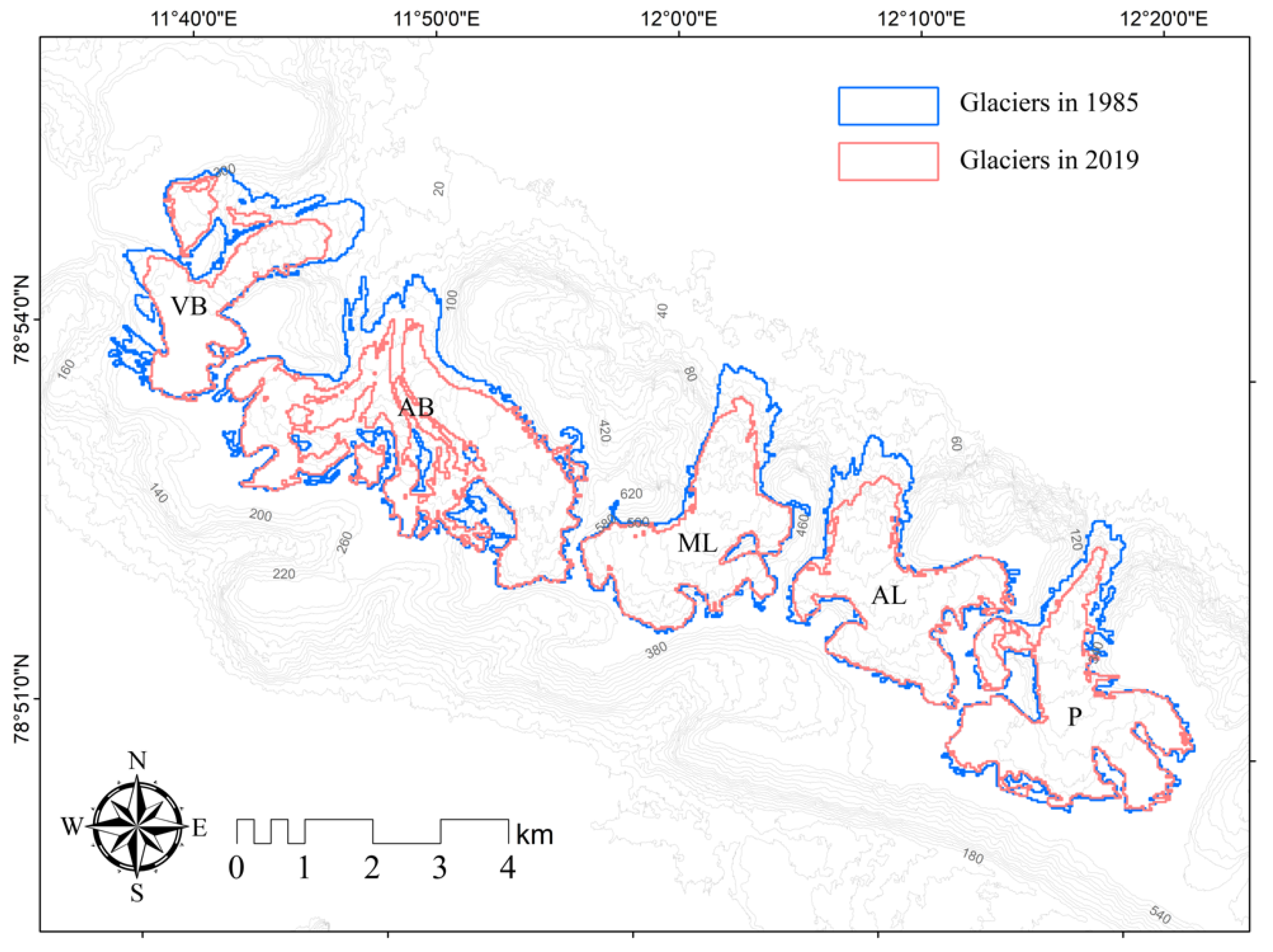
4.2.1. Remote Sensing Monitoring of Temporal and Spatial Changes of Glaciers

The satellite images used in this study were all acquired in July and August when there was minimal seasonal snow cover in the study area. The results of the SVM method used to classify and extract glacier information in different years are shown in Figure 15. It was found that the five major glaciers had similar but varying rates of retreat. The main characteristic was that, in the plane projection, the length of the glaciers became shorter, the width became narrower, and the bits of the glacier broke off, for example, the Vestre Brøggerbreen (VB), Austre Brøggerbreen (AB) and Pedersenbreen (P) glaciers (Figure 15). At the same time, according to the spatial analysis of glacier degradation in Figure 16, some small, scattered glaciers that existed in 1985 had disappeared completely by 2019, although these could have been ice and snow patches that were not completely melted because of low temperatures. Glaciers became more concentrated in the center of the study area image. According to the DEM analysis, the glaciers were increasingly distributed in high altitude areas.
A bar plot of the change rates for five selected glaciers before and after 2000 is shown in Figure 17. In the 15 years before 2000, the plane projection area of four of these glaciers (all except the VB glacier) decreased by a small extent, all below 3%. In the 20 years since 2000, all glaciers have experienced accelerated retreat [40]. The area reduction rate of the Midtre Lovenbreen (ML), Austre Lovenbreen (AL) and P glaciers was more than 15%, while the reduction rate of the VB and AB glaciers reached nearly 30%. In total, approximately 82% of the melted glacier area retreated after 2000. The VB and AB glaciers were closer to the mouth of the bay than the other three glaciers (Figure 1 and Figure 16); their area and length reduction were the largest (Figure 18) [7,41]. The length of the glacier here is the length of the line of maximum slope along the direction of the slope gradient from the highest elevation to the lowest.

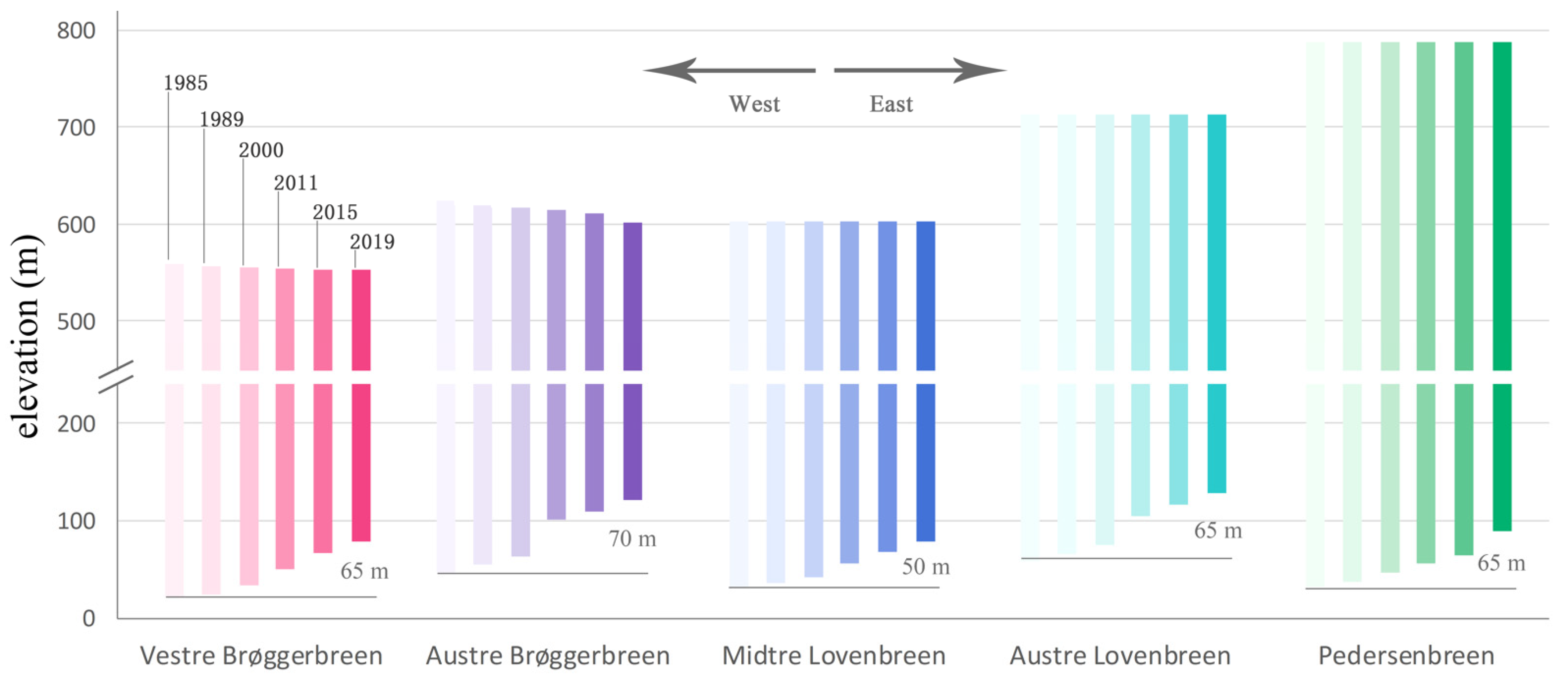
4.2.2. The Relationship between Glacier Distribution, Change and Elevation

All the glaciers were distributed on the north side of Brøggerhalvøya mountain (Figure 19). The contours of the glacier surface were evenly distributed, with a relatively steep slope only at the lower edge of the glaciers. During the monitoring period, the glaciers all retreated [42]. The elevation of the lower edge of the glaciers became higher, and the upper part of the glaciers also tended to move to lower altitudes (that is, to the north), although the overall distance of movement was small.
Figure 20 shows the change in height of the five glaciers in the study area between 1985 and 2019. The curve in the lower part of the figure is a cross section of each glacier along its gradient direction. The elevation of the lowest part of the five glaciers increased by 50–70 m during the 35-year study period.

5. Discussion

5.1. Analysis of Temperature and Precipitation on Vegetation and Glaciers

The annual average temperature, annual maximum temperature, and annual precipitation generally showed different trends over time with 2000 as the breaking point. The temperature from 1985 to 2000 was generally stable, except for the lowest average annual temperature that occurred in 1988. The overall maximum temperature showed a downward trend, with the exception of the extremely high temperatures in 1997 and 1998 [43]. From 1985 to 2000, precipitation generally showed a slight downward trend and, from 2000 to 2019, it showed a clear upward trend (Figure 3).
To a certain extent, these patterns explain why the vegetation coverage in high-altitude areas and on steep slopes declined prior to 2000. There is little replenishment of water sources from runoff at high altitudes, and it is difficult to conserve water in areas with steep slopes. At the same time, the stable temperature did not contribute to an increase in vegetation coverage. However, after 2000, the trends in both temperature and precipitation were beneficial for vegetation growth and led to an increase in vegetation coverage.
On the basis of the monitoring results in Section 4.2, the reduction in glacier area was not obvious before 2000. A reduction in glacier area can be caused by insufficient precipitation and higher temperatures [24]. After 2000, although precipitation increased to a certain extent, the overall quantity was still relatively low, and the annual average temperature increased significantly, which intensified glacial retreat.
Whether before or after 2000, accelerating glacial meltwater moistened the alluvial plains near the coastline. As a result, the distribution area of wetland moss is gradually increasing. Especially after 2000, the obvious increase in precipitation further promoted the prosperity of wetland moss. The retreat of glaciers leaves more space for the growth of vegetation; and at the same time, the reduction in glacier coverage means that fewer hillside areas are supplemented by glacier melt water, leading to a decline in the vegetation coverage.
In the future, it can be expected that, as the temperature in the study area continues to rise, the area of glaciers will undoubtedly continue to decrease. The reduced glaciers will leave more space for vegetation growth at low altitudes [24,44], but the vegetation coverage at high altitudes and on steep slopes will increase very slowly [38]. In addition, as the amount of glacier meltwater continues to decrease, the runoff width of the stream formed by the meltwater will eventually decrease, more river valley land will grow vegetation and the distribution of high coverage vegetation will increase [9].

5.2. The Spatial and Temporal Resolution of Images in Arctic Area Monitoring

Long periods of ice and snow cover and short vegetation growth times are the most significant climatic characteristics in the Arctic region [1,45]. Against the background of global warming in recent years, the Arctic summer ice and snow cover is gradually becoming shorter [11,46,47], but the time for vegetation growth is still only 2–4 months [2]. In the Arctic region in the current study, vegetation growth occurs from July to September, while the best time for monitoring vegetation with remote sensing is from the end of July to the beginning of August, because in this period vegetation growth is at its highest [48] and the daily mean temperature is above zero. Therefore, from the archived Landsat series image data set, cloud free images with a data acquisition time between July 25 and August 5 were selected. The daily mean temperatures of these days were the hottest in all study years (https://seklima.met.no/observations/ (accessed on 18 March 2021)). Owing to the serious problem of cloud and fog in the Arctic summer, only the remote sensing images in 1985, 1989, 2000, 2011, 2015 and 2019 met the study criteria. Considering that, in the Arctic region, the vegetation growth cycle is short and that the vegetation growth state can change substantially in a very short time, this strict data selection method can ensure the comparability of vegetation information obtained in different years. At the same time, the large difference in the solar altitude angle of the images taken at a large time interval should be considered because this will introduce more uncertainty to the monitoring of Arctic vegetation and glaciers. Where human development activities have little impact, the changes in Arctic vegetation and glaciers are relatively slow. Therefore, a time interval of 5–10 years to study the changes of vegetation and glaciers in the study area can capture the key change characteristics [24]. When studying the distribution and change characteristics of Arctic vegetation in a phenological cycle, it is difficult to obtain sufficient data only by means of satellite remote sensing because clouds and rainfall occur for most of the Arctic summer, and the limited time of cloud free weather does not often coincide with the satellite acquisition time.
The spatial resolution of remote sensing images is also a key issue to be considered for the monitoring of Arctic vegetation and glaciers. In the early and late stage of vegetation growth, sparse coverage and low chlorophyll content make it difficult to effectively monitor vegetation in medium spatial resolution (such as 30 m/pixel) images, and high spatial resolution images need to be used, such as 4 m resolution Gaofen-2 and 0.5 m resolution WorldView images. In the period of vigorous vegetation growth, when monitoring vegetation at a species level, UAV remote sensing is the only effective means [49] because of the small scale of individual plants growing in the high-latitude Arctic. According to the results in Section 4.1, UAV remote sensing with a spatial resolution of 3 cm can effectively classify vegetation species. Compared with the Landsat data with 30 m spatial resolution, the Gaofen-2 data with 4 m spatial resolution greatly improved the spatial resolution, but it still could not distinguish vegetation species [15,50]. However, high spatial resolution images could better capture the boundary details of land cover types.

5.3. The Influences on Vegetation and Gacier Remote Sensing Monitoring in Arctic Areas

Compared with other regions of the Earth, in the Arctic the solar altitude angle is always low (Table 1), which affects the radiation energy received from the ground targets by the optical sensor on the satellite, resulting in low radiation resolution and a small signal-to-noise ratio of the image [51]. In the study area, the mountain shadow formed by the small incidence angle of the sun further affected the monitoring of ground vegetation and glaciers. In the current paper, an NDPI index that is sensitive to shadow information and insensitive to vegetation information was introduced. By establishing a correction model, the NDVI of vegetation affected by mountain shadow was corrected to some extent. Many studies have shown that when the vegetation coverage is greater than 60%, the evaluation value of NDVI will be saturated [29,52,53]. According to the field survey data and FVC evaluation results, only 1.8% of the vegetation pixels had a vegetation coverage rate greater than 60%, and these areas were mainly located in the wetland moss distribution area. According to the monitoring results of the current paper, the distribution area of wetland moss did not change during the monitoring period. Although the solar altitude angle is low in the Arctic summer, the solar irradiation time is long, and lasts for 24 h a day.
The impact of clouds and fog is a more serious issue in summer during the growth period for Arctic vegetation; it is often impossible to capture cloud-free data for entire summers [54]. This results in a lack of satellite remote sensing images that meet the conditions every year during the best monitoring period [26]. The best methods for monitoring the Arctic region under the influence of clouds and fog are UAVs and field investigations. For UAV monitoring, researchers still need to pay attention to the impact of wind speed on flight safety and platform stability.

5.4. The Role of Topographic Data in Glacier Melting Monitoring

Compared with optical satellite remote sensing images, high-resolution DEM data that can reflect the topographic changes of the Arctic are very scarce. Without the influence of large-scale human development activities, primarily glacier changes can cause topographic fluctuations in the Arctic. The melting and movement of glaciers can be obtained through the analysis of changes in topographic monitoring data at different times. Obviously, the description of glacier change given in Section 4.2 was not comprehensive, and more information is needed on glacier change in the vertical direction.

6. Conclusions

Global climate change has the greatest impact in the Arctic, and the fragile Arctic ecosystems are responsive to even subtle variations in climate. The changes in the ecosystem of the regions affected by climate change are not isolated, and they are closely related to the surrounding environmental conditions and changes in those environmental conditions.
In this study, we monitored and analyzed vegetation coverage and glacier changes in the area surrounding Ny-Ålesund in the Arctic using remote sensing image data with different spatial resolutions and platforms to form a long time series and with the support of field survey data, topographic data and climate change data. The main conclusions are as follows.
The vegetation types in the high-latitude tundra areas of the Arctic are complex, with mixed species of plants, which are individually small in scale. Therefore, although the Gaofen-2 image had a spatial resolution up to 4 m, it still could not provide a more detailed vegetation classification than Landsat images with a spatial resolution of 30 m. The UAV multi-spectral images with a spatial resolution of 3 cm did achieve a detailed classification of vegetation types. In terms of the temporal changes of vegetation, the area of vegetation with high coverage generally increased in the study period, while the average area of vegetation with low coverage, total vegetation and vegetation pixel coverage decreased before 2000 and then increased. In terms of the spatial distribution of vegetation, the areas with the highest vegetation coverage and the most concentrated areas were located in low-altitude flat regions close to the coastline, and on both sides of streams and valleys fed by glacial meltwater.
Remote sensing monitoring and analysis of the temporal and spatial changes of five selected glaciers in the study area were conducted. The overall area and length of the five glaciers have decreased from 1985–2019 by 15–30%, accelerating since 2000. The lowest altitude has increased by approximately 50–70 m over 35 years, and with fragmentation of the glacier snouts.
Climate change is the most important factor affecting vegetation and glacier changes. According to climate observation data, both the temperature and precipitation increased in the study area after 2000, but before 2000 they were relatively stable (precipitation dropped slightly). This explains the different change characteristics of vegetation and glaciers in the time series monitoring results with the year 2000 as the breaking point.

Author Contributions

G.R. conceived and designed the research, processed the data and wrote the manuscript draft. Y.M. and C.C. helped design the research and revise the manuscript. G.R. and J.W. conducted the fieldwork and analyzed the data, Y.L., P.W. and X.L. contributed materials and helped conceive the research and review the manuscript. All authors have read and agreed to the published version of the manuscript.

Funding

This study is jointly supported by the National Key R&D Program of China (2018YFC1407202), the National Natural Science Foundation of China (42076189) and the Dragon-4 project, China under grant 32405.

Institutional Review Board Statement

Not applicable.

Informed Consent Statement

Not applicable.

Acknowledgments

The authors would like to thank the USGS for providing satellite images. We also thank Leonie Seabrook for editing the English text of a draft of this manuscript.

Conflicts of Interest

The authors declare no conflict of interest.

References

  1. Reynolds, J.F.; Tenhunen, J.D. Ecosystem response, resistance, resilience, and recovery in Arctic landscapes: Introduction. In Landscape Function and Disturbance in Arctic Tundra, Ecological Studies; Reynolds, J.F., Tenhunen, J., Eds.; Springer: Heidelberg, Germany, 1996; Volume 120, pp. 3–18. [Google Scholar]
  2. Stow, D.A.; Hope, A.; McGuire, D.; Verbyla, D.; Gamon, J.; Huemmrich, F.; Houston, S.; Racine, C.; Sturm, M.; Tape, K. Remote sensing of vegetation and land-cover change in Arctic Tundra Ecosystems. Remote Sens. Environ. 2004, 89, 281–308. [Google Scholar] [CrossRef] [Green Version]
  3. Intergovernmental Panel on Climate Change. Climate Change 2013: The Physical Science Basis; Working Group II Contribution to the IPCC 5th Assessment Report; Cambridge University Press: Cambridge, UK, 2013. [Google Scholar]
  4. Polyak, L.; Alley, R.B.; Andrews, J.T.; Brigham-Grette, J.; Cronin, T.M.; Darby, D.A.; Dyke, A.S.; Fitzpatrick, J.J.; Funder, S.; Holland, M.; et al. History of sea ice in the Arctic. Quat. Sci. Rev. 2010, 29, 1757–1778. [Google Scholar] [CrossRef]
  5. Kern, S.; Saleschke, L.; Spreen, G. Climatology of the Nordic (Irminger, Greenland, Barents, Kara and White/Pechora) Seas ice cover ased on 85 GHz satellite microwave radiometry 1992–2008. Tellus Ser. A—Dyn. Meteorol. Oceanogr. 2010, 62, 411–434. [Google Scholar] [CrossRef]
  6. White, J.W.C.; Alley, R.B.; Brigham-Grette, J.; Fitzpatrick, J.J.; Jennings, A.E.; Johnsen, S.J.; Miller, G.H.; Nerem, R.S.; Polyak, L. Past rates of climate change in the Arctic. Quat. Sci. Rev. 2010, 29, 1716–1727. [Google Scholar] [CrossRef]
  7. Laffly, D.; Mercier, D. Global change and paraglacial morphodynamic modification in Svalbard. Int. J. Remote Sens. 2002, 23, 4743–4760. [Google Scholar] [CrossRef]
  8. Anisimov, O.A.; Vaughan, D.G.; Callaghan, T.V.; Furgal, D.; Marchant, H.; Prowse, T.D.; Vilhja lmsson, H.; Walsh, J.E. Climate Change 2007: Impacts, Adaptation and Vulnerability. Contribution of Working Group II to the Fourth Assessment Report of the Intergovernmental Panel on Climate Change. In Polar Regions (Arctic and Antarctic); Parry, M.L., Canziani, O.F., Palutikof, J.P., van der Linden, P.J., Hanson, C.E., Eds.; Cambridge University Press: Cambridge, UK, 2007; pp. 653–685. [Google Scholar]
  9. Yoshitake, S.; Uchida, M.; Ohtsuka, T. Vegetation development and carbon storage on a glacier foreland in the High Arctic, Ny-Ålesund, Svalbard. Polar Sci. 2011, 5, 391–397. [Google Scholar] [CrossRef] [Green Version]
  10. Oechel, W.C.; Vourlitis, G.L. The effects of climatic change on land atmosphere feedbacks in arctic tundra regions. Trends Ecol. 1994, 9, 324–329. [Google Scholar] [CrossRef]
  11. Williams, M.; Eugster, W.; Rastetter, E.B.; McFadden, J.P.; Chapin III, S.F. The controls on net ecosystem productivity along an Arctic transect: A model comparison with flux measurements. Glob. Chang. Biol. 2000, 6 (Suppl. 1), 116–126. [Google Scholar] [CrossRef]
  12. Wadham, J.L.; Tranter, M.; Dowdeswell, J.A. Hydrochemistry of meltwaters draining a polythermal-based, high-Arctic glacier, south Svalbard: II. Winter and early Spring. Hydrol. Process. 2015, 14, 1767–1786. [Google Scholar] [CrossRef]
  13. Pfüller, A.; Ritter, C.; Stock, M.; Shiobara, M.; Lampert, A.; Maturilli, M.; Orgis, T.; Neuber, R.; Herber, A. Ground-based lidar measurements from Ny-Ålesund during ASTAR 2007. Atmos. Chem. Phys. 2009, 9, 9059–9081. [Google Scholar] [CrossRef] [Green Version]
  14. Hisdal, V. Geography of Svalbard, 2nd ed.; Norsk Polarinstitutt (Polarhandbok 2): Oslo, Norway, 1985. [Google Scholar]
  15. Brossard, T.; Joly, D. Probability models, remote sensing and field observation: Test for mapping some plant distributions in the Kongsfjord area, Svalbard. Polar Res. 1994, 13, 153–161. [Google Scholar] [CrossRef]
  16. Brattbakk, I. Flora og vegetasjon. In Svalbardreinen og Dens Livsgrunnlag; Oritsland, A., Ed.; Universitetsforlaget: Oslo, Norway, 1986; pp. 15–34. [Google Scholar]
  17. Spjelkavik, S. A satellite-based map compared to a traditional vegetation map of Arctic vegetation in the Ny-lesund area, Svalbard. Polar Rec. 1995, 31, 257–269. [Google Scholar] [CrossRef]
  18. Engeset, R.V.; Weydahl, D.J. Analysis of glaciers and geomorphology on Svalbard using multitemporal ERS-1 SAR images. Geosci. Remote. Sens. IEEE Trans. 1998, 36, 1879–1887. [Google Scholar]
  19. Winther, J.G.; Oddbjørn, B.; Sand, K.; Gerland, S.; Marechal, D.; Ivanov, B.; Gøowacki, P.; König, M. Snow research in Svalbard–An overview. Polar Res. 2003, 22, 125–144. [Google Scholar]
  20. Thuestad, A.E.; Tømmervik, H.; Solbø, S.A. Assessing the impact of human activity on cultural heritage in Svalbard: A remote sensing study of London. Polar J. 2015, 5, 428–445. [Google Scholar] [CrossRef]
  21. Descamps, S.; Aars, J.; Fuglei, E.; Kovacs, K.M.; Lydersen, C.; Pavlova, O.; Pedersen, Å.Ø.; Ravolainen, V.; Strøm, H. Climate change impacts on wildlife in a High Arctic archipelago—Svalbard, Norway. Glob. Chang. Biol. 2017, 23, 490–502. [Google Scholar] [CrossRef] [PubMed]
  22. Tsay, S.C.; Stamnes, K.; Jayaweera, K. Radiative Energy Budget in the Cloudy and Hazy Arctic. J. Atmos. Sci. 1989, 46, 1002–1018. [Google Scholar] [CrossRef] [Green Version]
  23. Ananasso, C.; Santoleri, R.; Marullo, S. Remote sensing of cloud cover in the Arctic region from AVHRR data during the ARTIST experiment. Int. J. Remote. Sens. 2003, 24, 437–456. [Google Scholar] [CrossRef]
  24. Moreau, M.; Laffly, D.; Brossard, T. Recent spatial development of Svalbard strandflat vegetation over a period of 31 years. Polar Res. 2009, 28, 364–375. [Google Scholar] [CrossRef]
  25. Carlson, T.N.; Ripley, D.A. On the relation between NDVI, fractional vegetation cover, and leaf area index. Remote Sens. Environ. 1997, 62, 241–252. [Google Scholar] [CrossRef]
  26. Jing, X.; Yao, W.Q.; Wang, J.H.; Song, X.Y. A study on the relationship between dynamic change of vegetation coverage and precipitation in Beijing’s mountainous areas during the last 20 years. Math. Comput. Model. 2011, 54, 1079–1085. [Google Scholar] [CrossRef]
  27. Zheng, Z.; Zhou, Y.; Tian, B.; Ding, X. The spatial relationship between salt marsh vegetation patterns, soil elevation and tidal channels using remote sensing at Chongming Dongtan Nature Reserve, China. Acta Oceanol. Sin. 2016, 35, 26–34. [Google Scholar] [CrossRef]
  28. Tang, L.; He, M.; Li, X. Verification of Fractional Vegetation Coverage and NDVI of Desert Vegetation via UAVRS Technology. Remote Sens. 2020, 12, 1742. [Google Scholar] [CrossRef]
  29. Ding, Y.; Zheng, X.; Zhao, K.; Xin, X.; Liu, H. Quantifying the Impact of NDVIsoil Determination Methods and NDVIsoil Variability on the Estimation of Fractional Vegetation Cover in Northeast China. Remote Sens. 2016, 8, 29. [Google Scholar] [CrossRef] [Green Version]
  30. Jiang, Z.; Huete, A.R.; Chen, J.; Chen, Y.; Li, J.; Yan, G.; Zhang, X. Analysis of NDVI and scaled difference vegetation index retrievals of vegetation fraction. Remote Sens. Environ. 2006, 101, 366–378. [Google Scholar] [CrossRef]
  31. Wang, L.; Zhao, G.; Jiang, Y.; Zhu, X.; Chang, C.; Wang, M. Detection of cloud shadow in Landsat 8 OLI image by shadow index and azimuth search method. J. Remote. Sens. 2016, 20, 1461–1469. [Google Scholar] [CrossRef]
  32. Zhu, Z.; Wang, S.; Woodcock, C.E. Improvement and expansion of the Fmask algorithm: Cloud, cloud shadow, and snow detection for Landsats 4–7, 8, and Sentinel 2 images. Remote Sens. Environ. 2015, 159, 269–277. [Google Scholar] [CrossRef]
  33. Jiao, J.N.; Shi, J.; Tian, Q.J.; Gao, L.; Xu, N.X. Research on multispectral-image-based NDVI shadow-effect-eliminating model. J. Remote. Sens. 2020, 24, 53–66. [Google Scholar]
  34. Vapnik, V.N. An overview of statistical learning theory. IEEE Trans. Neural Netw. 1999, 10, 988–999. [Google Scholar] [CrossRef] [Green Version]
  35. He, J.; Harris, J.R.; Sawada, M. A comparison of classification algorithms using Landsat-7 and Landsat-8 data for mapping lithology in Canada’s Arctic. Int. J. Remote. Sens. 2015, 36, 2252–2276. [Google Scholar] [CrossRef]
  36. Kesikoglu, M.H.; Atasever, U.H.; Dadaser-Celik, F.; Ozkan, C. Performance of ANN, SVM and MLH techniques for land use/cover change detection at Sultan Marshes wetland, Turkey. Water Sci. Technol. 2019, 80, 466–477. [Google Scholar] [CrossRef]
  37. Bret-Harte, M.S.; Shaver, G.R.; Chapin, F.S. Primary and secondary stem growth in arctic shrubs: Implications for community response to environmental change. J. Ecol. 2001, 90, 251–267. [Google Scholar] [CrossRef] [Green Version]
  38. Nakatsubo, T.; Bekku, Y.S.; Uchida, M.; Muraoka, H.; Kume, A.; Ohtsuka, T.; Masuzawa, T.; Kanda, H.; Koizumi, H. Ecosystem development and carbon cycle on a glacier foreland in the high Arctic, Ny-Ålesund, Svalbard. J. Plant Res. 2005, 118, 173–179. [Google Scholar] [CrossRef] [PubMed]
  39. Elvebakk, A. A survey of plant associations and alliances from Svalbard. J. Veg. Sci. 1994, 5, 791–802. [Google Scholar] [CrossRef]
  40. Moholdt, G.; Nuth, C.; Hagen, J.O.; Kohler, J. Recent elevation changes of Svalbard glaciers derived from ICESat laser altimetry. Remote Sens. Environ. 2010, 114, 2756–2767. [Google Scholar] [CrossRef]
  41. Solbø, S.; Storvold, R. Mapping Svalbard Glaciers with the Cryowing Uas. Int. Arch. Photogramm. Remote Sens. Spat. Inf. Sci. 2013, XL-1/W2, 373–377. [Google Scholar] [CrossRef] [Green Version]
  42. Lefauconnier, B.; Hagen, J.O.; Ørbæk, J.B.; Melvold, K.; Isaksson, E. Glacier balance trends in the Kongsfjorden area, western Spitsbergen, Svalbard, in relation to the climate. Polar Res. 1999, 18, 307–313. [Google Scholar] [CrossRef]
  43. Hansen, J.; Ruedy, R.; Glascoe, J.; Sato, M. GISS analysis of surface temperature change. J. Geophys. Res. Atmos. 1999, 104, 30997–31022. [Google Scholar] [CrossRef]
  44. Minami, Y.; Kanda, H. Bryophyte community dynamics on moraine at deglaciated Arctic terrain in Ny-Ålesund, Spitsbergen (in Japanese with English summary). Proc. Bryol. Soc. Jpn. 1995, 6, 157–161. [Google Scholar]
  45. Hope, A.S.; Stow, D.A. Shortwave Reflectance Properties of Arctic Tundra Landscapes. In Landscape Function and Disturbance in Arctic Tundra; Springer: Berlin/Heidelberg, Germany, 1996; pp. 155–164. [Google Scholar]
  46. Groisman, P.Y.; Karl, T.R.; Knight, R.W. Observed Impact of Snow Cover on the Heat Balance and the Rise of Continental Spring Temperatures. Science 1994, 263, 198–200. [Google Scholar] [CrossRef]
  47. Myneni, R.B.; Keeling, C.D.; Tucker, C.J.; Asrar, G.; Nemani, R.R. Increased plant growth in the northern high latitudes from 1981 to 1991. Nature 1997, 386, 698–702. [Google Scholar] [CrossRef]
  48. Johansen, B.; Tømmervik, H. The relationship between phytomass, NDVI and vegetation communities on Svalbard. Int. J. Appl. Earth Obs. Geoinf. 2014, 27, 20–30. [Google Scholar] [CrossRef]
  49. Mulac, B.; Storvold, R.; Weatherhead, E. Remote sensing in the arctic with unmanned aircraft: Helping scientists to achieve their goals. In Proceedings of the 34th International Symposium on Remote Sensing of Environment—The GEOSS Era: Towards Operational Environmental Monitoring, Sydney, Australia, 10–15 April 2011. [Google Scholar]
  50. Frank, T.D.; Isard, S.A. Alpine vegetation classification using high resolution aerial imagery and topoclimatic index values. Photogramm. Eng. Remote Sens. 1986, 52, 381–388. [Google Scholar]
  51. McGuffie, K.; Henderson-Sellers, A. Technical note. Illustration of the influence of shadowing on high latitude information derived from satellite imagery. Int. J. Remote Sens. 1986, 7, 1359–1365. [Google Scholar] [CrossRef]
  52. Huete, A.R.; Liu, H.Q.; Batchily, K.; Van Leeuwen, W. A comparison of vegetation indices over a global set of TM images for EOS-MODIS. Remote Sens. Environ. 1997, 59, 440–451. [Google Scholar] [CrossRef]
  53. Díaz, B.M.; Blackburn, G.A. Remote sensing of mangrove biophysical properties: Evidence from a laboratory simulation of the possible effects of background variation on spectral vegetation indices. Int. J. Remote Sens. 2003, 24, 53–73. [Google Scholar] [CrossRef]
  54. Hope, A.S. Estimating lake area in an Arctic landscape using linear mixture modelling with AVHRR data. Int. J. Remote Sens. 1999, 20, 829–835. [Google Scholar] [CrossRef]
Figure 1. Study area and site survey station: (a) Svalbard; (b) study area; (c) field work sites within the study area.
Remotesensing 13 03845 g001
Figure 2. On-site investigation photos: (a) wetland moss; (b) high vegetation coverage; (c) low vegetation coverage; (d) UAV flight; (e) Dupontia fisheri (Tundragrass); (f) gravel bare land; (g) steep slope bare land; (h) retreating glacier; (i) vegetation growing on the riverbed.
Remotesensing 13 03845 g002
Figure 3. Observation data showing annual changes in temperature and precipitation.
Remotesensing 13 03845 g003
Figure 4. On-site assessment method of vegetation coverage.
Remotesensing 13 03845 g004
Figure 5. Unary linear statistical model of FVC comparing vegetation coverage in the image and true values from field surveys. VCR in the figure refers to the vegetation coverage rate.
Remotesensing 13 03845 g005
Figure 6. NDVI in and around the shadow area before and after shadow correction: (a) remote sensing image affected by shadow, the transect (yellow line) used for NDVI analysis before and after shadow correction in Figure 6; (b) NDVI before shadow correction; (c) Gaofen-2 remote sensing image without shadow; (d) NDVI after shadow correction.
Remotesensing 13 03845 g006
Figure 7. NDVI of the transect (yellow line in Figure 6a) before and after shadow correction.
Remotesensing 13 03845 g007
Figure 8. Classification results of remote sensing images with different spatial resolutions. (a) Time series remote sensing classification results in the study area; (b) classification results based on Gaofen-2 remote sensing data; (c) classification results based on UAV multispectral remote sensing data.
Remotesensing 13 03845 g008
Figure 9. Changes in vegetation and wetland bryophyte community area in the study area. (a) Vegetation area by coverage rate; (b) wetland moss area.
Remotesensing 13 03845 g009
Figure 10. Changes in vegetation coverage 1985–2019.
Remotesensing 13 03845 g010
Figure 11. Vegetation coverage in the study area 1985–2019.
Remotesensing 13 03845 g011
Figure 12. Vegetation types and coverage rates on the site survey section (section E-1 in Figure 1).
Remotesensing 13 03845 g012
Figure 13. Relationship between vegetation coverage and elevation.
Remotesensing 13 03845 g013
Figure 14. Relationship between the change in vegetation coverage of pixels with vegetation coverage and different slopes from 1985 to 2019.
Remotesensing 13 03845 g014
Figure 15. Monitored extent of five glaciers in different years. VB: Vestre Brøggerbreen; AB: Austre Brøggerbreen; ML: Midtre Lovenbreen; AL: Austre Lovenbreen; P: Pedersenbreen.
Remotesensing 13 03845 g015
Figure 16. Spatial analysis of glacier degradation in the study area.
Remotesensing 13 03845 g016
Figure 17. Statistical histogram of glacier degradation by time period.
Remotesensing 13 03845 g017
Figure 18. Changes in the area and length of the five selected glaciers.
Remotesensing 13 03845 g018
Figure 19. Area retreat of five glaciers from 1985 to 2019.
Remotesensing 13 03845 g019
Figure 20. Changes in glacier elevations 1985–2019.
Remotesensing 13 03845 g020
Table 1. Time series satellite remote sensing data parameters.
Data TypeImaging DateImaging Time UTCSun AzimuthSolar Elevation AngleSpatial Resolution (m)Cloud Cover
Landsat 51 August 198512:11:19−166.7701530.19881300
Landsat 531 July 198911:49:59−167.6608128.80918300
Landsat 726 July 2000-12:32:39−161.0442229.621423015%
Landsat 725 July 201112:34:57−160.2712329.94874300
Landsat 81 August 201512:16:45−164.1196929.49601300
Landsat 828 July 201917:52:42−73.5556316.13456300
Gaofen-228 August 201512:47:44204.55219.9377430%
UAV21 August 201910:00–11:00------0.030
ASTER GDEM30 June 2009---------30--
Publisher’s Note: MDPI stays neutral with regard to jurisdictional claims in published maps and institutional affiliations.

