Abstract
Oriented object detection in remote sensing images (RSIs) is a significant yet challenging Earth Vision task, as the objects in RSIs usually emerge with complicated backgrounds, arbitrary orientations, multi-scale distributions, and dramatic aspect ratio variations. Existing oriented object detectors are mostly inherited from the anchor-based paradigm. However, the prominent performance of high-precision and real-time detection with anchor-based detectors is overshadowed by the design limitations of tediously rotated anchors. By using the simplicity and efficiency of keypoint-based detection, in this work, we extend a keypoint-based detector to the task of oriented object detection in RSIs. Specifically, we first simplify the oriented bounding box (OBB) as a center-based rotated inscribed ellipse (RIE), and then employ six parameters to represent the RIE inside each OBB: the center point position of the RIE, the offsets of the long half axis, the length of the short half axis, and an orientation label. In addition, to resolve the influence of complex backgrounds and large-scale variations, a high-resolution gated aggregation network (HRGANet) is designed to identify the targets of interest from complex backgrounds and fuse multi-scale features by using a gated aggregation model (GAM). Furthermore, by analyzing the influence of eccentricity on orientation error, eccentricity-wise orientation loss (ewoLoss) is proposed to assign the penalties on the orientation loss based on the eccentricity of the RIE, which effectively improves the accuracy of the detection of oriented objects with a large aspect ratio. Extensive experimental results on the DOTA and HRSC2016 datasets demonstrate the effectiveness of the proposed method.
1. Introduction
With the fast-paced development of unmanned aerial vehicles (UAVs) and remote sensing technology, the analysis of remote sensing images (RSIs) has been increasingly applied in fields such as land surveying, environmental monitoring, intelligent transportation, seabed mapping, heritage site reconstruction, and so on [1,2,3,4,5,6]. Object detection in RSIs is regarded as a high-level computer vision task with the purpose of pinpointing the targets in RSIs. Due to the characteristics of remote sensing targets, such as complex backgrounds, huge aspect ratios, multiple scales, and variations of orientations, remote sensing object detection remains a challenging and significant research issue.
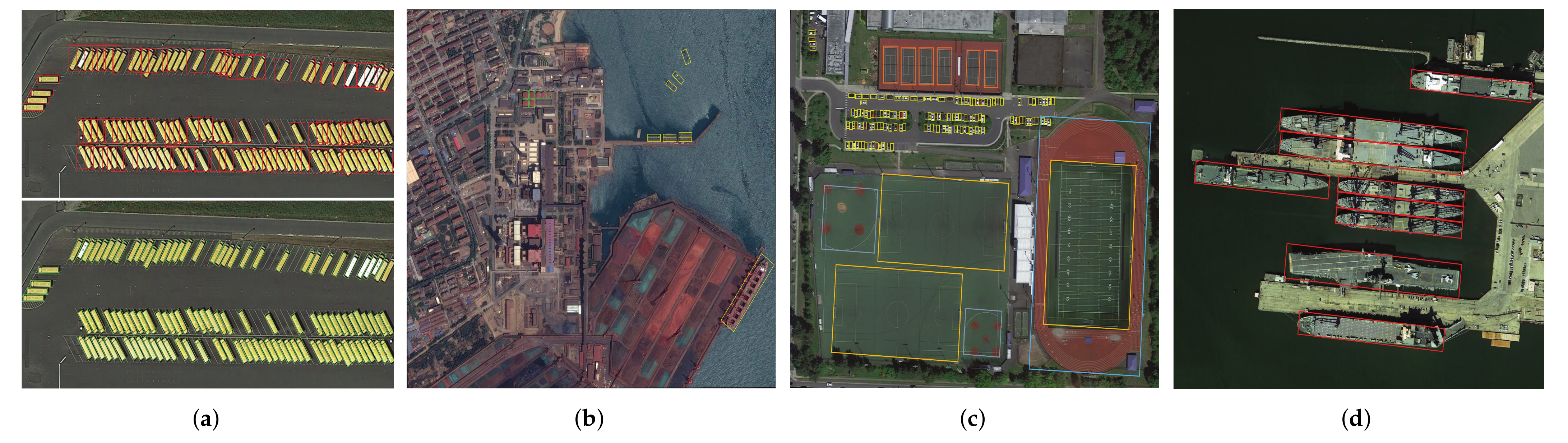
In recent years, due to their outstanding learning abilities, the most advanced detection models have been developed by using deep convolutional neural networks (DCNNs). Existing natural image object detection approaches [7,8,9,10,11,12,13,14,15,16,17,18] usually leverage the horizontal detection paradigm, which has evolved into a well-established area. Nevertheless, remote sensing images are typically taken with bird’s-eye views, and horizontal-detection-based methods will experience significant performance degradation when applied directly to remote sensing images, largely owing to the distinctive appearances and characteristics of remote sensing objects. For instance, compared with the detection of objects in images of natural scenes, the task of remote sensing object detection tends to encompass more challenges, such as complex backgrounds, arbitrary orientations, multi-scale distributions, and large aspect ratio variations. When we take the horizontal bounding box (HBB) in the top half of Figure 1a to represent the objects of a remote sensing image, it will introduce massive numbers of extra pixels outside of the targets, seriously damaging the accuracy of positioning. Meanwhile, the HBB used for densely arranged remote sensing oriented objects may generate a larger intersection-over-union (IoU) with adjacent boxes, which tends to introduce some missed ground-truth boxes that are restrained by non-maximum suppression (NMS), and the missed detection rate increases. To tackle these challenges, oriented object detection methods that utilize an oriented bounding box (OBB) to compactly enclose an object with orientations are preferred in RSIs.

Figure 1.
Some RSIs in the DOTA and HRSC2016 datasets. (a) The direction of objects in RSIs is always arbitrary. The HBB (top) and OBB (bottom) are two representation methods in RSI object detection. (b) Remote sensing images tend to contain complex backgrounds. (c) The scales of objects in the same remote sensing image may also vary dramatically, such as with small vehicles and track fields on the ground. (d) There are many objects with large aspect ratios in RSIs, such as slender ships.
Existing oriented object detectors are mainly inherited from the anchor-based detection paradigm. Nevertheless, anchor-based oriented object detectors that rely on anchor mechanisms result in complicated computations and designs related to the rotated anchor boxes, such as those of the orientations, scales, number, and aspect ratios of the anchor boxes. Therefore, research works on anchor-free detection methods that liberate the detection model from massive computations on the anchors have drawn much attention in recent years. Specifically, as an active topic in the field of anchor-free object detection, keypoint-based methods (e.g., CornerNet [13], CenterNet [14], and ExtremeNet [15]) propose forsaking the design of anchors and directly regressing target positions by exploring the features of correlative keypoints either on the box boundary points or the center point. To the best of our knowledge, many works that were built upon the keypoint-based detection pipeline have achieved great success in the RSI object detection field. For example, P-RSDet [19] converted the task of detection of remote sensing targets into the regression of polar radii and polar angles based on the center pole point in polar coordinates. GRS-Det [20] proposed an anchor-free center-based ship detection algorithm based on a unique U-shape network design and a rotation Gaussian Mask. The VCSOP detector [21] transformed the vehicle detection task into a multitask learning problem (i.e., center, scale, orientation, and offset subtasks) via an anchor-free one-stage fully convolutional network (FCN). Due to the bird’s-eye views in RSIs, center-based methods that have fewer ambiguous samples and vivid object representation are more suitable for remote sensing oriented object detection. Notably, center-based methods usually extend the CenterNet [14] to the oriented object detection task by introducing an accessional angle together with the width w and height h. However, due to the periodicity of the angle, angle-based approaches that represent the oriented object with the angle-oriented OBB will encounter boundary discontinuity and regression uncertainty issues [22], resulting in serious damage to the detection performance. To address this problem, our work explores an angle-free method according to the geometric characteristics of the OBB. Specifically, we describe an OBB as a center-based rotated inscribed ellipse (RIE), and then employ six parameters to describe the RIE inside each OBB: the center point position of the RIE (center point ), the offsets of the long half axis (), the length of the short half axis b, and an orientation label . In contrast to the angle-based approaches, our angle-free OBB definition guarantees the uniqueness of the representation of the OBB and effectively eliminates the boundary case, which dramatically improves the detection accuracy.
On the other hand, trapped by the complicated backgrounds and multi-scale object distribution in RSIs, as shown in Figure 1b,c, keypoint-based detectors that utilize a single-scale high-resolution feature map to make predictions may detect a large number of uninteresting objects and omit some objects with multiple scales. Therefore, it is momentous to enhance the feature extraction capability and improve the multi-scale information fusion of the backbone network. In our work, we design a high-resolution gated aggregation network (HRGANet) that better distinguishes the objects of interest from complex backgrounds and integrates the features with different scales by using a parallel multi-scale information interaction and gated aggregation information fusion mechanisms. In addition, because large aspect ratios tend to make a significant impact on the orientation error and the accuracy of the IoU, it is reasonable to assign penalties on the orientation loss based on the aspect ratio information. Taking the perspective that the eccentricity of the RIE can better reflect the aspect ratio from the side, we propose an eccentricity-wise orientation loss (ewoLoss) to penalize the orientation loss based on the eccentricity of the RIE, which effectively takes into consideration the effect of the aspect ratio on the orientation error and improves the accuracy of the detection of slender objects.
In summary, the contributions of this article are four-fold:
- We introduce a novel center-based OBB representation method called the rotated inscribed ellipse (RIE). As an angle-free OBB definition, the RIE effectively eliminates the angle periodicity and address the boundary case issues;
- We design a high-resolution gated aggregation network to capture the objects of interest from complicated backgrounds and integrate different scale features by implementing multi-scale parallel interactions and gated aggregation fusion;
- We propose an eccentricity-wise orientation loss function to fix the sensitivity of the eccentricity of the ellipse to the orientation error and effectively improve the accuracy of the detection of slender oriented objects with large aspect ratios;
- We perform extensive experiments to verify the advanced performance compared with state-of-the-art oriented object detectors on remote sensing datasets.
The rest of this article is structured as follows. Section 2 introduces the related work in detail. The detailed introduction of our method is explained in Section 3. In Section 4, we explain the extensive comparison experiments, the ablation study, and the experimental analysis at length. Finally, the conclusion is presented in Section 5.
2. Related Works
In this section, relevant works concerning deep-learning-based oriented object detection methods and anchor-free object detection methods in RSIs are briefly reviewed.
2.1. Oriented Object Detection in RSIs
Considering the rotation characteristics of remote sensing objects, it is more suitable to employ a rotated bounding box to represent objects with multiple orientations and to devise advanced oriented object detection algorithms that adapt to remote sensing scenes.
Recent advances in oriented object detection have mainly been driven by the improvements and promotion of general object detection methods that use horizontal bounding boxes to represent remote sensing objects. In general, the mainstream and classical oriented object detection algorithms in RSIs can be roughly divided into anchor-based paradigms and anchor-free object detection methods. The anchor-based detectors (e.g., YOLO [10], SSD [11], Faster-RCNN [9], and RetinaNet [12]) have dominated the field of object detection for many years. Specifically, for a remote sensing image, the anchor-based detectors first utilize many predetermined anchors with different sizes, aspect ratios, and rotation angles as a reference. Then, the detector either directly regresses the location of the object bounding box or generates region proposals on the basis of anchors and determines whether each region contains some category of an object. Inspired by this kind of ingenious anchor mechanism, a large number of oriented object detectors [22,23,24,25,26,27,28,29,30,31,32,33,34,35,36,37,38,39,40,41] have been proposed in the literature to pinpoint oriented objects in RSIs. For example, Liu et al. [23] used the Faster-RCNN framework and introduced a rotated region of interest (ROI) for the task of the detection of oriented ships in RSIs. The method in [24,25] used a rotation-invariant convolutional neural network to address the problem of inter-class similarity and intra-class diversity in multi-class RSI object detection. The RoI Transformer [30] employed a strategy of transforming from a horizontal RoI to an oriented RoI and allowed the network to obtain the OBB representation with a supervised RoI learner. With the aim of application for rotated ships, the PN [31] transformed the original region proposal network (RPN) into a rotated region proposal network (PN) to generate oriented proposals with orientation information. CAD-Net [32] used a local and global context network to obtain the object-level and scene contextual clues for robust oriented object detection in RSIs. The work in [33] proposed an iterative one-stage feature refinement detection network that transformed the horizontal object detection method into an oriented object detection method and effectively improved the RSI detection performance. In order to predict the angle-based OBB, SCRDet [34] applied an IoU penalty factor to the general smooth L1 loss function, which cleverly addressed the angular periodicity and boundary issues for accurate oriented object detection tasks. A-Net [35] realized the effect of feature alignment between the horizontal features and oriented objects through an one-stage fully convolutional network (FCN).
In addition to effective feature extraction network designs for oriented objects mentioned above, some scholars have studied the sensitivity of angle regression errors to anchor-based detection methods and resorted to more robust angle-free OBB representations for oriented object detection in RSIs. For instance, Xu et al. [36] represented an arbitrarily oriented object by employing a gliding vertex on the four corners based on the HBB, which refrained from the regression of the angle. The work in [37] introduced a two-dimensional vector to express the rotated angle and explored a length-independent and fast IoU calculation method for the purpose of better slender object detection. Furthermore, Yang et al. [22] transformed the task of the regression of an angle into a classification task by using an ingenious circular smooth label (CSL) design, which eliminated the angle periodicity problem in the process of regression. As a continuation of the CSL work, densely coded labels (DCLs) [38] were used to further explore the defects of CSLs, and a novel coding mode that made the model more sensitive to the angular classification distance and the aspect ratios of objects was proposed. ProjBB [39] addressed the regression uncertainty issue caused by the rotation angle with a novel projection-based angle-free OBB representation approach. Not singly, but in pairs, the purpose of our work is also to explore an angle-free OBB representation for better oriented object detection in remote sensing images.
2.2. Anchor-Free Object Detection in RSIs
Recently, as an active theme in the field of remote sensing object detection, anchor-free methods have been put forward to abandon the paradigm of anchors and to regress the bounding box directly through a sequence of convolution operations. In general, anchor-free methods can be classified into per-pixel point-based detectors and keypoint-based detectors. The per-pixel point-based detectors (e.g., DenseBox [16], FoveaBox [17], and FCOS [18]) detect objects by predicting whether a pixel point is positive and the offsets from the corresponding per-pixel point to the box boundaries of the target. DenseBox [16] first attempted to employ an anchor-free pipeline to directly predict the classification confidence and bounding box localization with an FCN. FCOS [18] detected an object by predicting four distances from pixel points to four boundaries of the bounding box. Meanwhile, FCOS also introduced a weight factor, Centerness, to evaluate the importance of the positive pixel points and steer the network to distinguish discriminative features from complicated backgrounds. FoveaBox [17] located the object box by directly predicting the mapping transformation relation between center points and two corner points, and it learned the object category of confidence. Inspired by this paradigm of detection, many researchers began to explore per-pixel point-based oriented object detection approaches for RSIs. For example, based on the FCOS pipeline, IENet [42] proposed an interacting module in the detection head to bind the classification and localization branches for accurate oriented object detection in RSIs. In addition, IENet also introduced a novel OBB representation method that depicted oriented objects with an outsourcing box of the OBB. Axis Learning [43] used a per-pixel point-based detection model that detected the orientated objects by predicting the axis of an object and the width perpendicular to the axis.
Differently from per-pixel point-based methods, keypoint-based methods (e.g., CornerNet [13], CenterNet [14], and ExtremeNet [15]) pinpoint oriented objects by capturing the correlative keypoints, such as the corner point, center point, and extreme point. CornerNet is the forerunner of the keypoint-based methods; it locates the HBB of an object through heatmaps of the upper-left and bottom-right points. It groups the corner points of the box by evaluating the embedding distances. CenterNet captures an object by using a center keypoint and regressing the width, height, and offset properties of the bounding box. ExtremeNet detects an object through an extreme point (extreme points of four boundaries) and center point estimation network. In the remote sensing oriented object detection field, many works have based themselves upon the keypoint-based detection framework. For example, combining CornerNet and CenterNet, Chen et al. [44] utilized an end-to-end FCN to identity an OBB according to the corners, center, and corresponding angle of a ship. CBDA-Net [45] extracted rotated objects in RSIs by introducing a boundary region and center region attention module and used an aspect-ratio-wise angle loss for slender objects. The work in [46] proposed a pixel-wise IoU loss function that enhances the relation between the angle offset and the IoU and effectively improves the detection performance for objects with high aspect ratios. Pan et al. [47] introduced a unified dynamic refinement network to extract densely packed oriented objects according to the selected shape and orientation features. Meanwhile, there are also some works that have integrated the angle-free strategy into the keypoint-based detection pipeline for RSIs. -DNet [48] utilized a center point detection network to locate the intersection point and formed an OBB representation with a pair of internal middle lines. X-LineNet [49] detected aircraft by predicting and clustering the paired vertical intersecting line segments inside each bounding box. BBAVectors [50] captured an oriented object by learning the box-boundary-aware vectors that were distributed in four independent quadrants of the Cartesian coordinate system. Continuing this angle-free thought, the method proposed in this article uses a center-based rotated inscribed ellipse to represent the OBB. At the same time, our method provides a strong feature extraction network to extract objects from complex backgrounds and implements an aspect-ratio-wise orientation loss for slender objects, which effectively boosts the performance in oriented object detection in RSIs. A more detailed introduction of the proposed method will be provided in Section 3.
3. Materials and Methods
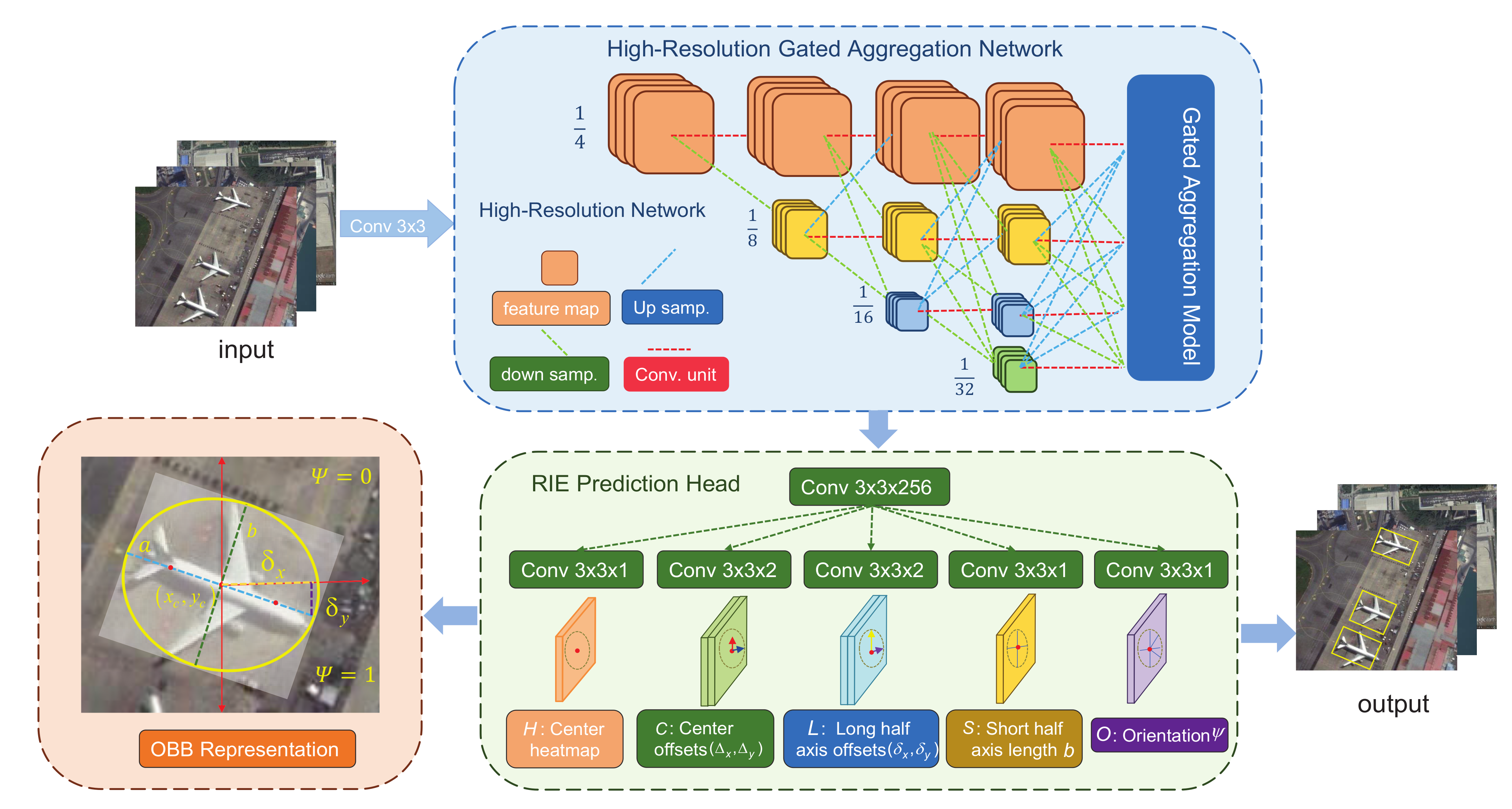
The architecture of the proposed method is illustrated in Figure 2. The network framework mainly includes a feature extraction network—namely, a high-resolution gated aggregation network (HRGANet) and a multitask prediction head. The HRGANet is designed to tackle the problems of extensive multi-scale distributed objects and complex backgrounds in RSIs. The HRGANet can be divided into the backbone, the high-resolution network (HRNet) [51], and the gated aggregation model. The HRNet is a parallel-interaction high-resolution network that is utilized to fuse multi-resolution feature representations and render high-resolution representations for richer semantic information and more precise spatial positioning information. The gated aggregation module (GAM) is proposed to adaptively fuse different resolution feature maps for multi-scale objects through a gated aggregation mechanism. Meanwhile, there are five subnetworks for the center heatmap, center offset, long half-axis offset, eccentricity, and orientation prediction in the oriented object detection head. Finally, oriented objects are detected by predicting the inscribed ellipse with orientation information inside each OBB. In addition, we utilize ewoLoss to penalize the orientation loss based on the eccentricity of the rotated inscribed ellipse for better slender object detection. We will introduce the network from three perspectives: (1) the high-resolution gated aggregation network; (2) the rotated inscribed ellipse prediction head; (3) the eccentricity-wise orientation loss.

Figure 2.
Framework of the our method. The backbone network, HRGANet, is followed by the RIE prediction model. The HRGANet backbone network contains HRNet and GAM. Up samp. represents a bilinear upsampling operation and a 1 × 1 convolution. Down samp. denotes 3 × 3 convolution with a stride of 2. Conv unit. is a 1 × 1 convolution.
3.1. High-Resolution Gated Aggregation Network
As illustrated in Section 1, the objects in remote sensing images tend to have the characteristics of large-scale variations and complicated backgrounds. Therefore, it is necessary to design an effective feature extraction network that fully exploits the multi-resolution feature representations and fuses multi-scale information for robust multi-scale feature extraction. From this point of view, we introduce a high-resolution gated aggregation network (HRGANet) to make good use of the multi-resolution feature maps. As shown in Figure 2, the HRGANet is composed of two components: the high-resolution network (HRNet) and gated aggregation model (GAM).
3.1.1. High-Resolution Network
The backbone network for feature extraction in our method uses HRNet, which performs well in keypoint detection. In contrast to the frequently used keypoint extraction networks (e.g., VGG [52], ResNet [53], and Hourglass [54]) that concatenate the multi-resolution feature maps in series, HRNet links different-resolution feature maps in parallel with repeated multi-scale fusion. The whole procedure of keypoint extraction in HRNet efficiently keeps high-resolution features while replenishing the high- and low-resolution information, which enables it to obtain abundant multi-scale feature representations. The brief sketch of HRNet is illustrated in Figure 2. First, the input image is fed into a stem, which consists of two 3 × 3 convolutions with a stride of 2. Then, the resolution is decreased to 1/4. The overall structure of HRNet has four main stages, which gradually add high-to-low resolution stages in succession. The structure of these four stages can be simplified, as indicated in the following formula:
where represents the ith sub-stage and denotes that the resolution of feature maps in the corresponding sub-stage is of the original feature maps. Meanwhile, through repeated multi-resolution feature fusion and parallel high-resolution feature maintenance, HRNet can better extract multi-scale features, and then obtain richer semantic and spatial information for RSI objects. The detailed network structure of HRNet is shown in Table 1. Note that we used HRNet-W48 in our experiments.

Table 1.
The structure of the backbone network of HRNet. It mainly embodies four stages. The 1st (2nd, 3rd, and 4th) stage is composed of 1 (1, 4, and 3) repeated modularized blocks. Meanwhile, each modularized block in the 1st (2nd, 3rd, and 4th) stage consists of 1 (2, 3, and 4) branch(es) belonging to a different resolution. Each branch contains four residual units and one fusion unit. In the table, each cell in the Stage box is composed of three parts: The first part represents the residual unit, the second number denotes the iteration times of the residual units, and the third number represents the iteration times of the modularized blocks. ≡ in the Fusion column represents the fusion unit. C is the channel number of the residual unit. We set C to 48 and represent the network as HRNet-W48. Res. is the abbreviation of resolution.
3.1.2. Gated Aggregation Model
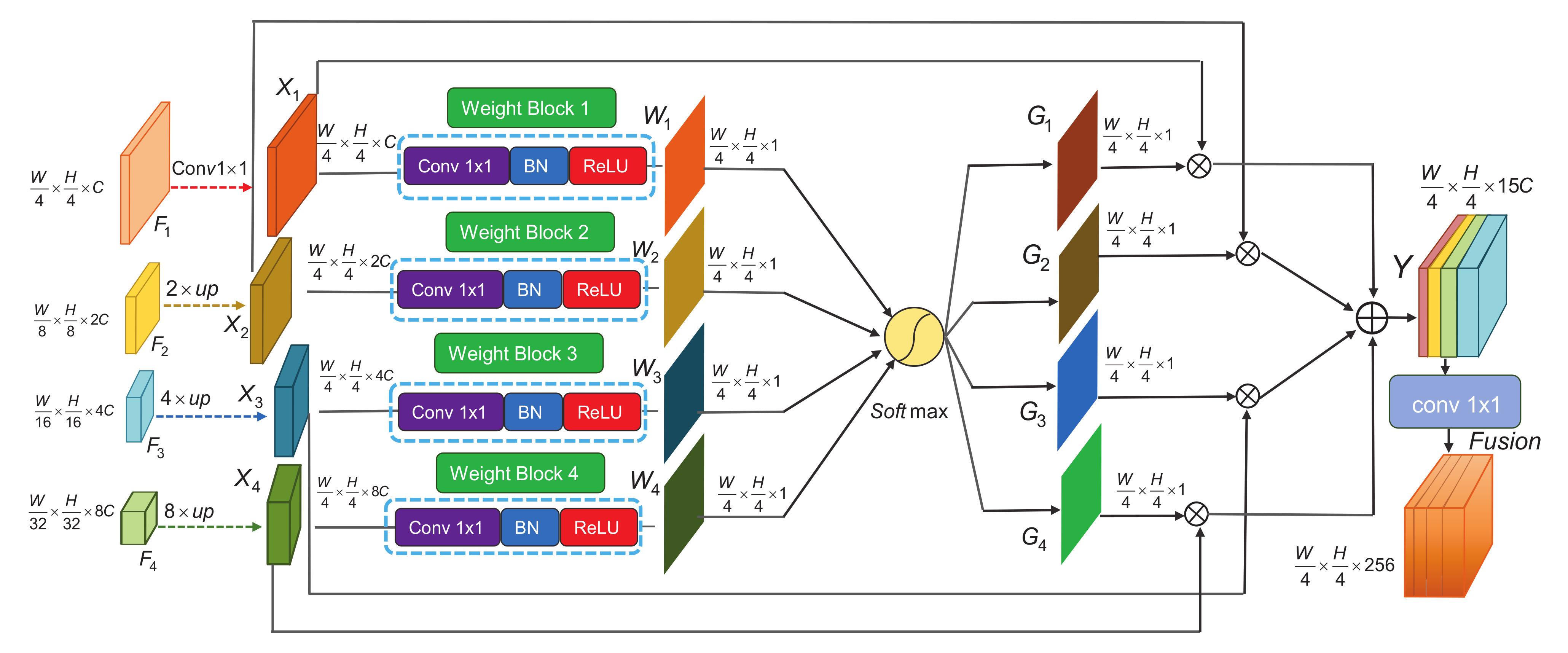
In a conventional keypoint or object detection network, the feature aggregation pattern is carried out by directly stacking or concatenating the feature maps. Nevertheless, to the best of our knowledge, feature maps with different resolutions contain serious semantic dissimilarities. In general, low-resolution feature maps provide richer semantics for object category recognition, whereas high-resolution feature maps contain more spatial information for object localization. Some works [21,50] directly up-sampled low-resolution feature maps (, , and feature maps) to a spatial resolution, and then fused these feature maps through a concatenation operation. This kind of fusion strategy does not consider that some of these features are meaningless or a hindrance to the inference of object identification and positioning. To enhance valuable feature representations and restrain invalid information, we designed a gated aggregation mechanism (GAM) to evaluate the availability of pixels in each feature map and effectively fuse multi-resolution feature representations. The details of the GAM are presented in Figure 3. As shown in Figure 2, the inputs of the GAM are the output feature maps of the HRNet, where W, H, and C represent the width, height, and channel number of the feature maps, respectively. In Figure 3, , , and are up-sampled to the same resolution as . We can obtain the feature maps of the same scale . Then, is fed into a weight block to adaptively assign the weight of pixels in different feature maps and to generate the weight maps . can be defined as
where represents the convolution operation in which the number of kernels is equal to 1, denotes the batch normalization operation, and is the ReLU activation function. These three parts compose a weight block. Then, we employ a SoftMax operation to obtain the normalized gate maps as:
where is the important gated aggregation factor. Finally, by means of these gate maps, the gated aggregation feature maps output for the following prediction head, which can be calculated as:
where the summation symbol represents the concatenation operation ⊕. The feature maps are concatenated along the channel direction. Note that we perform a 1 × 1 convolution to reconcile the final feature maps and integrate the feature maps into the 256 channels after Y. With this gated aggregation strategy, meritorious feature representations are distributed to higher gate factors, and unnecessary information will be suppressed. As a result, our feature extraction network can provide more flexible feature representations in detecting remote sensing objects of different scales from complicated backgrounds.

Figure 3.
The network structure of the GAM. W, H, and C represent the width, height, and channel number of the feature maps, respectively. ⊗ represents the broadcast multiplication operation. ⊕ denotes the concatenation operation. is a convolution operation with 1 × 1 kernels, BN is a batch normalization operation, and ReLU is the ReLU activation function. A weight block is composed of a 1 × 1 convolution operation, a BN operation, and a ReLU operation.
3.2. Rotated Inscribed Ellipse Prediction Head
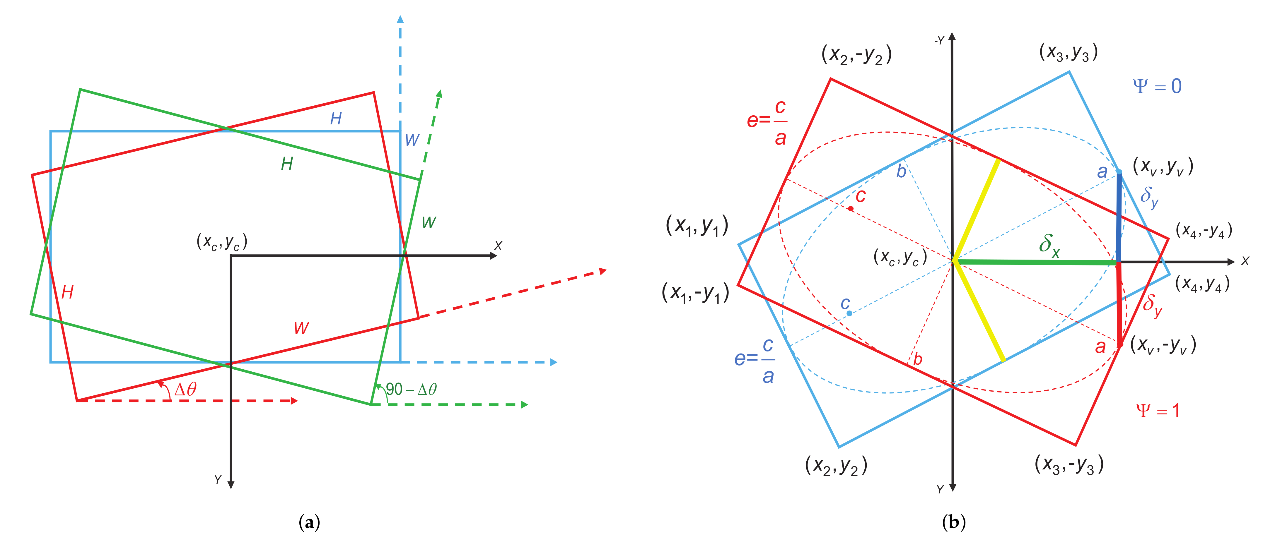
To capture the objects in RSIs, some works [21,45] described the OBB with a rotated rectangular box (RRB) representation . As shown in Figure 4a, x, y, w, h, and represent the center abscissa, center ordinate, width, height, and angle. This representation method has some pros and cons. On the bright side, this definition method can ensure the conciseness and uniqueness of the OBB representation. Nevertheless, there still exist some problems in some extreme conditions. For example, in Figure 4a, the rotation angle of the RRB is defined as the angle between the horizontal axis (x-axis) corresponding to the lowest point of the RRB and the first edge encountered when it rotates counterclockwise. The first edge encountered is the width and the other is the height, which are not defined in terms of length. This angular representation has a range of angles of . However, a boundary problem emerges due to the angular periodicity when this representation encounters an angular boundary. In Figure 4a, the blue rectangle denotes the angle , which is equal to 0. When this rectangle is subjected to a slight jiggle, two very different conditions appear. When we rotate the blue box by a small angle towards the upper-right corner to reach the position of the red box, the angle of rotation is defined as . However, when we rotate the blue box by a small angle towards the bottom-right corner to reach the position of the green box, the angle of rotation is defined as . This kind of rotation angle representation method causes a large jump in the angle’s value during the rotation of the rectangular box from the top-right corner to the bottom-right corner, and the regression of the angle parameter is discontinuous and has serious jitter problems. In addition, for the red box, the long side is the width and the short side is the height. However, for the green box, the short side is the width and the long side is the height. For these two boxes in close proximity, the width and height are abruptly swapped, which makes the regression in terms of width and height less effective. In this condition, a tiny change in the rotation angle would lead to a large change in the regression target, which seriously hinders the training of the network and deteriorates the performance of the detector.

Figure 4.
(a) RRB representation , where , w, h, and represent the center point, width, height, and small angle jitter, respectively. (b) RIE representation of the target used in our method. , , and are the center point, long half-axis vertex, and four outer rectangle vertices of the RIE. e and represent the eccentricity and orientation label, respectively. Yellow lines b denote the short half axis. Red, blue, and green lines represent the offsets of the long half axis a.
To address the above-mentioned problems, we propose a new angle-free OBB representation. We transform the OBB regression task into the corresponding RIE regression problem. First, as shown in Figure 4b, we represent the OBB as four vertices , where the order of the four vertices is based on the values of , i.e., . Then, we can calculate the coordinate of the long half-axis vertices . When is equal to , the bounding box is the HBB. The coordinates of the HBB’s long half-axis vertices are defined as:
where is the coordinate of the center point. Therefore, we can obtain the long half-axis offsets . By predicting the offsets between the long half-axis vertices and the center point, we can obtain the long half-axis length value . Meanwhile, to obtain the complete size of the RIE, we also implement a sub-network to predict the short half-axis length b. In addition, as shown in Figure 4b, it is not well established to represent a unique RIE by predicting the center point , long half-axis offsets , and short half axis b because there are two obscure RIEs with mirror symmetry on the x-axis. To remove this ambiguity, we design an orientation label , and the ground truth of is defined as:
When the long half-axis vertex is located in the 1st quadrant or y-axis, is equal to 0. Meanwhile, when the long half-axis vertex is located in the 4th quadrant or x-axis, is equal to 1. By using such a classification strategy, we can effectively ensure the uniqueness of the RIE representation and eliminate the ambiguity of the definition. Finally, the representation of the RIE can be described by a 6-D vector . As shown in Figure 2, we introduce an RIE prediction head to obtain the parameters of the RIE. First, a convolutional unit is employed to reduce the channel number of the gated aggregated feature maps Y to 256. Then, five parallel convolutional units follow to generate a center heatmap , a center offset map , a long half-axis offset map , a short-half axis length map , and an orientation map , where K is the number of categories of the corresponding datasets. Note that the output orientation map is finally processed by a sigmoid function. For the sake of brevity, we have not shown final sigmoid function in Figure 2.
3.3. Eccentricity-Wise Orientation Loss
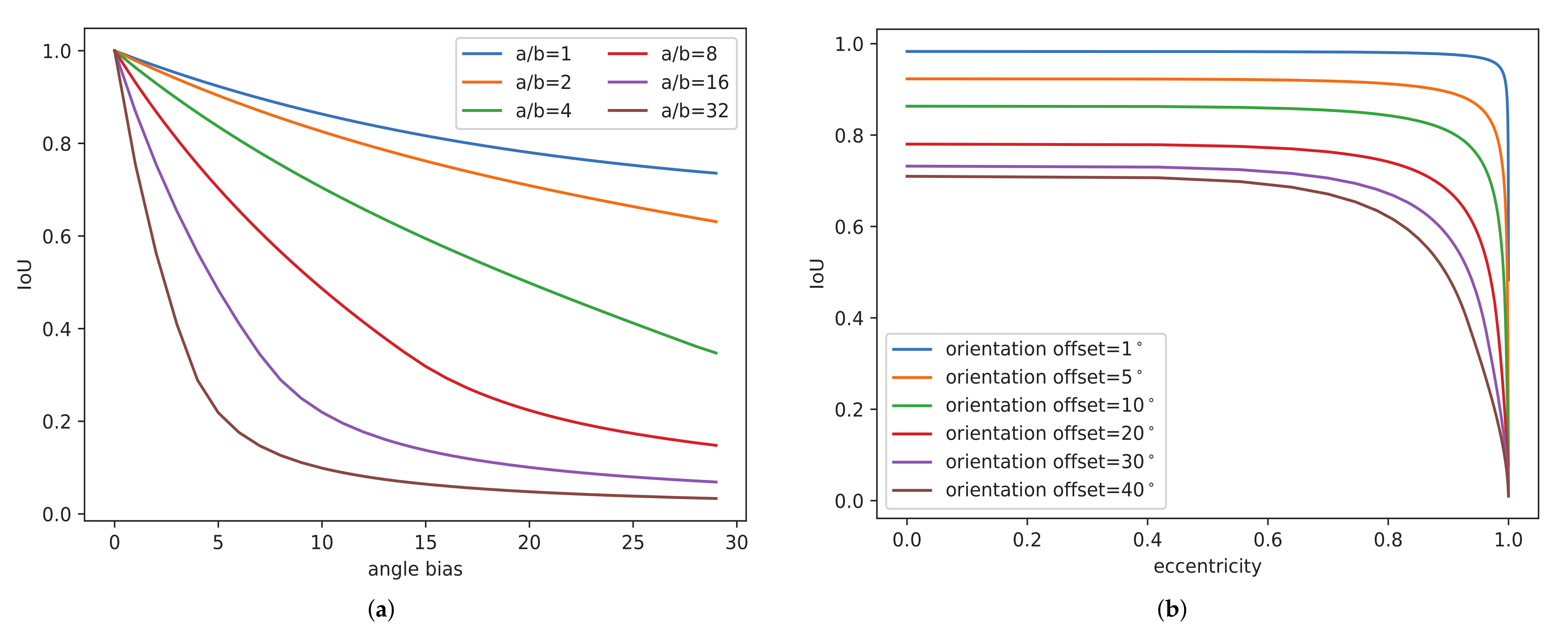
In addition to the characteristics of complex backgrounds, arbitrary orientations, and multi-scale distributions, large aspect ratio variations are also salient characteristics of RSI objects. For example, the aspect ratios of a baseball diamond and a storage tank in RSIs approach 1, but the aspect ratios of long and narrow objects, such as bridges and ships, are even higher than 50. Therefore, it is worthwhile to explore the effects of objects’ aspect ratios on the accuracy of the detection of rotated objects. As shown in Figure 5a, we first fix the width, height, and center point of the ground-truth rotated bounding box and the predicted rotated bounding box. Then, we record the IoU value between the ground truth and the predicted box with different angle biases and aspect ratios. We can see from the observation that the sensitivity of the IoU to the angle bias varies considerably for different aspect ratios. First, for the same aspect ratio, the IoU between two rotated boxes decreases as the angle bias increases. Meanwhile, under the same angle bias, the larger the aspect ratio is, the smaller the IoU is. That is, generally, more slender and narrow objects have greater sensitivity to angle deviations. For long and narrow objects, a small angle bias will lead to a large IoU variation. In addition, eccentricity is another important index that can reflect the degree of narrowness of an object. The narrower an object is, the larger the eccentricity is. As shown in Figure 5b, we also record the IoU values under different orientation offsets and the eccentricity of the RIE. Under the same orientation offsets, the larger the eccentricity is, the smaller the IoU is. To take full account of the effect of the aspect ratio on the angle prediction bias, we introduce an eccentricity-wise orientation loss (ewoLoss) that utilizes the eccentricity e of the RIE to represent the aspect ratio, and it effectively eliminates the influence of large aspect ratio variations on detection accuracy. First, we propose the utilization of the cosine similarity of the long half axis between the predicted RIE and the ground-truth RIE to calculate the orientation offset. Specifically, with the aid of the ground-truth long half-axis offsets and the predicted long half-axis offsets , we can calculate the orientation offset between the predicted long half axis and ground-truth long half axis:

Figure 5.
(a) IoU curves under different height–width ratios and angle biases. a/b represent the height–width ratio, i.e., the aspect ratio of the object. (b) IoU curves under different orientation offsets and RIE eccentricities.
denotes the inverse cosine function. indicates the angle error between the predicted RIE and ground-truth RIE. Then, considering that the orientation offsets under different eccentricities have varying influences on the performance of rotated target detection, we hope that the orientation losses under different eccentricities are different, and the orientation losses of targets with greater eccentricities should be larger. The ewoLoss is calculated as:
where i is the index value of the target, and represents the exponential function. is the eccentricity in object i, is a constant to modulate the orientation loss, and N is the object number in one batch.
3.4. Loss Functions
Our total loss function is a multi-task loss and is composed of five parts. The first part is the center heatmap loss. A heatmap is a commonly used technical tool applied to keypoint detection tasks in general images. In our work, we inherit the center point heatmap method from the CenterNet [14] network to detect the center points of oriented objects in RSIs. As described in Figure 2, the center heatmap in the RIE prediction head has K channels, with each belonging to one target category. The value of each predicted pixel point in the heatmap denotes the confidence of detection. We apply a 2-D Gaussian around the heatmap of the object’s center point to form the ground-truth heatmap , where denotes the pixel point in heatmap , and s represents the standard deviation of the adapted object size. Then, following the idea of CornerNet [13], we utilize the variant focal loss to train the regression of the center heatmap:
where and h represent the ground-truth and predicted values of the heatmap, N is the number of targets, and i denotes the pixel location in the heatmap. The hyper-parameters and are set to 2 and 4 in our method to balance the ratio of positive and negative samples. The second part of our loss is the center offset loss. Because the coordinates of the center keypoint on the heatmap are integer values, the ground-truth values of the heatmap are generated by down-sampling the input image through the HRGANet. The size of the ground-truth heatmap is reduced compared to that of the input image, and the discretization process will introduce rounding errors. Therefore, as shown in Figure 2, we introduce center offset maps to predict the quantization loss between the integer center point coordinates and quantified center point coordinates for the mapping of the center point from the input image to the heatmap:
Smooth loss is adopted to optimize the center offset as follows:
where N is the number of targets, and are the ground-truth and predicted values of the offsets, and k denotes the object index number. The smooth loss can be calculated as:
The third part of our loss is the box size loss. The box size is composed of the long half-axis offsets and the short half-axis length b. We describe the box size with a 3-D vector . We also use a smooth loss to regress the box size parameters:
where N is the number of targets, and are the ground-truth and predicted box size vectors, and k denotes the object index number. The fourth part of our loss is the orientation loss. As shown in Figure 2, we use an orientation label to determine the orientation of the RIE. We use the binary cross-entropy loss to train the orientation label loss as follows:
where N is the number of targets, and are the ground-truth and predicted orientation labels, and i denotes object index number. The last part is the eccentricity-wise orientation loss . Finally, we use the weight uncertainty loss [55] to balance the multi-task loss, and the final loss used in our method is designed as follows:
where , , , , and are the learnable uncertainty indexes for balancing the weight of each loss. The uncertainty loss can automatically learn the multitask weights from training data. The detailed introduction of this multitask loss can be found in [55].
4. Experiments and Analysis of the Results
In this section, we first introduce two public remote sensing image datasets, DOTA [56] and HRSC2016 [57], as well as the evaluation metrics used in our experiments. Then, we analyze the implementation details of the network training and the inference process of our detector. Next, we analyze the experimental results on two datasets in comparison with the state-of-the-art detectors. Finally, some ablation study results and promising detection results are displayed.
4.1. Datasets
4.1.1. DOTA
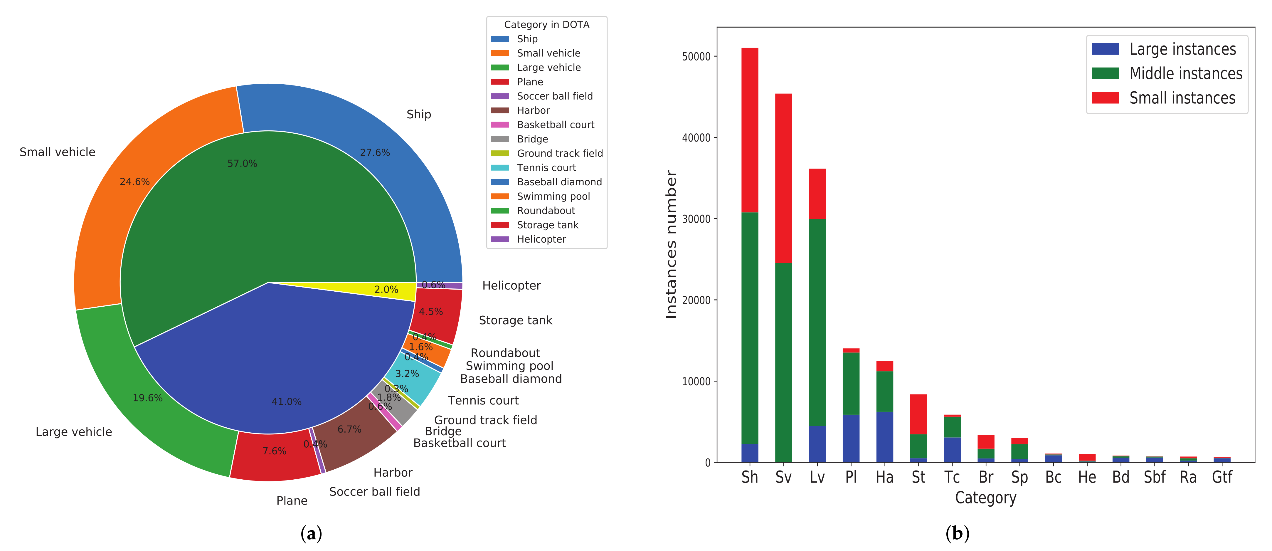
DOTA [56] is composed of 2806 remote sensing images and 188,282 instances in total. Each instance is annotated with oriented bounding boxes consisting of four vertex coordinates, which are collected from multiple sensors and platforms. The images of this dataset mainly contain the following categories: storage tank (ST), plane (PL), baseball diamond (BD), tennis court (TC), swimming pool (SP), ship (SH), ground track field (GTF), harbor (HA), bridge (BR), small vehicle (SV), large vehicle (LV), roundabout (RA), helicopter (HC), soccer-ball field (SBF), and basketball court (BC). In Figure 6, we present the proportion distribution of numbers and the size distribution of the instances of each category in the DOTA dataset. We can see that this multi-class dataset contains a large number of multi-scale oriented objects in RSIs with complex backgrounds, so it is suitable for experiments. In the DOTA dataset, the splits of the training, validation, and test sets are 1/2, 1/6, and 1/3, respectively. The size of each image falls within the range of 0.8 k × 0.8 k to 4 k × 4 k pixels. The median aspect ratio of the DOTA dataset is close to 2.5, which means that the effects of various aspect ratios on the detection accuracy can be well evaluated.

Figure 6.
(a) The proportion distribution of the numbers of instances in each category in the DOTA dataset. The outer ring represents the number distribution of 15 categories. The internal ring denotes the total distribution of small (green), middle (blue), and large instances (yellow). (b) The size distribution of instances in each category in the DOTA dataset. We divided all of the instances into three splits according to their OBB height: small instances for heights from 10 to 50 pixels, middle instances for heights from 50 to 300 pixels, and large instances for heights above 300 pixels.
4.1.2. HRSC2016
HRSC2016 [57] is a challenging dataset developed for the detection of oriented ship objects in the field of remote sensing imagery. It is composed of 1070 images and 2970 instances in various scales, orientations, and appearances. The image scales range from 300 × 300 to 1500 × 900 pixels, and all of the images were collected by Google Earth from six famous ports. The median aspect ratio of the HRSC2016 dataset approaches 5. The training, validation, and test sets contain 436, 181, and 444 images, respectively. In the experiments, both the training set and validation set were utilized for network training.
4.2. Evaluation Metrics
In this article, three common evaluation metrics—the mean average precision (mAP), F1 score, and frames per second (FPS)—were adopted to evaluate the accuracy and speed of the oriented object detection methods. First, two fundamental evaluation metrics, precision and recall, are indispensable before calculating the metric of the mAP. The precision metric represents the ratio of true positive samples to all positive samples. The recall metric denotes the ratio of true positive samples to all predicted positive samples. They are defined as follows:
where , , and represent the number of predictions of true positive samples, the number of predictions of false positive samples, and the number of predictions of false negative samples. In addition to the precision and recall, we can obtain the comprehensive evaluation metric, the F1 score, which is used for single-category object detection.
Meanwhile, utilizing the precision and recall, we can calculate the corresponding average precision (AP) in each category. By calculating the AP values of all of the categories, we obtain the mean AP (i.e., mAP) value for multi-class objects as follows:
where indicates the number of categories in the multi-class dataset (e.g., 15 for the DOTA dataset). and denote the precision and recall rates of the i-th class of predicted multi-class objects in the dataset. In addition, we use a general speed evaluation metric, FPS, which is calculated with the number of images that can be processed per second in order to measure the speed of object detection.
4.3. Implementation Details
The experimental environment of the proposed method was implemented with the PyTorch [58] deep learning framework. For the DOTA and HRSC2016 datasets, we cropped the input image resolution to 800 × 800 pixels and 512 × 512 pixels, respectively. We applied data augmentation strategies to enrich the datasets in the network training process, which included random rotation, random flipping, color jittering, and random scaling in the range of . We trained the network on two NVIDIA GTX 1080 Ti GPUs with a batch size of 8 and utilized Adam [59] with an initial learning rate of to optimize the network. In total, we trained the network for 120 epochs on the DOTA dataset and 140 epochs on the HRSC2016 dataset. The learning rate was reduced by a learning rate decay factor of 10 after the 80th and 100th epochs.
4.4. Network Inference
During network inference, the peaks in the heatmap are extracted as the center points for each class object by applying an NMS operation ( max-pooling operation). The heatmap value is considered as the detected category confidence score. When the category confidence score is higher than 0.1, it is considered as a correct object center point. Then, we take out the predicted center offsets , long half-axis offsets , the short half axis b, and the orientation label at the selected heatmap center point . We first add the center offsets to adjust the heatmap center point and obtain the modified heatmap center point . Finally, we can obtain the predicted rescaled center point location in the input image. The coordinates for four vertexes of the predicted RIE at the center point of can be formulated as follows:
where is an orientation guiding factor, and is defined as follows:
where denotes the predicted orientation label value. In addition, in the post-processing stage, there is still a large number of highly overlapping oriented boxes, which improves the false detection rate. In this situation, we employed the oriented NMS strategy from [21] to calculate the IoU between two OBBs and filter out the redundant boxes.
4.5. Comparison with State-of-the-Art Methods
In our experiments, to verify the effectiveness of our method, we compared it with state-of-the-art detectors on the task of oriented object detection in two remote sensing datasets: the DOTA [56] dataset and the HRSC2016 [57] dataset.
4.5.1. Results on DOTA
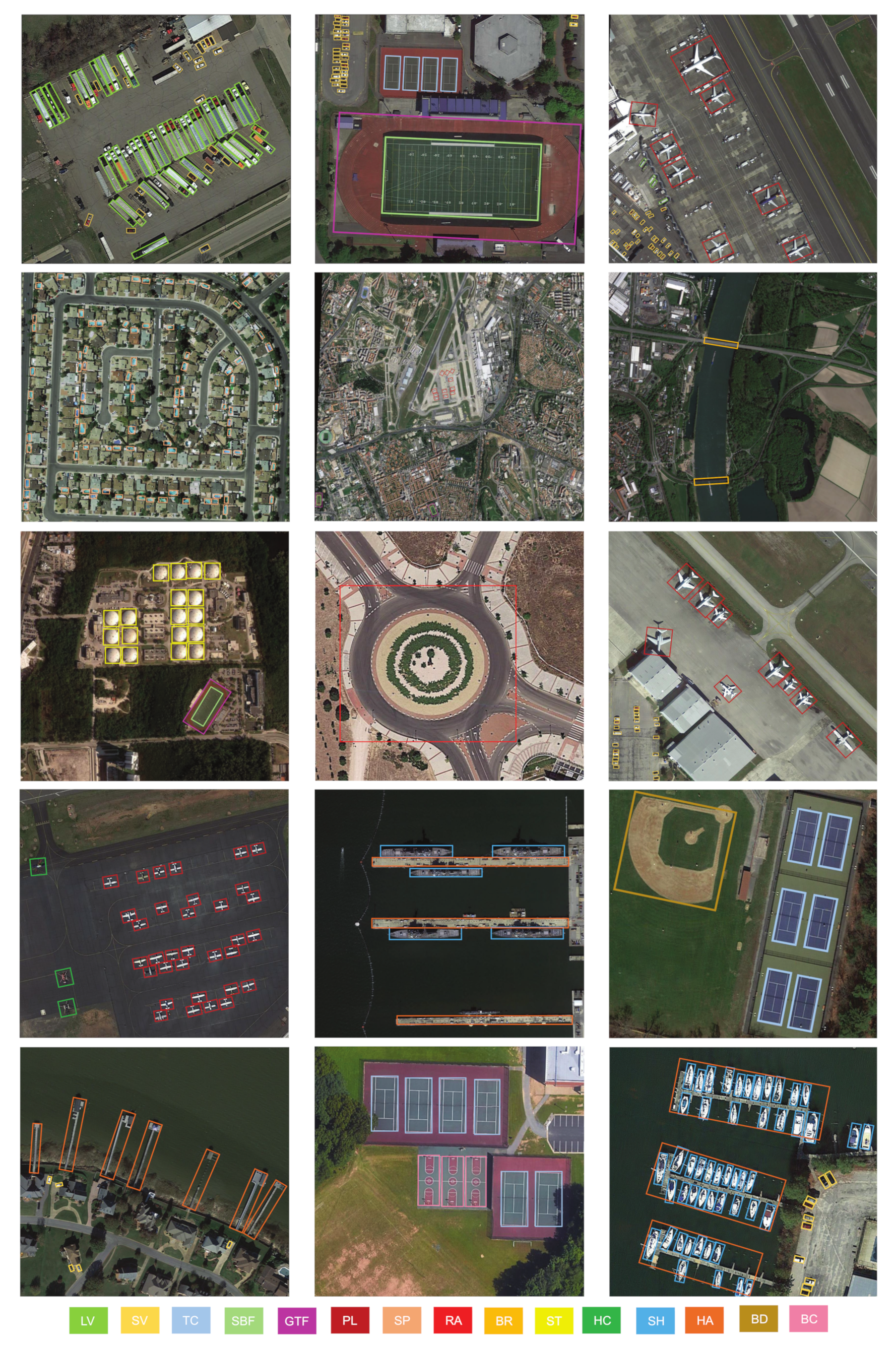
We compared our method with state-of-the-art anchor-based and anchor-free methods on the DOTA dataset. The results of the comparison of precision on the DOTA dataset are presented in Table 2. For a fair comparison, data augmentations were adopted for all of the compared methods. First, we compared the AP in fifteen categories of objects in the DOTA dataset and the mAP values of fourteen anchor-based detectors. FR-O [56] is the official baseline method proposed in the DOTA dataset. Based on the Faster-RCNN [9] framework, R-DFPN [26] adds a parameter of angle learning and improves the accuracy of the baseline from 54.13% to 57.94%. CNN [27] proposes a multi-scale regional proposal pooling layer followed by a region proposal network and boosts the accuracy to 60.67%. RRPN [28] introduces a rotating region of interest (RROI) pooling layer and realizes the detection of arbitrarily oriented objects, which improves the performance from 60.67% to 61.01%. ICN [29] designs a cascaded image network to enhance the features based on the R-DFPN [26] network and improves the performance of detection from 61.01% to 68.20%. Meanwhile, we report the detection results of nine other advanced oriented object detectors that were mentioned above, i.e., RoI Trans [30], CAD-Net [32], Det [33], SCRDet [34], ProjBB [39], Gliding Vertex [36], APE [37], A-Net [35], and CSL [22]. It can be noticed that our method of the RIE with the backbone of HRGANet-W48 obtained a 75.94% mAP and outperformed most of the anchor-based methods with which it was compared, except for A-Net [35] (76.11%) and CSL [22] (76.17%). In comparison with the official baseline of DOTA (FR-O [56]), the improvement in accuracy was 21.81%, which demonstrates the advantage of the RIE. Meanwhile, it is worth noting that the use of the RIE under HRGANet-W48 outperformed all of the reported anchor-free methods. Specifically, the RIE outperformed IENet [42], PIoU [46], Axis Learning [43], P-RSDet [19], -DNet [48], BBAVector [50], DRN [47], and CBDA-Net [45] by 18.8%, 15.44%, 9.96%, 6.12%, 4.82%, 3.62%, 2.71%, and 0.2% in terms of mAP. Moreover, the best and second-best AP values for detection in 15 categories of objects are recorded in Table 2. Our method achieved the best performance on objects with large aspect ratios, such as the large vehicle (LV) and harbor (HA), and the second-best performance on the baseball diamond (BD), bridge (BR), and ship (SH) with complicated backgrounds. In addition, we present the visualization of the detection results for the DOTA dataset in Figure 7. The detection results in Figure 7 indicate that our method can precisely capture multi-class and multi-scale objects with complex backgrounds and large aspect ratios.
Table 2.
Comparison with state-of-the-art methods of oriented object detection in RSIs on the DOTA dataset. We set the IoU threshold to 0.5 when calculating the AP.

Figure 7.
Visualization of the detection results of our method on the DOTA dataset.
4.5.2. Results on HRSC2016
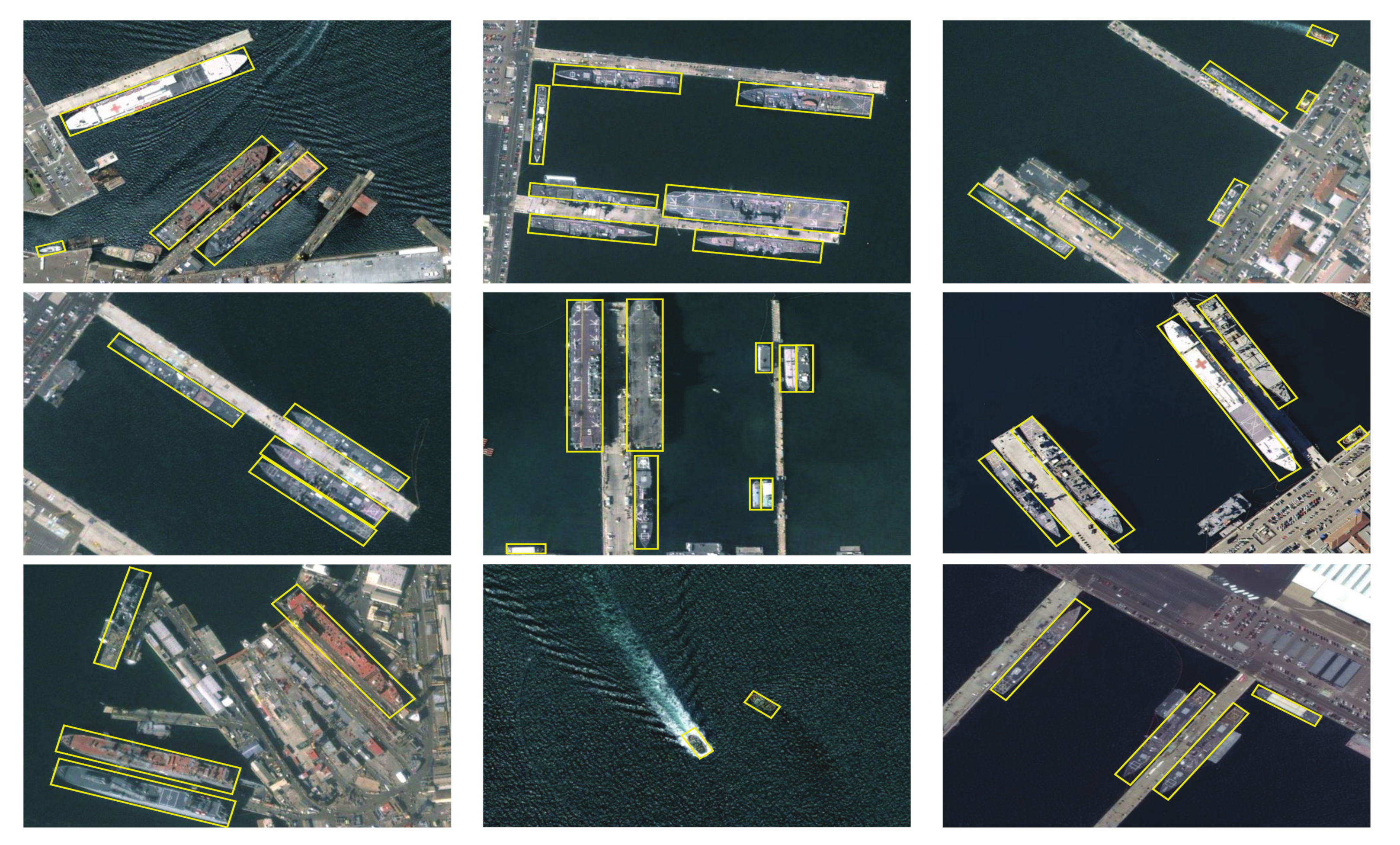
To demonstrate the superiority of our method, we also evaluated the RIE on the HRSC2016 ship dataset and compared the RIE with sixteen other oriented object detectors, as shown in Table 3. BL2 [23], RC1, and RC2 [40] are the official baselines of the HRSC2016 dataset, achieving 69.60% AP and 75.70% AP. RRD [41] introduces an activate rotating filter (ARF) and boosts the performance to 82.89% AP. In addition to these three ship detectors, we also compared our method with six other state-of-the-art anchor-based ship detectors, which were introduced in Section 2, i.e., CNN [27], RRPN [28], PN [31], RoI Trans [30], Det [33], and A-Net [35]. It can be noticed that the RIE outperformed all of the anchor-based methods with which it was compared in terms of AP. Specifically, our method boosts the performance of ship detection from the baselines of BL2 [23] (69.60%), RC1, and RC2 [40] (75.70%) to 91.27% in terms of the AP, which indicates the remarkable performance improvement for the ship identification task. Meanwhile, compared with the state-of-the-art anchor-free methods, i.e., IENet [42], Axis Learning [43], BBAVector [50], PIoU [46], GRS-Det [20], and CBDA-Net [45], the RIE outperformed them by 16.26%, 13.12%, 2.67%, 2.07%, 1.7%, and 0.77% in terms of AP. In addition, as shown in Figure 8, the ships with a large aspect ratio and multi-scale distributions could be effectively detected, and the objects could be tightly surrounded by the predicted oriented bounding boxes. These experimental results illustrate that our method can effectively capture ships in complex sea and land backgrounds.
Table 3.
Comparison of the results of accuracy and parameters on the HRSC2016 dataset.

Figure 8.
Visualization of the detection results of our method on the HRSC2016 dataset.
4.6. Accuracy–Speed Trade-Off
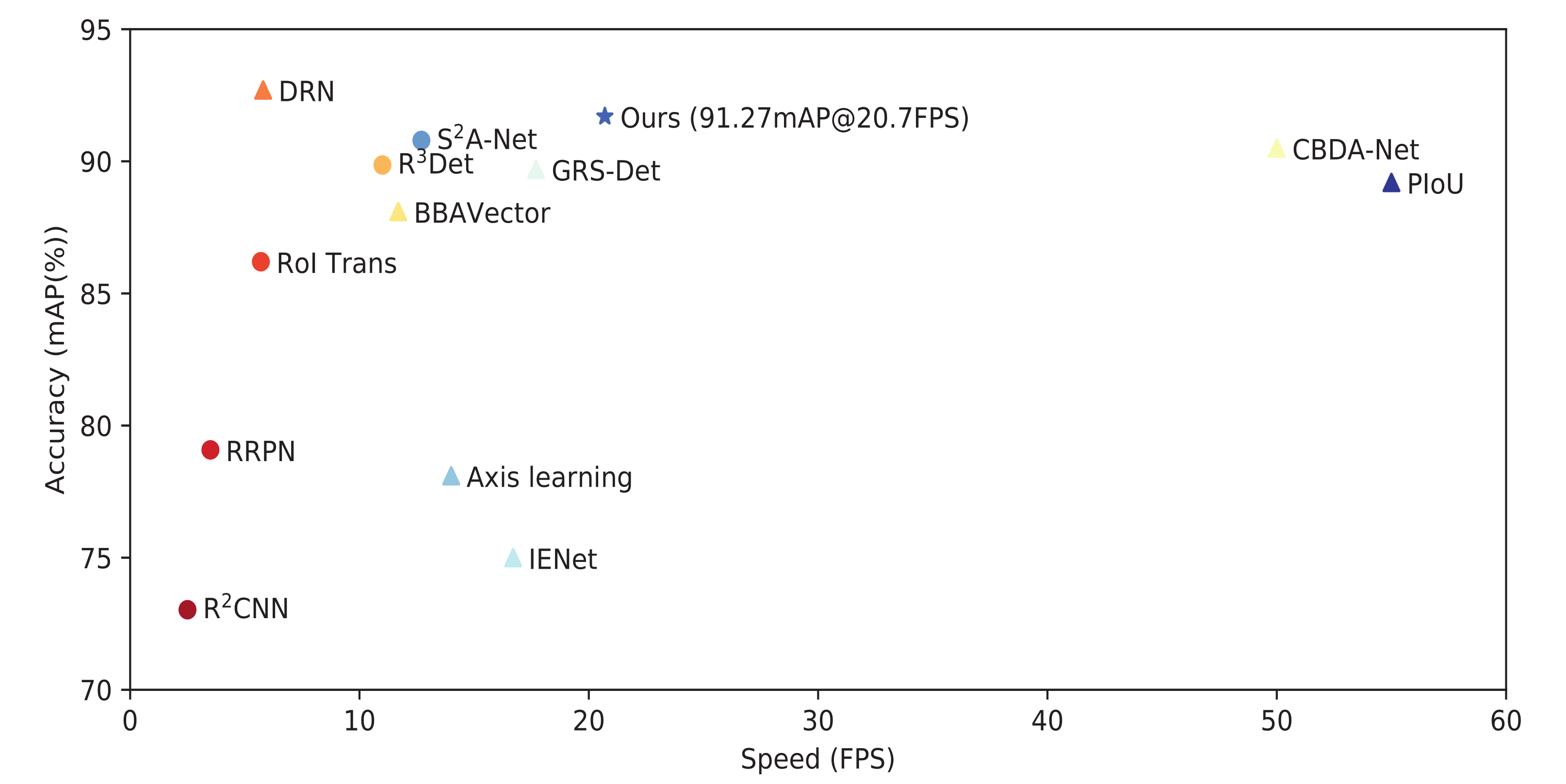
As shown in Figure 9, we plotted the results of the comparison of the accuracy and speed trade-off with our method and twelve other advanced oriented object detectors for the HRSC2016 dataset. Note that the circular sign denotes the anchor-based methods, while the triangular sign represents the anchor-free methods. The results show that the proposed method can obtain a 91.27% mAP and 20.7 FPS. For the accuracy performance, our method outperformed all of the recorded methods in Figure 9, except for the accuracy of 92.70% achieved by the DRN [47]. However, the DRN [47] under Hourglass-104 [54] runs at a slower detection speed of 5.7 FPS, while under HRGA-Net-W48, our method can run at a faster speed of 20.7 FPS. It is worth noting that our detection speed was faster than those of all other methods with which it was compared, except for the CBDA-Net [45] (50 FPS) and PIoU [46] (55 FPS), which use a more lightweight DLA-34 [61] backbone as the backbone network. At the same time, our method outperformed the two fastest detection methods, CBDA-Net [45] and PIoU [46], by 2.07% and 0.77% in terms of AP. Therefore, this confirms that our method can achieve an excellent accuracy–speed trade-off, which boosts its practical value.

Figure 9.
Accuracy versus speed on the HRSC2016 dataset.
4.7. Ablation Study
We implemented an ablation study in terms of the GAM and ewoLoss on the HRSC2016 [57] dataset, as shown in Table 4. The RIE without the GAM and ewoLoss was adopted as the baseline in the first row of Table 4. It can be seen that the baseline only achieved 81.19% and 86.15% in terms of the F1-score and mAP, respectively. For ewoLoss, we observed 4.29% and 2.48% increases in terms of the F1-score and mAP, as shown in the second row of Table 4. Furthermore, by adding the GAM, the experimental results show a 5.53% improvement in the F1-score and a 3.75% improvement in the mAP. It should be noticed that our method achieved a salient improvement in terms of precision while maintaining a higher recall metric. That indicates that our improved backbone, HRGANet-W48, can capture more robust multi-scale features of the objects with the help of the GAM, while HAGANet-W48 filters the complex background interference and further improves the detection performance. When we added the GAM and ewoLoss at the same time, the F1-score and mAP reached 87.94% and 91.27%, which are 6.75% and 5.12% higher than the baseline. Meanwhile, as shown in Table 2, we recorded the detection results of our method on the DOTA [56] dataset both with and without ewoLoss. The results indicate that the performance of the detection of objects with large aspect ratios, such as the bridge (BR), large vehicle (LV), ship (SH), and harbor (HA), was dramatically improved by adding the ewoLoss. This indicates that the proposed ewoLoss exactly boosts the accuracy of the detection of slender oriented objects with large aspect ratios. In addition, as shown in the last column of Table 4, by adding the GAM and ewoLoss, the detection results had a maximal 4.05% improvement in the mAP. These experimental results demonstrate that the GAM and ewoLoss are both conducive to the performance of oriented object identification. When both the GAM and ewoLoss are adopted, the performance is the best.
Table 4.
Ablation study of the RIE. All of the models were implemented on the HRSC2016 and DOTA datasets.
As shown in Table 5, to further explore the impacts of different representation methods, as described in Section 3.2, we compared the RIE-based representation method with the angle-based representation method on the DOTA and HRSC2016 datasets. Meanwhile, we chose three backbone networks, i.e., ResNet-101, HRNet-W48, and HRGANet-W48, to strengthen the contrast and further prove the effectiveness of the GAM. Table 5 shows the results of the comparison between the angle-based and RIE-based representation methods. The bold part represents the increment of F1-score and mAP values. On the DOTA dataset, our RIE-based representation obtained a remarkable increase of 4.41%, 3.79%, and 4.48% in the mAP under the same implementation configuration based on the ResNet-101, HRNet-W48, and HRGANet-W48 backbone networks. At the same time, on the HRSC2016 dataset, our RIE-based representation achieved a salient improvement of 4.23%, 4.30%, and 3.80% in the mAP under the same implementation configuration based on the ResNet-101, HRNet-W48, and HRGANet-W48 backbone networks. These improvement effects under different backbone networks further prove the effectiveness and robustness of our RIE-based representation method. In addition, from Table 5, we can conclude that HRGANet-W48 with the GAM can produce more improvement for each model compared with the original HRNet-W48, which further verifies the effectiveness of the GAM.
Table 5.
Results of the comparison between the angle-based and RIE-based representation methods on the DOTA and HRSC2016 datasets based on three backbone networks.
4.8. Complexity Analysis
In our method, we designed a gated aggregation model (GAM) and ewoLoss to boost the detection accuracy. Our backbone network, HRGANet-W48, increased some additional parameters and memory compared with the original HRNet-W48, which is mainly attributed to the GAM. Therefore, as shown in Table 6, we analyzed the complexity of the GAM and presented the parameters of the GAM in detail. It can be noticed that the GAM has a total of 18,504 parameters, which spend about 0.7059 MB of memory. We can see that the lightweight and efficient GAM contributes to the performance of our method with negligible computational complexity. In addition, we also recorded the total parameters of our method and several other state-of-the-art methods, such as RRPN [28], RoI Trans [30], Det [33], -Net [33], IENet [42], BBAVector [50], and GRS-Det [20], in Table 3. Our method took only approximately 207.5 MB of memory for the parameters, which is lighter than all of the other reported methods, except for the RRPN [28] and GRS-Det [20].
Table 6.
Statistical results of the GAM parameters.
4.9. Applications and Limitations
The method proposed in this article mainly aims at the detection of objects in remote sensing images. We only evaluated the proposed method in terms of the oriented object detection task on the DOTA and HRSC2016 remote sensing image datasets. To our knowledge, oriented object detectors can also be used in oblique text detection, synthetic aperture radar (SAR) image object detection, UAV target detection, seabed pockmark detection, and so on. The application prospects of our method are very broad. We will perform some experiments on these tasks to verify the superiority of our method in the future. Meanwhile, there are still many limitations in the proposed method. First, the detection speed of our method only approaches 20 FPS, which is far from reaching the standard of real-time detection. Therefore, reducing the parameters of the model and speeding up the calculation speed are the focus of the next study. Second, from the detection results on the DOTA dataset, we can see that the detection performance of our method on some objects with inter-class similarity (e.g., BC and TC) is not satisfactory. Meanwhile, our method cannot identify targets with intra-class diversity, such as different categories of ships. The overall category discrimination ability of this model is not strong. We will utilize the attention mechanism to boost the discrimination ability of our method in future work. Third, due to cloud occlusion during remote sensing image shooting, the detection performance of our method will be greatly affected. Therefore, the removal of cloud occlusion while detecting is an important research direction.
5. Conclusions
In this article, we designed a novel anchor-free center-based oriented object detector for remote sensing imagery. The proposed method abandons the angle-based bounding box representation paradigm and uses instead a six-parameter rotated inscribed ellipse (RIE) representation method . By learning the RIE in each rectangular bounding box, we can address the boundary case and angular periodicity issues of angle-based methods. Moreover, aiming at the problems of complex backgrounds and large-scale variations, we propose a high-resolution gated aggregation network to eliminate background interference and reconcile features of different scales based on a high-resolution network (HRNet) and a gated aggregation model (GAM). In addition, an eccentricity-wise orientation loss function was designed to fix the sensitivity of the RIE’s eccentricity to the orientation loss, which prominently improves the performance in the detection of objects with large aspect ratios. We performed extensive comparisons and ablation experiments on the DOTA and HRSC2016 datasets. The experimental results prove the effectiveness of our method for oriented object detection in remote sensing images. Meanwhile, the results also demonstrate that our method can achieve an excellent accuracy and speed trade-off. In future work, we will explore more efficient backbone networks and more ingenious bounding box representation methods to boost the performance in oriented object detection in remote sensing images.
Author Contributions
Methodology, L.H.; software, C.W.; validation, L.R.; formal analysis, L.H.; investigation, S.M.; resources, L.R.; data curation, S.M.; writing—original draft preparation, X.H.; writing—review and editing, X.H.; visualization, L.R.; supervision, S.M.; project administration, C.W.; funding acquisition, L.H. All authors have read and agreed to the published version of the manuscript.
Funding
This work was supported in part by the National Natural Science Foundation of China under Grant 61701524 and in part by the China Postdoctoral Science Foundation under Grant 2019M653742 (corresponding author: L.H.).
Institutional Review Board Statement
Not applicable.
Informed Consent Statement
Not applicable.
Data Availability Statement
The data used to support the findings of this study are available from the corresponding author upon request.
Conflicts of Interest
The authors declare no conflict of interest.
References
- Kamusoko, C. Importance of remote sensing and land change modeling for urbanization studies. In Urban Development in Asia and Africa; Springer: Singapore, 2017. [Google Scholar]
- Ahmad, K.; Pogorelov, K.; Riegler, M.; Conci, N.; Halvorsen, P. Social media and satellites. Multimed. Tools Appl. 2016, 78, 2837–2875. [Google Scholar] [CrossRef]
- Tang, T.; Zhou, S.; Deng, Z.; Zou, H.; Lei, L. Vehicle detection in aerial images based on region convolutional neural networks and hard negative example mining. Sensors 2017, 17, 336. [Google Scholar] [CrossRef] [PubMed] [Green Version]
- Janowski, L.; Wroblewski, R.; Dworniczak, J.; Kolakowski, M.; Rogowska, K.; Wojcik, M.; Gajewski, J. Offshore benthic habitat mapping based on object-based image analysis and geomorphometric approach. A case study from the Slupsk Bank, Southern Baltic Sea. Sci. Total Environ. 2021, 11, 149712. [Google Scholar] [CrossRef]
- Madricardo, F.; Bassani, M.; D’Acunto, G.; Calandriello, A.; Foglini, F. New evidence of a Roman road in the Venice Lagoon (Italy) based on high resolution seafloor reconstruction. Sci. Rep. 2021, 11, 1–19. [Google Scholar]
- Li, S.; Xu, Y.L.; Zhu, M.M.; Ma, S.P.; Tang, H. Remote sensing airport detection based on End-to-End deep transferable convolutional neural networks. IEEE Trans. Geosci. Remote Sens. 2019, 16, 1640–1644. [Google Scholar] [CrossRef]
- Girshick, R. Fast r-cnn. In Proceedings of the IEEE International Conference on Computer Vision, Santiago, Chile, 7–13 December 2015; pp. 1440–1448. [Google Scholar]
- Cai, Z.; Vasconcelos, N. Cascade r-cnn: Delving into high quality object detection. In Proceedings of the IEEE Conference on Computer Vision and Pattern Recognition, Salt Lake City, UT, USA, 18–22 June 2018; pp. 6154–6162. [Google Scholar]
- Ren, S.; He, K.; Girshick, R.; Sun, J. Faster r-cnn: Towards real-time object detection with region proposal networks. IEEE Trans. Pattern Anal. Mach. Intell. 2016, 39, 1137–1149. [Google Scholar] [CrossRef] [Green Version]
- Redmon, J.; Divvala, S.; Girshick, R.; Farhadi, A. You only look once: Unified, real-time object detection. In Proceedings of the IEEE Conference on Computer Vision and Pattern Recognition, Las Vegas, NV, USA, 27–30 June 2016; pp. 779–788. [Google Scholar]
- Liu, W.; Anguelov, D.; Erhan, D.; Szegedy, C.; Reed, S.; Fu, C.; Berg, A.C. Ssd: Single shot multibox detector. In Proceedings of the European Conference on Computer Vision (ECCV), Amsterdam, The Netherlands, 11–14 October 2016; pp. 21–37. [Google Scholar]
- Lin, T.Y.; Goyal, P.; Girshick, R.; He, K.; Dollár, P. Focal loss for dense object detection. In Proceedings of the IEEE International Conference on Computer Vision, Venice, Italy, 22–29 October 2017; pp. 2980–2988. [Google Scholar]
- Law, H.; Deng, J. Cornernet: Detecting objects as paired keypoints. In Proceedings of the European Conference on Computer Vision (ECCV), Munich, Germany, 8–14 September 2018; pp. 734–750. [Google Scholar]
- Duan, K.; Bai, S.; Xie, L.; Qi, H.; Huang, Q.; Tian, Q. Centernet: Keypoint triplets for object detection. In Proceedings of the IEEE International Conference on Computer Vision, Seoul, Korea, 27–28 October 2019; pp. 6569–6578. [Google Scholar]
- Zhou, X.Y.; Zhuo, J.C.; Krahenbuhl, P. Bottom-up object detection by grouping extreme and center points. In Proceedings of the IEEE Conference on Computer Vision and Pattern Recognition, Long Beach, CA, USA, 16–20 June 2019; pp. 850–859. [Google Scholar]
- Huang, L.; Yang, Y.; Deng, Y.; Yu, Y. Densebox: Unifying landmark localization with end to end object detection. arXiv 2015, arXiv:1509.04874. [Google Scholar]
- Kong, T.; Sun, F.; Liu, H.; Jiang, Y.; Li, L.; Shi, J. Foveabox: Beyound anchor-based object detection. IEEE Trans. Image Process. 2020, 29, 7389–7398. [Google Scholar] [CrossRef]
- Tian, Z.; Shen, C.; Chen, H.; He, T. Fcos: Fully convolutional one-stage object detection. In Proceedings of the IEEE International Conference on Computer Vision, Thessaloniki, Greece, 23–25 September 2019; pp. 9627–9636. [Google Scholar]
- Zhou, L.; Wei, H.; Li, H.; Zhao, W.; Zhang, Y.; Zhang, Y. Arbitrary-Oriented Object Detection in Remote Sensing Images Based on Polar Coordinates. IEEE Access 2020, 8, 223373–223384. [Google Scholar] [CrossRef]
- Zhang, X.; Wang, G.; Zhu, P.; Zhang, T.; Li, C.; Jiao, L. GRS-Det: An Anchor-Free Rotation Ship Detector Based on Gaussian-Mask in Remote Sensing Images. IEEE Trans. Geosci. Remote Sens. 2020, 59, 3518–3531. [Google Scholar] [CrossRef]
- Shi, F.; Zhang, T.; Zhang, T. Orientation-Aware Vehicle Detection in Aerial Images via an Anchor-Free Object Detection Approach. IEEE Trans. Geosci. Remote Sens. 2020, 59, 5221–5233. [Google Scholar] [CrossRef]
- Yang, X.; Yan, J. Arbitrary-Oriented Object Detection with Circular Smooth Label. In Proceedings of the 16th European Conference on Computer Vision (ECCV), Glasgow, UK, 23–28 August 2020; pp. 677–694. [Google Scholar]
- Liu, Z.; Hu, J.; Weng, L.; Yang, Y. Rotated region based CNN for ship detection. In Proceedings of the 2017 IEEE International Conference on Image Processing (ICIP), Beijing, China, 17–20 September 2017; pp. 900–904. [Google Scholar]
- Cheng, G.; Zhou, P.; Han, J. Learning Rotation-Invariant Convolutional Neural Networks for Object Detection in VHR Optical Remote Sensing Images. IEEE Trans. Geosci. Remote Sens. 2016, 54, 7405–7415. [Google Scholar] [CrossRef]
- Cheng, G.; Han, J.; Zhou, P.; Xu, D. Learning Rotation-Invariant and Fisher Discriminative Convolutional Neural Networks for Object Detection. IEEE Trans. Geosci. Remote Sens. 2019, 28, 265–278. [Google Scholar] [CrossRef] [PubMed]
- Yang, X.; Sun, H.; Fu, K.; Yang, J.; Sun, X.; Yan, M.; Guo, Z. Automatic Ship Detection in Remote Sensing Images from Google Earth of Complex Scenes Based on Multiscale Rotation Dense Feature Pyramid Networks. Remote Sens. 2018, 10, 132. [Google Scholar] [CrossRef] [Green Version]
- Jiang, Y.; Zhu, X.; Wang, X.; Yang, S.; Li, W.; Wang, H.; Fu, P.; Luo, Z. R2cnn: Rotational region cnn for orientation robust scene text detection. arXiv 2017, arXiv:1706.09579. [Google Scholar]
- Ma, J.; Shao, W.; Ye, H.; Wang, L.; Wang, H.; Zheng, Y.; Xue, X. Arbitrary-oriented scene text detection via rotation proposals. IEEE Trans. Multimed. 2018, 20, 3111–3122. [Google Scholar] [CrossRef] [Green Version]
- Azimi, S.M.; Vig, E.; Bahmanyar, R. Towards multi-class object detection in unconstrained remote sensing imagery. In Proceedings of the Asian Conference on Computer Vision, Perth, WA, Australia, 2–6 December 2018; Springer: Berlin/Heidelberg, Germany, 2018; pp. 150–165. [Google Scholar]
- Ding, J.; Xue, N.; Long, Y.; Xia, G.S.; Lu, Q. Learning RoI transformer for oriented object detection in aerial images. In Proceedings of the IEEE Conference on Computer Vision and Pattern Recognition, Long Beach, CA, USA, 16–20 June 2019; pp. 2849–2858. [Google Scholar]
- Zhang, Z.; Guo, W.; Zhu, S.; Yu, W. Toward arbitrarily oriented ship detection with rotated region proposal and discrimination networks. IEEE Geosci. Remote Sens. Lett. 2018, 15, 1745–1749. [Google Scholar] [CrossRef]
- Zhang, G.; Lu, S.; Zhang, W. Cad-net: A context-aware detection network for objects in remote sensing imagery. IEEE Trans. Geosci. Remote Sens. 2019, 57, 10015–10024. [Google Scholar] [CrossRef] [Green Version]
- Yang, X.; Liu, Q.; Yan, J.; Li, A.; Zhang, Z.; Yu, G. R3det: Refined single-stage detector with feature refinement for rotating object. arXiv 2019, arXiv:1908.05612. [Google Scholar]
- Yang, X.; Yang, J.; Yan, J.; Zhang, Y.; Zhang, T.; Guo, Z.; Sun, X.; Fu, K. Scrdet: Towards more robust detection for small, cluttered and rotated objects. In Proceedings of the IEEE International Conference on Computer Vision, Thessaloniki, Greece, 23–25 September 2019; pp. 8232–8241. [Google Scholar]
- Han, J.; Ding, J.; Li, J.; Xia, G.S. Align Deep Features for Oriented Object Detection. IEEE Trans. Geosci. Remote Sens. 2020. [Google Scholar] [CrossRef]
- Xu, Y.; Fu, M.; Wang, Q.; Wang, Y.; Chen, K.; Xia, G.S.; Bai, X. Gliding vertex on the horizontal bounding box for multi-oriented object detection. IEEE Trans. Pattern Anal. Mach. Intell. 2020, 43, 1452–1459. [Google Scholar] [CrossRef] [Green Version]
- Zhu, Y.; Du, J.; Wu, X. Adaptive Period Embedding for Representing Oriented Objects in Aerial Images. IEEE Trans. Geosci. Remote Sens. 2020, 58, 7247–7257. [Google Scholar] [CrossRef] [Green Version]
- Yang, X.; Hou, L.; Zhou, Y. Dense label encoding for boundary discontinuity free rotation detection. In Proceedings of the IEEE Conference on Computer Vision and Pattern Recognition, Las Vegas, NV, USA, 19–25 June 2016; pp. 15819–15829. [Google Scholar]
- Wu, Q.; Xiang, W.; Tang, R.; Zhu, J. Bounding Box Projection for Regression Uncertainty in Oriented Object Detection. IEEE Access 2021, 9, 58768–58779. [Google Scholar] [CrossRef]
- Liu, Z.; Yuan, L.; Weng, L.; Yang, Y. A high resolution optical satellite image dataset for ship recognition and some new baselines. In Proceedings of the International Conference on Pattern Recognition Applications and Methods, Porto, Portugal, 24–26 February 2017; Volume 2, pp. 324–331. [Google Scholar]
- Liao, M.; Zhu, Z.; Shi, B.; Xia, G.S.; Bai, X. Rotation-Sensitive Regression for Oriented Scene Text Detection. In Proceedings of the IEEE Conference on Computer Vision and Pattern Recognition (CVPR), Salt Lake City, UT, USA, 18–22 June 2018. [Google Scholar]
- Lin, Y.; Feng, P.; Guan, J. Ienet: Interacting embranchment one stage anchor free detector for orientation aerial object detection. arXiv 2019, arXiv:1912.00969. [Google Scholar]
- Xiao, Z.; Qian, L.; Shao, W.; Tan, X.; Wang, K. Axis Learning for Orientated Objects Detection in Aerial Images. Remote Sens. 2020, 12, 908. [Google Scholar] [CrossRef] [Green Version]
- Chen, J.; Xie, F.; Lu, Y.; Jiang, Z. Finding Arbitrary-Oriented Ships From Remote Sensing Images Using Corner Detection. IEEE Geosci. Remote Sens. Lett. 2019, 17, 1712–1716. [Google Scholar] [CrossRef]
- Liu, S.; Zhang, L.; Lu, H.; He, Y. Center-Boundary Dual Attention for Oriented Object Detection in Remote Sensing Images. IEEE Trans. Geosci. Remote Sens. 2021. [Google Scholar] [CrossRef]
- Chen, Z.; Chen, K.; Lin, W.; See, J.; Yu, H.; Ke, Y.; Yang, C. Piou loss: Towards accurate oriented object detection in complex environments. In Proceedings of the European Conference on Computer Vision (ECCV), Glasgow, UK, 23–28 August 2020; pp. 195–211. [Google Scholar]
- Pan, X.; Ren, Y.; Sheng, K.; Dong, W.; Yuan, H.; Guo, X.; Xu, C. Dynamic refinement network for oriented and densely packed object detection. In Proceedings of the IEEE Conference on Computer Vision and Pattern Recognition, Seattle, WA, USA, 14–19 June 2020; pp. 11207–11216. [Google Scholar]
- Wei, H.; Zhang, Y.; Chang, Z.; Li, H.; Wang, H.; Sun, X. Oriented objects as pairs of middle lines. ISPRS J. Photogramm. Remote Sens. 2020, 169, 268–279. [Google Scholar] [CrossRef]
- Wei, H.; Zhang, Y.; Wang, B.; Yang, Y.; Li, H.; Wang, H. X-LineNet: Detecting Aircraft in Remote Sensing Images by a Pair of Intersecting Line Segments. IEEE Trans. Geosci. Remote Sens. 2021, 59, 1645–1659. [Google Scholar] [CrossRef]
- Yi, J.; Wu, P.; Liu, B.; Huang, Q.; Qu, H.; Metaxas, D. Oriented Object Detection in Aerial Images with Box Boundary-Aware Vectors. In Proceedings of the IEEE/CVF Winter Conference on Applications of Computer Vision, Snowmass Village, CO, USA, 1–5 March 2020; pp. 2150–2159. [Google Scholar]
- Wang, J. Deep High-Resolution Representation Learning for Visual Recognition. IEEE Trans. Pattern Anal. Mach. Intell. 2020, 43, 3349–3364. [Google Scholar] [CrossRef] [Green Version]
- Simonyan, K.; Zisserman, A. Very deep convolutional networks for large-scale image recognition. In Proceedings of the International Conference on Learning Representations, San Diego, CA, USA, 7–9 May 2015; pp. 1–14. [Google Scholar]
- He, K.; Zhang, X.; Ren, S.; Sun, J. Deep residual learning for image recognition. In Proceedings of the IEEE Conference on Computer Vision and Pattern Recognition, Las Vegas, NV, USA, 27–30 June 2016; pp. 770–778. [Google Scholar]
- Newell, A.; Yang, K.; Deng, J. Stacked hourglass networks for human pose estimation. In Proceedings of the European Conference on Computer Vision (ECCV), Amsterdam, The Netherlands, 8–16 October 2016; pp. 483–499. [Google Scholar]
- Kendall, A.; Gal, Y.; Cipolla, R. Multi-task learning using uncertainty to weigh losses for scene geometry and semantics. In Proceedings of the IEEE Conference on Computer Vision and Pattern Recognition, Salt Lake City, UT, USA, 18–22 June 2018; pp. 7482–7491. [Google Scholar]
- Xia, G.; Bai, X.; Ding, J.; Zhu, Z.; Belongie, S.; Luo, J.; Datcu, M.; Pelillo, M.; Zhang, L. DOTA: A large-scale dataset for object detection in aerial images. In Proceedings of the IEEE Conference on Computer Vision and Pattern Recognition, Salt Lake City, UT, USA, 18–22 June 2018; pp. 3974–3983. [Google Scholar]
- Liu, Z.; Wang, H.; Weng, L.; Yang, Y. Ship rotated bounding box space for ship extraction from high-resolution optical satellite images with complex backgrounds. IEEE Geosci. Remote Sens. Lett. 2016, 13, 1074–1078. [Google Scholar] [CrossRef]
- Paszke, A.; Gross, S.; Massa, F.; Lerer, A.; Bradbury, J.; Chanan, G.; Killeen, T.; Lin, Z.M.; Gimelshein, N.; Antiga, L. Pytorch: An imperative style, high-performance deep learning library. Adv. Neural Inf. Process. Syst. 2019, 32, 8026–8037. [Google Scholar]
- Kingma, D.P.; Ba, J. Adam: A method for stochastic optimization. arXiv 2014, arXiv:1412.6980. [Google Scholar]
- Xie, S.; Girshick, R.; Dollár, P.; Tu, Z.; He, K. Aggregated residual transformations for deep neural networks. In Proceedings of the IEEE Conference on Computer Vision and Pattern Recognition, Honolulu, HI, USA, 21–26 July 2017; pp. 1492–1500. [Google Scholar]
- Yu, F.; Wang, D.; Shelhamer, E.; Darrell, T. Deep layer aggregation. In Proceedings of the IEEE Conference on Computer Vision and Pattern Recognition, Salt Lake City, UT, USA, 18–22 June 2018; pp. 2403–2412. [Google Scholar]
Publisher’s Note: MDPI stays neutral with regard to jurisdictional claims in published maps and institutional affiliations. |
© 2021 by the authors. Licensee MDPI, Basel, Switzerland. This article is an open access article distributed under the terms and conditions of the Creative Commons Attribution (CC BY) license (https://creativecommons.org/licenses/by/4.0/).