Abstract
Accurate semantic segmentation of 3D point clouds is a long-standing problem in remote sensing and computer vision. Due to the unstructured nature of point clouds, designing deep neural architectures for point cloud semantic segmentation is often not straightforward. In this work, we circumvent this problem by devising a technique to exploit structured neural architectures for unstructured data. In particular, we employ the popular convolutional neural network (CNN) architectures to perform semantic segmentation of LiDAR data. We propose a projection-based scheme that performs an angle-wise slicing of large 3D point clouds and transforms those slices into 2D grids. Accounting for intensity and reflectivity of the LiDAR input, the 2D grid allows us to construct a pseudo image for the point cloud slice. We enhance this image with low-level image processing techniques of normalization, histogram equalization, and decorrelation stretch to suit our ultimate object of semantic segmentation. A large number of images thus generated are used to induce an encoder-decoder CNN model that learns to compute a segmented 2D projection of the scene, which we finally back project to the 3D point cloud. In addition to a novel method, this article also makes a second major contribution of introducing the enhanced version of our large-scale public PC-Urban outdoor dataset which is captured in a civic setup with an Ouster LiDAR sensor. The updated dataset (PC-Urban_V2) provides nearly 8 billion points including over 100 million points labeled for 25 classes of interest. We provide a thorough evaluation of our technique on PC-Urban_V2 and three other public datasets.
1. Introduction
Semantic segmentation plays an important role in scene understanding. Traditionally, images have been used for this task. However, images fail to accurately encode the geometry of real-world scenes. In contrast, a LiDAR sensor captures precise coordinate information of multiple points in the scene, thereby preserving the 3D geometry. It readily provides depth information which is inherently more suitable for the task of semantic segmentation [1]. Consequently, 3D point clouds obtained from LiDAR are finding many applications in emerging technologies like remote sensing, site surveying, self-driving cars, and 3D urban environment modeling [2]. However, due to the unstructured and sparse nature of point clouds, their accurate semantic segmentation still remains an open research problem.
Most techniques for semantic segmentation of 3D point clouds focus on directly processing unstructured point clouds to train deep learning models [3,4,5]. PointNet [3] is the pioneering work in that regard. This technique shifted the focus of point cloud research to designing specialized 3D network architectures for unstructured data. Subsequently, many methods have been proposed to process 3D point clouds, such as PointNet++ [6], PointConv [7], FlowNet3D [8], and A-CNN [9]. However, these techniques do not fully exploit the local features of 3D point clouds. Additionally, our literature review shows that these methods underperform on real-world 3D point clouds as compared to synthetic data because of their sensitivity to noise. Direct point cloud processing with neural models also constrains the input size to impractical limits. For instance, the average sizes of input point clouds mentioned in [10,11,12] are 2 K–3 K, <1 K, and 4.8 K points, respectively. These input sizes are too small to be meaningful for practical applications. An additional problem with directly processing point clouds is that the resulting neural architectures must inadvertently rely on multi-layer perceptrons, which have a large memory footprint.
Compared to processing unstructured data with deep learning models, the processing of structured data has seen much more significant advances. In that regard, 2D convolutional neural networks (CNNs) lead the way. Hence, there have been attempts to leverage 2D CNNs for unstructured point clouds as well. Most of these attempts implement projection-based methods that either transform a point cloud into multi-view images [13,14,15,16,17,18] or convert a point cloud into spherical representation for processing [19,20]. Multiveiw transformation methods are sometimes sensitive to the selection of viewpoints, whereas the intermediary description of spherical transformation often suffers from discretization errors and occlusion problems.
In this work, we favor the projection-based approach and mitigate the issue of viewpoint selection. The first major contribution of this article is a novel projection-based method for semantic segmentation of 3D point clouds that capitalizes on the recent advancements of 2D CNNs (see Figure 1). In the proposed method, a point cloud is divided along the azimuth into multiple overlapping 3D slices of angle each. These slices are transformed into 2D multichannel pseudo images. Other LiDAR sensor outputs, such as intensity and reflectivity, are also considered in the image formation. We use an overlap region between two consecutive slices to account for occlusions and allow for sufficient context around every object in the scene. A comprehensive sweep of makes our method viewpoint invariant. When constructing our pseudo images, we also apply multiple low-level image processing techniques to render our data more suitable to the semantic segmentation task. These techniques include channel normalization, histogram equalization and decorrelation stretch, as shown in Figure 1. We use the images thus generated to train a U-Net like neural model. We employ a ResNet34 backbone for the architecture. The role of this model is to provide a 2D segmented map of the input samples that we can back project to the 3D space. After processing multiple pseudo images for a point cloud with 2D-CNN, we fuse their 3D projections to form a segmented point cloud.
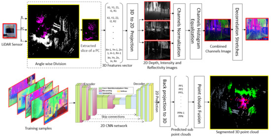
Figure 1.
Schematics of the proposed method: We perform angle-wise slicing (with overlaps) of XYZ, intensity and reflectivity channels of the LiDAR output. The slices are projected onto 2D planes where normalization and histogram equalization is applied to each channel. The channels are combined into a pseudo image. A large number of samples thus created are used to learn a U-net like 2D CNN that outputs a segmented 2D image, which we backproject to the 3D space. Point clouds resulting from the images are then fused to construct the final segmented point cloud.
In addition to a novel method for point-cloud semantic segmentation, this article also makes a second key contribution by extending our PC-Urban outdoor dataset [21]. The extension comes in the form of providing significantly more raw frames, as well as annotated frames. The proposed PC-Urban_V2 dataset is collected with an Ouster LiDAR sensor installed on an SUV which drives through the downtown of Perth city, Australia. As compared to 4 billion raw points and 20 million annotated points in [21], the updated dataset (PC-Urban_V2) contains over 8 billion raw points for more than 100 K sensor frames. The dataset has now more than ~33 K labeled instances for 25 classes comprising more than 100 million labeled data points. We use PC-Annotate tool [21] for labeling the additional points. The updated large-scale dataset will also be made public. To set up baseline results for our extended dataset with deep learning methods, we report the performance of Octree-based CNN [5], PointConv [7], PointNet++ [6], and PointNet [3] on our dataset. The results establish the presence of difficult practical scenarios in the proposed dataset. We also provide extensive experiments for our novel segmentation method by testing it on other outdoor datasets, such as semantic KITTI [22], Semantic3D [23], and Audi [24], as well as our dataset PC-Urban_V2. Overall, our proposed method outperforms recent methods in accuracy.
2. Related Work
Here, we present a brief review of the existing popular deep learning methods for point cloud semantic segmentation. We broadly divide the related literature in projection-based and point-based methods. The projection methods generally leverage transforming a point cloud into a regular representation with projection. Point-wise methods consume irregular raw 3D point clouds directly without transformation. We note that another potential category of related methods is discretization-based methods, which transform a point cloud into dense or sparse representation and feed them to 3D CNN for semantic segmentation [25,26,27,28,29,30,31,32]. These methods are generally computationally expensive. For their remote relevance to our scheme, we do not discuss methods in this category any further. Our main focus is on projection and point based methods in the text below.
2.1. Projection-Based Methods
These methods usually project a 3D point cloud onto 2D grids. Based on the underlying techniques, we can sub-categorize these methods into multi-view projection, spherical projection, and hybrid methods. The projection based methods take advantage of 2D CNNs which perform better for image semantic. segmentation. Most recent approaches include [33,34,35] which show excellent performance for 2D semantic segmentation.
Multi-view projection: Roveri et al. [14] transform a 3D point cloud into 2D depth images and then classify the depth images with well-known pre-trained 2D classification models, such as ResNet50 or VGG16. Similarly, PointPillars [13] is also a 2D CNN-based method which employs a 2D convolutional network for processing projections of point clouds. Instead of using voxels, this method uses vertical pillars. The network has three main components; pillar feature net, 2D CNN backbone, and detection head using single shot detector (SSD) [36]. The technique has low computational cost, however, the accuracy is low. In [15], a 3D point cloud is projected onto 2D planes by exploiting multiple virtual camera views. Then, pixel-wise scores are predicted on synthetic images using a multi-stream fully convolutional network. Finally, the label of each point is predicted by selecting the maximum votes for that point over various views. Likewise, in [16] several RGB and depth images of a point cloud are first generated using multiple camera positions. Then, 2D segmentation networks are deployed for pixel-wise prediction on these 2D snapshots. The predicted scores from RGB and depth images are further processed using residual correction for final prediction [18]. Based on the hypothesis that locally Euclidean surfaces have been used for point clouds sampling, another method [37] utilizes tangent convolutions for dense point cloud semantic segmentation. In this approach, first local surface geometry of each point is projected onto a virtual tangent plane. Then, tangent convolutions are applied directly on the surface geometry. This method performs well on large-scale point clouds with millions of points.
Another related technique is known as PIXOR [38] where a 2D bird’s eye view (BEV: top-to-bottom view) is exploited instead of using depth information of the scene. The method is mainly related to object detection. As it assumes that objects are on the ground, front view information is very crucial for detection. A CNN is used to detect objects, particularly in the case of autonomous cars where timely detection is a vital factor. This approach only works for the BEV and fails under other views. The large memory footprint issue in previous methods has been addressed to some extent in PointConv [7]. Both normal PointConv and memory efficient PointConv variants have been proposed for point cloud semantic segmentation by utilizing a multiplication of matrix and 2D CNN. In the case of normal 3D convolutional approaches, around 8GB memory per layer is often required, which makes the network impractical to deploy. PointConv claims to reduce the memory usage to less than 0.15 GB for each layer. Overall, the performance of multi-view segmentation methods relies rather heavily on viewpoint selection, which also results in aggravated issues in the cases of occlusions.
Spherical projection: This approach is one of the solutions for point cloud processing with deep 2D CNNs. In this projection, a point cloud is transformed onto a sphere based on azimuth and zenith angles to acquire a denser 2D grid representation. An end-to-end spherical representation based method is proposed in [20] that utilizes SqueezeNet [39] and conditional random field (CRF) for semantic segmentation of a point cloud. SqueezeSegV2 [40] is an enhanced version of the previous method to improve segmentation accuracy to resolve the domain shift issue by exploiting an unsupervised domain adaptation pipeline. RangeNet++ [19] is proposed for semantic segmentation of 3D point clouds at real-time. In this approach, labels of 2D range images are first shifted to 3D point clouds, an efficient GPU-enabled KNN-based post-processing step is further used to mitigate the problem of discretization error and blurry outputs. Spherical projection is useful for labeling LiDAR point clouds because it retains more information than a single viewpoint. Still, this intermediary description may suffer from several problems such as occlusions and errors induced by discretization.
Hybrid methods: To better extract useful features from point clouds, some methods also use multi-modal features. We refer to these as hybrid methods. A hybrid method is presented in [41] which utilizes a joint 3D-multi-view network using both RGB features and geometric features. Similarly, a cohesive point-based framework is proposed in [42] to extract 2D textural appearance, 3D structures, and global context features from 3D point clouds. Multi-view PointNet (MVPNet) [43] also combines appearance features from 2D multi-view images and spatial geometric features in the canonical point cloud space for processing 3D point clouds.
2.2. Point-Based Methods
As opposed to projections of 3D points, these methods directly deal with unstructured point clouds. Based on the network architecture considered for the feature learning of a 3D point, these methods can be further divided into pointwise MLP methods, convolution-based, graph-based, and RNN-based methods.
Pointwise MLP methods: These methods utilize and share multi-layer perceptrons (MLPs) to extract features for each point individually and then compute a global feature using a balanced aggregation function. The first 3D point cloud semantic segmentation method is PointNet [3]. It uses mini-T-nets for the transformation of input data and features, point-based MLPs, and a max pool layer for global feature extraction. However, PointNet does not extract local features which are significant for CNNs. PointNet has been extended to PointNet++ [6] which additionally extracts local features from input data by recursively applying the PointNet. Still, it ignores local features inside each region. PointNetVLAD [1] uses PointNet for extracting local features of 3D points while VLAD aggregates local features to create a global feature vector. To consider local features of 3D point clouds, a shape context-based method (ShapeContextNet) [44] is proposed. It is an end-to-end method for point cloud semantic segmentation inspired from shape context [45]. Further examples of recent point-wise techniques for classification and semantic segmentation include [46,47,48].
The PPFNET [49] is mainly directed to address the issue of local geometry in PointNet and PointNet++. In this technique, a point cloud is divided into fragments where each fragment consists of more than three local patches. The rest of the network consists of parallel PointNets (one for each local patch) and a max-pooling layer to obtain global features. However, the main issue of PPFNET is its huge memory requirement. SO-Net [50] computes spatial distribution of a 3D point cloud by extracting hierarchical features of data. In this network, a point cloud is divided into mini point clouds. Node features are calculated through multi-layers fully connected neural network and max-pooling layers. Finally, a global feature vector is obtained by applying fully connected neural networks to all node features. 3DPointCapsNet [4] has taken inspiration from 2D capsule networks [51]. The network has two parts: 3D capsule-encoder which inputs a point cloud and generates primary point capsules after passing the input through MLP and max pool layers. While at the decoder, latent capsules are fed to various MLP replicas to get local patches. In [52], a PointSIFT module is proposed to achieve scale awareness and orientation encoding by using eight spatial orientations. In PointWeb [53], mutual interactions between various points is achieved by using fully linked web in a local region. Other MLP based methods include Shellconv [54], RandLA-Net [55,56,57,58,59].
Convolution-based methods: These techniques propose effective convolution operators for point clouds semantic segmentation. An Octree-based CNN [5] with spherical kernels is used for semantic segmentation of 3D point clouds. In this method, a 3D spherical region is divided into multiple volumetric bins. A matrix of learning features is extracted by learning weights to convolution. These kernels are applied between layers of the network. The location of each layer in the network is determined by the guided octree to perform convolution in that layer. The issue of extracting local features of a point cloud has been addressed to some extent in annularly convolutional neural networks (A-CNN) [9]. In A-CNN, farthest point sampling [60] is applied to a whole point cloud to sub-sample and extract centroids randomly. Then, local regions are created in a point cloud in the form of a ring shape surrounded by the query points so that no overlap occurs between the points. Finally, a standard CNN and max pooling are applied to concatenate features for each ring. In [61], a point-wise convolution operator has been proposed, where the nearest points are placed into kernel cells and then convolved with kernel weights. In [62], a dilated point convolution operation is proposed to accumulate dilated neighboring features, instead of the K nearest neighbors.
Graph-based methods: To determine the shapes and geometric forms in 3D point clouds, numerous graph network methods are proposed. A super point graph (SPG) based technique is proposed for large-scale point cloud segmentation [63]. The SPGs are derived by partitioning point clouds into homogeneous geometrical elements. These SPGs provide more contextual relationships between object parts which are exploited by a graph convolutional network for contextual segmentation. To refine an output of this method for semantic segmentation gated graph neural networks [64] and edge-conditioned convolutions [11] are exploited. A graph-based auto-encoder and auto-decoder are designed in FoldingNet [65] for unsupervised learning of 3D point clouds. Another graph-based method is devised by using kernel correlation and graph pooling [66]. In this method, K-nearest neighbor graph is constructed to utilize neighborhood information for kernel similarity and to conduct max-pooling for each node. In [67], a supervised framework is proposed to over-segment a point cloud into pure superpoints. PyramNet [68] exploits the graph embedding module (GEM) and pyramid attention network (PAN) to capture the local geometry in 3D point clouds. Other graph-based methods include graph attention convolution [69], and a point global context reasoning [70].
RNN-based methods: Recurrent neural networks (RNNs) are used to capture inherent context features from 3D point clouds for semantic segmentation. An example of RNN-based method for segmentation of point cloud is recurrent slice network (RSNet) [71] where unordered and unstructured point clouds are transformed into an ordered sequence of vectors which are then fed to an RNN model for prediction. In [72], the approach first transforms 3D points into multi-scale grid blocks to gain input-level context. Then, the grid level features are extracted by exploiting PointNet. These features are serially given into consolidation units (CU) or recurrent consolidation units (RCU) to attain output-level context. A lightweight local dependency modeling module is proposed in [71], which utilizes a slice pooling layer to transform unordered point feature sets into a well-ordered sequence of feature vectors. A pointwise pyramid pooling module is proposed in [73] to obtain the coarse-to-fine local features and then an RNN is applied for end-to-end learning. In another work, a dynamic aggregation network [73] is proposed, which considers both global scene complexity and local geometric features. Another example in this direction is 3DCNN-DQN-RNN [74] that is claimed to perform efficient semantic parsing of large-scale point clouds. For more details on the reviewed literature, we refer interested readers to [75].
3. Proposed Method
We propose a projection-based method for semantic segmentation of 3D point clouds, see Figure 1. Recent advances in 2D CNNs allow semantic segmentation of images with high accuracy and low computational cost. Hence, our method exploits 2D CNNs for semantic segmentation of 3D point clouds. The proposed approach is specifically targeted at real-world outdoor conditions. It first splits a point cloud angle-wise into multiple 3D slices. Then, each slice is projected onto a 2D grid, constructing a pseudo image. We leverage a surface interpolation technique to project 3D point clouds onto uniform grids. In our method, we consider projection of multiple LiDAR input channels, including intensity, reflectivity, and normal values. We apply image enhancement techniques to refine the transformed pseudo images before feeding them to the 2D CNN. After processing the projections of point cloud slices, we eventually fuse the outputs of 2D CNN for the semantic segmentation of the complete point cloud. We explain the proposed method in a step-by-step manner below.
3.1. Constructing Pseudo Images from Point Clouds
In our technique, the complete point cloud is transformed into multiple 2D pseudo images using an angle-wise scan of the point cloud. These images are subsequently enhanced to create suitable training data for our 2D CNN model. In this subsection, we explain the conversion of point cloud to 2D images.
3.1.1. Slice Extraction
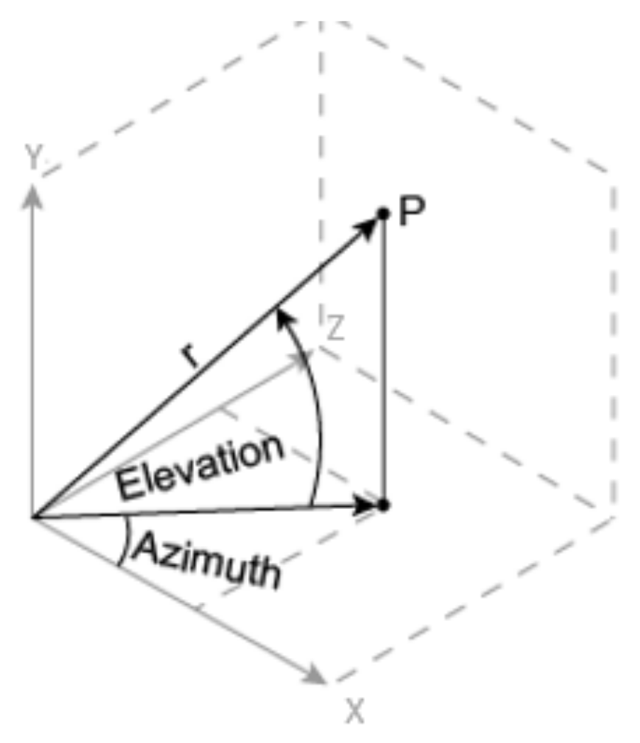
In this step, we extract slices of from the full point cloud. First X, Y, Z values of the points are converted from Cartesian coordinates to Spherical coordinates; comprising Azimuth angle, Elevation angle, and radius (r)-as shown in Figure 2.

Figure 2.
Transformation between Cartesian and Spherical coordinates.
This mapping can be reversed, which is later required in our method to obtain a back projection from 2D image to 3D point cloud. Along the Azimuth angle, points that lie inside the slice are extracted to construct a single pseudo image. We have chosen this value empirically based on our experiments. A larger value can make the image too large to be processed efficiently by the model, whereas smaller values shrink the image size, thereby reducing the spatial information therein. To bound the slice, we fix a threshold for the radius based on a histogram of 3D point cloud frame. Any value above the threshold indicated by the histogram is ignored. We do this because the density of a point cloud reduces drastically when the distance from the sensor is too large. At larger distances, i.e., large radii, very few points are encountered, which can be ignored for practicality. In our experiments, we empirically set the threshold to 70 m. A rotation along Y-axis is applied to the point cloud at a particular angle to extract a new slice. To rotate a point cloud, we apply a rotation matrix. The value for rotation angle depends upon how many slices we want to generate. For instance, when the rotation angle is , it will result in slices of the point cloud. We also split the corresponding intensity and reflectivity maps that correspond to the points in the slices. Below, we provide the expressions for mapping a point in the Cartesian coordinates to Spherical coordinates (first three), and then reverse mapping of Spherical coordinate points to the Cartesian coordinates (last three). Our technique uses these transformations to alter between the coordinate systems. Here, , and r are Azimuth angle, Elevation angle, and radius of the points in the Spherical coordinate system.
3.1.2. 3D to 2D Projection
Given the sparse nature of the point cloud, projection from 3D to 2D is not straight forward. We exploit interpolation to project a 3D slice onto a 2D grid while paying due attention to the LiDAR sensor specifications. The number of channels of a LiDAR sensor determines the vertical resolution of our grid. For instance, in the case of the proposed PC-Urban_V2 dataset, the Ouster LiDAR sensor has 64 vertical channels. The number of vertical channels for any sensor can be readily computed by looking at the samples acquired by that sensor. The horizontal resolution of our Ouster LiDAR is 1024 or 2048 points covering the full view. We divide our grid into 128 vertical units and 352 horizontal units to form a image. Here, the number of vertical units are chosen to be twice the vertical channels to ensure an acceptable grid resolution. The horizontal resolution is also adjusted with that of the LiDAR and rounded to be the vertical resolution. Note that the image size is custom chosen to suit our Ouster LiDAR and segmentation algorithm, and is not meant to match the input size of an existing CNN architecture. Hence, we must eventually design a custom CNN architecture for semantic segmentation (details in Section 3.3).
In our 2D grid, the radius values of the slice are assigned to the 2D grid based on nearest neighbor interpolation. The radius values correspond to the depth values of the point cloud. We also generate 2D grids of the corresponding intensity and reflectivity similar to the depth images. We use KNN search algorithm to cater for the cases where one-to-one correspondence is not possible. Interestingly, we found that depth images, intensity images, and the reflectivity images formed by our method often preserve complementary details of the scene. For instance, we show the three types of images for six different representative slices in Figure 3. It is noteworthy that despite transformation from 3D to 2D space, the images preserve visually discernible patterns. This makes the images suitable to be combined into a single comprehensive 3-channel pseudo image for processing by 2D CNNs. This is exactly what is done.
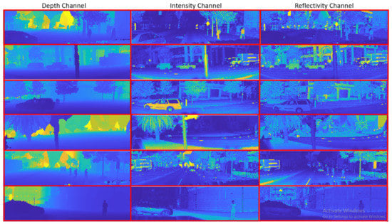
Figure 3.
Illustration of the three channels of the pseudo image constructed from 3D point cloud to 2D grid projection. (Left) Depth channel, (Middle) Intensity channel, (Right) Reflectivity channel. A point cloud slice covering view and all 64 vertical channels of the LiDAR is projected onto a grid. Pseudo colors are used for better visualization.
3.2. Image Enhancement
The next major step in preparing our pseudo images is to perform enhancement of the individual image channels constructed so far. We employ enhancement techniques such as normalization, histogram equalization and decorrelation stretch to make the images more suitable for our problem of semantic segmentation.
3.2.1. Normalization
Normalization is important to bound channel values in a meaningful range. To do so, we first estimate a threshold value for each channel based on 1000 random samples from our training data. The role of the threshold is to retain 99.9% of data by removing values that are higher than a threshold. This effectively removes outliers from the data. We have noticed that some unusual high values are often present in the intensity and reflectivity channels which are eliminated by this process. After removing the outliers, we normalize each channel by its absolute maximum value.
3.2.2. Histogram Equalization
We noted in our experiments that channels resulting from the above processing have low contrast. Thus, we employ histogram equalization to all the channels to enhance their contrast in the transformed images. We empirically found histogram equalization to benefit our ultimate objective of semantic segmentation.
3.2.3. Decorrelation Stretch
In our approach, decorrelation stretch is applied to further enhance the 2D images. The core objective of this operation is to highlight image constituents by exaggerating the color differences. We found this process to be beneficial for our multichannel LiDAR sensor images for the ultimate objective of semantic segmentation. Decorrelation stretch is a linear pixel-wise operation that accounts for actual and desired (target) image statistics. It was originally designed for multichannel images, such as RGB and multispectral tensors. In our approach, a decorrelation stretch with covariance is applied to images which uses the eigen decomposition of the band-to-band covariance matrix. This requires performing various operations sequentially, which include removing the mean value from a band, normalizing the band, rotating it in the eigenspace, applying the stretch in the eigenspace, rotating it back, rescaling and restoring the mean. Mathematically, the decorrelation stretch operation can be represented as follows:
In the above equations, a is a vector of values of a given pixel in each band of the input image A, b is the corresponding pixel in the output image B. The vector contains the mean of each band in the image, contains the desired output mean in each band. V is the orthogonal matrix of eigen vectors, denotes the diagonal matrix of eigenvalues. The band-to-band sample covariance of the image is denoted by , is the diagonal matrix comprising the sample standard deviation of each band and S is a diagonal matrix consisting of the stretch factor values. T is a linear transformation matrix which depends on , V and S. By substituting Equation (11) into Equation (7), we get the final decorrelation stretching in Equation (12).
3.3. 2D CNN Network
We extend the U-Net [76] framework and design a custom architecture to perform semantic segmentation of the converted 2D images. The proposed architecture consists of encoder and decoder parts as shown in Figure 1. Instead of using the original encoder of U-Net, we use ResNet34 architecture as the encoder in this work given the higher generalization ability of ResNet. The input image size to our network is , given as width×height×channels. The encoder part contains 2D CNN layers with a kernel size of 3 × 3, except for the first layer which has a kernel size of 7 × 7. Batch normalization, ReLU activation, and zero padding are applied before and after convolution operations at the encoder side. Stride sizes of 1 and 2 are used in the convolution either to maintain the same input size or to make the input size half in the subsequent layers. At the decoder side, up-sampling, and concatenation are applied before and after convolutions to make the output size double and increase the number of channels at the output, respectively. Moreover, batch normalization and ReLU activations are also employed after the convolution operations. The kernel size at the decoder is 1 × 1 with a stride 1. A softmax layer is used for the eventual pixel-wise prediction. There are 24.4 million trainable parameters in our network. We summarize the full architectural details of our network in Table 1.

Table 1.
The proposed encoder-decoder network architecture for semantic segmentation. ‘Y’ and ‘N’ indicate if the option is enabled or not.
3.4. Back Projection to 3D
In our approach, the prediction labels of output of the 2D CNN are in the form of a 2D grid. Each predicted value is matched to the corresponding pixel in the input multichannel image. These prediction values need to be projected back to the corresponding 3D point cloud value for the eventual semantic segmentation. We utilize the 2D depth channel values for this purpose by exploiting KNN search algorithm. The process to match X, Y, Z values of a point cloud with the predicted values is a multi-step procedure in our approach. First a complete row of a 2D depth channel is searched in the spherical coordinates of a point cloud. This returns the indices of the matched points in the point cloud. Thereafter, it is easy to extract the corresponding X, Y, Z values in the rectangular coordinate system as both rectangular and spherical coordinates share the same indexing system. In the next step, the corresponding values of a points in the rectangular domain are extracted based on the matched indices (obtained from previous step). Finally, the extracted X, Y, Z values of a point cloud are mapped to the labels in that row. Likewise, the predicted labels of all the rows are matched to the corresponding 3D point cloud values. In this way, a complete 2D grid image with corresponding labels are projected back to a sub-point cloud with predicted labels.
3.5. Fusion of 3D Sub-Point Clouds for Final Segmentation
We divide a whole point cloud into multiple sub-point clouds based on rotation angles in our approach. The CNN discussed above only processes a single sub-point cloud at a time. Hence, we need to fuse back all the predicted sub point clouds to obtain the complete segmented point cloud. At this stage, all the sub-point clouds are concatenated back based on their slice number. For instance, if four slices cover a whole point cloud with an angle of , all four slices are concatenated, disregarding the overlap between the consecutive slices. This results in redundant points along with their predictions and labels. The redundancy is resolved by randomly removing repeated points. Thus, we obtain the final complete point cloud along with its point-wise segmentation labels.
4. Proposed Dataset
The second major contribution of this article is the extension of our PC-Urban dataset [21]. In this paper, we significantly extend our dataset in terms of both unlabeled raw point clouds and annotated frames. Similar to our previous work [21], we employ the PC-Annotate tool for labeling. The data are collected in Perth, Western Australia by driving a LiDAR mounted SUV through the city. The radius of data collection region is 15 km. The collection is performed during different day and night times under varying weather conditions. Ours is a large-scale outdoor dataset that provides labels for 25 classes. It contains over 8 billion points. To put the scale of our data into perspective, Table 2 provides a summary of the popular related datasets. In the proposed PC-Urban_V2, we provide both labeled and unlabeled frames. The latter are provided to outsource annotation, as we previously provided a free public annotation tool that can be used to label raw point cloud frames [21]. Below we discuss both unlabeled and labeled frames of our dataset.
Table 2.
Popular contemporary 3D point cloud outdoor datasets for semantic segmentation task.
4.1. Unlabeled Frames
The output of LiDAR sensor is available in PCAP file format. We use Ouster Studio software to extract the raw frames. A total of 100 K raw frames containing 8 billion points were extracted from the LiDAR sensor, almost twice as much as the previous version of PC-Urban [21]. Each raw frame comprises point-wise X, Y, Z, intensity, reflectivity, ring, noise, and range values. The number of points for each frame range from 65,536 to 129,000 depending on the scene and selected horizontal resolution of the LiDAR. The same LiDAR sensor setup is used for both versions of PC-Urban except that the horizontal resolution is increased from 1024 to 2048 in the updated version. Due to its large size, the unlabeled set of PC-Urban_V2 is especially suitable for training self-supervised models. The size of unlabeled frames is more than 100 K, containing over 8 billion points.
4.2. Labeled Frames
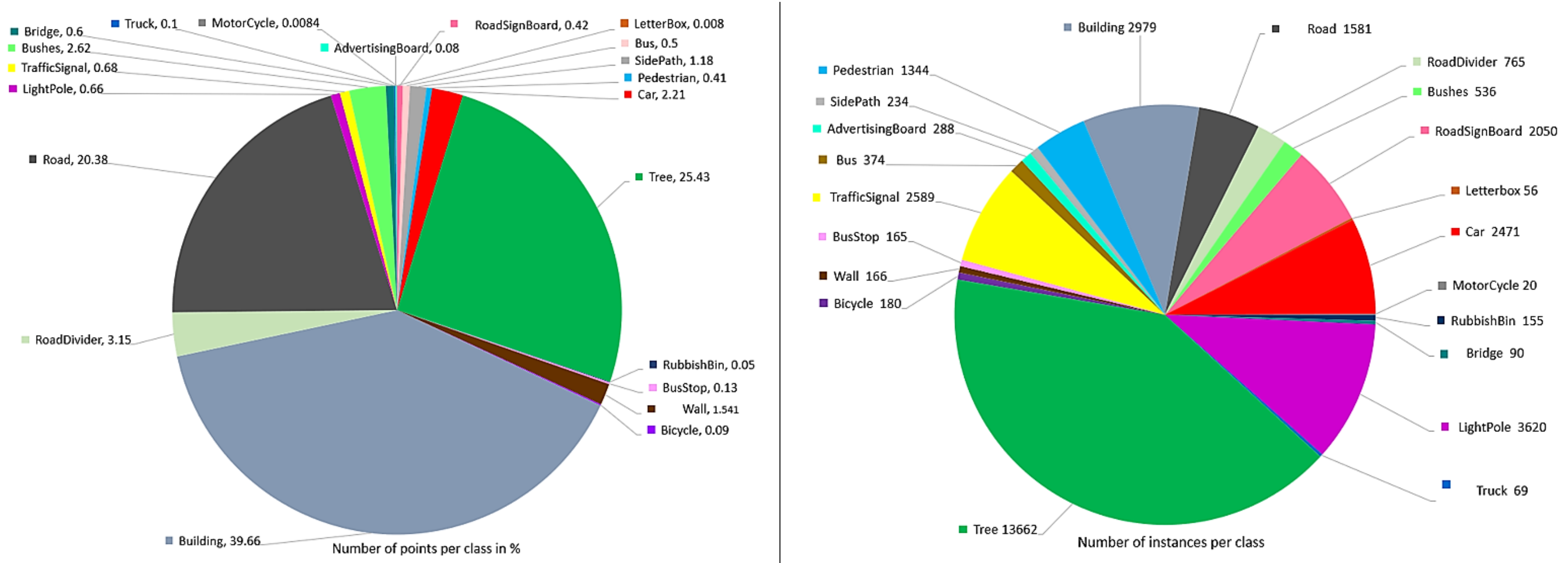
In addition to unlabeled point clouds, the dataset also provides labels for raw frames. In the dataset released with this article, there are 2000 labeled raw frames, comprising around 100 million points. These points belong to 33 K instances of objects that belong to 25 classes. In Figure 4, we show the distribution of points in the labeled raw frames for different classes of object (left), and distribution of labeled instances in the raw frames (right). Dominant classes of building, road and trees comprise 39%, 20%, and 25% points, respectively, of the total points in the dataset. Since the data are captured in an urban region where large number of trees, buildings, cars, light-poles, and traffic signals are encountered, more instances of these classes are present. The background class (not shown) carries a single instance per frame, comprising approximately 20 million points in our dataset. Labeling of 25 general outdoor classes is provided, which contain car, building, bridge, tree, road, letterbox, traffic signal, light-pole, rubbish bin, cycles, motorcycle, truck, bus, bushes, road sign board, advertising board, road divider, road lane, pedestrians, side-path, wall, bus stop, water, zebra-crossing, and background.

Figure 4.
(Left) Distribution of points per class for the raw frames of PC-Urban_V2. The distribution is provided for 100 million labeled points. For clarity, the chart excludes background points ~20 million. The number of points in millions are indicated with each class label. (Right) Distribution of the number of instances per class in the labeled raw frames.
5. Experiments
To evaluate the proposed approach, experiments are performed on multiple benchmark outdoor datasets: semantic KITTI [22], PC-Urban_V2, Semantic3D [23], and Audi [24]. Moreover, to establish the baseline on the proposed PC-Urban_V2 dataset, we test the performance of four popular deep learning methods for point cloud segmentation on our data. These methods include PointNet [3], Octree-based CNN [5], PointNet++ [6], and PointConv [7]. We select these methods based on their popularity in the literature and availability of author provided code for a fair evaluation. We also test our proposed approach on the proposed PC-Urban_V2 dataset. Semantic segmentation performance of our proposed method is compared with state-of-the-art methods. Our evaluation was performed on a machine with 2.80 GHz × 20 CPU, 128 GB RAM, and a 2080Ti GPU. Transforming a 3D point cloud into 2D pseudo images and then back projecting it, is a function of number of slices. The more slices we generate from a point cloud, the more computational cost is incurred by the process. Thus, we prefer generating more slices during the training phase for data augmentation. On the other hand, test augmentation is avoided for efficiency purpose. We organized the remaining section with respect to the datasets used.
5.1. PC-Urban_V2 Dataset
To benchmark techniques on the proposed extended PC-Urban dataset, we experiment with PointNet [3], Octree-based CNN [5], PointNet++ [6] and PointConv [7], and our proposed method.
Experiment Setup: A total of 2000 annotated frames of PC-Urban_V2 dataset are used for all the considered methods. From the annotated data, we use 1500 frames (i.e., ~75%) for training and 500 frames (i.e., ~25%) for testing. For a fair comparison, all the techniques are trained for 200 epochs. We exploit the original available Tensorflow implementations for the used approaches. However, Keras is also used for our proposed method.
Setting for the proposed technique and data: The transformation from 3D to 2D explained in Section 3 is applied to the proposed dataset for our method. To generate more training data, we apply a rotation angle of and generate a total of 72 2D grid images from a single point cloud. Thus, a total of 108,000 training images are created from 1500 training point cloud frames. Recall that at inference time we only apply rotations to generate only 4 2D grid images for fast processing and hence only 2000 images are created from the 500 test point cloud frames. All 2D grid images are preprocessed as mentioned in Section 3.
Setting for other methods: We use the settings recommended by the original authors for the remaining techniques according to their requirements. For Octree-based CNN [5], Tensorflow TFrecord is used for data preparation. For PointNet [3], PointNet++ [6], and PointConv [7], our PC-Annotate tool is utilized for data preparation. For all methods, from the 1500 training point cloud frames, random 2.4 million (2,386,000 to be precise) samples were extracted for training. Similarly, from the 500 test point cloud frames, 750,000 samples were extracted for testing. The size of each sample is kept 4096 to suit the input size of the methods we have used for comparison. Each point consists of X, Y, Z, and the three normal vector values.
Results on PC-Urban_V2
Table 3 summarizes the performance of our experiments for point cloud semantic segmentation on PC-Urban_V2. The table includes results of our proposed approach and other popular techniques used for comparison. The performance is reported using the standard evaluation metrics: mean Intersection over Union (mIoU) and overall accuracy (OA). As can be seen, values for these metrics and per class accuracy for PointNet and PointNet++ are fairly low as compared to other approaches on PC-Urban_V2 dataset. This is mainly because PointNet and PointNet++ largely ignore local features in 3D point clouds. On the other hand, PointConv [7] and Octree-based CNN [5] results are more promising. However, the proposed approach outperforms all other methods by a significant margin. Our results show reasonable preservation of spatial patterns in the data by exploiting structured 2D CNNs. The performance of our approach on PC-Urban_V2 in terms of mIoU is a significant 24% better than the best performing unstructured CNN based approach [5]. Additionally, per class accuracy for most of the representative classes shown in the table is better than other methods.
Table 3.
Semantic segmentation results comparison of popular techniques with our proposed method on the proposed PC-Urban_V2 dataset. We report the mean intersection over union (mIoU) and overall accuracy (OA) in %, for comparison. Class-wise segmentation performance (IoU in %) for 17 representative classes is reported. However, the mIoU and OA are computed for all 25 classes. The first and second best results are highlighted in blue and green colors, respectively.
5.2. Semantic KITTI Dataset
We also benchmark our proposed method on one of the most popular datasets for 3D semantic segmentation, i.e., semantic KITTI outdoor dataset. This is a large dataset captured with the Velodyne HDL-64E LiDAR and provides point-wise annotations for 28 classes suitable for a variety of tasks. The dataset is different from other laser datasets in that it provides scan-wise annotations for a total of 22 annotated sequences. Annotations only for the first 10 sequences are publicly available and hence we use these for our training and testing. The results of existing methods are reported from [86] that follow the same protocol as evaluation of our method.
Experimental setup and data preparation: We use a total of 19,069 annotated frames of semantic KITTI data. Out of these, we use approximately 14 K frames (i.e., 75%) for training and 5 K frames (i.e., 25%) for testing. During training we use 5% of the training data for validation. The size of each frame varies from 90 K to 130 K points. The transformation from 3D to 2D explained in Section 3 is applied to these extracted frames. To augment training data, we apply a rotation angle of to generate 36 2D grid images from each 3D point cloud frame. During testing and inference, we apply rotations to generate only 4 2D grid images for fast processing. Pre-processing techniques mentioned in Section 3 are applied to both training and test images. We train our proposed model for 150 epochs on this dataset using the Keras and Tensorflow.
Results on Semantic KITTI Dataset
Table 4 compares the semantic segmentation results of our method with the popular recent approaches on the semantic KITTI dataset. The semantic segmentation metric of mean intersection over union (mIoU) is used again for comparison for all classes, as well as for individual representative classes of the semantic KITTI dataset. Our approach outperforms all the recent methods in terms of mIoU except RPVNet [87], S3Net [88], and Cylinder3D [89]. The performance of RPVNet [87], S3Net [88], and Cylinder3D [89] are slighter better than our approach. Our method outperformed all other approaches in terms of class-wise accuracy on six classes including bicycle, truck, other-vehicle, bicyclist, other-ground, and fence. Overall, the results of our technique are highly competitive on this dataset.
Table 4.
Semantic segmentation performance comparison of popular techniques with our method on Semantic KITTI dataset. We report the mean intersection over union (mIoU) in %. Class-wise segmentation performance comparison of our method with state-of-the-art methods for representative classes of Semantic KITTI dataset are also given. The results are in %IoU. The first and second best results are highlighted in blue and green colors, respectively.
5.3. Semantic3D Dataset
We also report comparative results on the Semantic3D outdoor dataset which contains over 4 billion labeled points. The dataset covers a wide range of urban scenes including streets, churches, railroad tracks, squares, villages, soccer fields, and castles. The performance of our approach is compared with popular recent methods for eight classes namely, man-made terrain, natural terrain, high vegetarian, low vegetarian, buildings, hardscape, scanning artifacts, and car.
Experimental setup: The pre-defined training and test sets of Semantic3D dataset are used for training and testing our method. The same train and test splits are used by all compared methods. In our case, we use 10% of the training samples for validation during training and train network for 200 epochs.
Data preparation for our method: The same transformation method explained in Section 3 is used to create 2D grid images for both training and testing. We use a much smaller rotation angle () to extract 720 2D grid images from each point cloud frame. This resulted in a total of 10,800 images from 15 annotated 3D point cloud frames for training. For testing, the rotation angle is kept the same as the previous datasets, i.e., rotation is applied to extract 4 2D grid images from each point cloud frame. Pre-processing techniques mentioned in Section 3 are also applied on both training and test images.
Results on Semantic3D
Table 5 reports the semantic segmentation results of our proposed method and popular recent approaches on the Semantic3D dataset. We report the overall accuracy (OA) and the mIoU of all nine classes including the background class for comparison, as well as the class-wise accuracy for eight classes (excluding the background class). Our approach outperformed all techniques on the mIoU metric. Note that, the compared techniques include many high performing techniques, such as WreathProdNet [98], ConvPoint [99], SPGraph [63], WOW [100], and PointConv_CE [101]. Nevertheless, our method outperformed these methods on mIoU, while also maintaining better individual class accuracy for multiple classes.
Table 5.
Semantic segmentation performance comparison of popular techniques with our method on Semantic3D. We report the mean intersection over union (mIoU) and overall accuracy (OA) in %. Class-wise segmentation performance of methods is also provided as %IoU. H-Veg, L-Veg, MM-Terrain, N-Terrain, S-Art, respectively, stand for high vegetarian, low vegetarian, man-made terrain, natural terrain, and scanning artifacts. The first and second best results are highlighted in blue and green colors, respectively.
5.4. Audi Dataset
We further test our approach on the very recently released Audi dataset [24] which provides 41,277 frames for semantic segmentation of both 3D points and 2D RGB images. This dataset was captured specifically for autonomous driving. Multiple 16 channel LiDAR sensors and RGB cameras were mounted on the roof of a car for data collection. Positions of sensors and their corresponding cameras are as follows: front center, front left, front right, side left, side right, and rear center. Each frame contains an RBG image, 2D ground-truth image and its corresponding point cloud. This dataset is mainly for 2D analysis and the point cloud data are meant to assist the 2D methods.
Experiment setup and data preparation: Out of 41,277 LiDAR frames, approximately 31 K (i.e., 75%) frames are used for training our method, whereas 10 K (i.e., 25%) are used for testing. During training, we use 5% of the training data for validation and train our model for 200 epochs. For both the transformation method explained in Section 3 is used for that purpose. Due to smaller number of channels of LiDAR in the data, the resolution of each LiDAR frame is very low. Each 3D point cloud frame comprises points in the range 7 K to 13 K. Thus, a large rotation angle is selected to divide a point cloud into less number of slices for training data augmentation. We use a rotation angle of to get two 2D grid images from each point cloud frame. Unlike the previous datasets, the test data are also processed similarly to get 2 images from each point cloud frame. In total 82.5 K 2D grid images are generated out of 41.2 K frames for both training and testing with a proportion of 3:1, respectively. Image enhancement techniques mentioned in Section 3 are then applied for both training and testing images.
Results on Audi Dataset
In Table 6, we report the semantic segmentation results of our approach on the Audi dataset. We use mIoU, OA, and recall as performance metrics. Class-wise accuracy is also reported for car, truck, pedestrian, bicycle, ego car, small vehicle, utility vehicle, and animals. This establishes the first baseline results for the Audi dataset as no other method has reported semantic segmentation results on this dataset using point clouds only. This is mainly because the point cloud resolution and density is very low in this dataset. This is also the reason we are unable to test other methods on this dataset for comparison. Nevertheless, our proposed method is still applicable on this low resolution point cloud dataset. We report the first baseline results for semantic segmentation on the Audi dataset, which is a contribution in itself. Note that the performance of our method on Audi dataset is quite low because of the very low resolution 3D point cloud frames, i.e., 16 channels as opposed to 64 channels in PC-Urban_V2 and KITTI datasets. However, from a practical standpoint, the Audi dataset is still realistic and our technique is able to provide a strong baseline for the semantic segmentation task on this dataset.
Table 6.
Semantic segmentation results of our method on Audi dataset. We report mean intersection over union (mIoU), overall accuracy (OA), recall and class-wise segmentation performance of our method for different classes of Audi dataset.
6. Conclusions
This article proposed a projection-based method for 3D point cloud semantic segmentation. The proposed technique first transforms a 3D point cloud into 2D grid images and then exploits a U-Net like 2D structured CNNs architecture for semantic segmentation. Our method has the benefit that it allows taking advantage of advances in 2D CNNs, which have matured more than their unstructured 3D counterparts. Our approach is trained and evaluated on recent popular 3D point cloud datasets, including PC-Urban_V2, Semantic KITTI, Semantic3D, and Audi. The second major contribution of this work is the extension of PC-Urban dataset in terms of labeled and unlabeled data. We plan to extend the proposed PC-Urban_V2 dataset in the future in terms of both labels and raw data. We also provided baseline results for point cloud semantic segmentation on our dataset using recent popular deep learning techniques along with comparison to the proposed method. These results establish that the proposed dataset provides more challenging scenarios. At the same time, strong results provided by our method establish the effectiveness of our approach.
Author Contributions
Conceptualization, M.I., N.A. and A.M.; methodology, M.I., N.A., K.U. and A.M.; software, M.I.; validation, M.I., N.A., K.U. and A.M.; formal analysis, M.I. and N.A.; investigation, M.I., N.A., K.U. and A.M.; resources, A.M.; data curation, M.I., N.A., A.M.; writing—original draft preparation, M.I.; writing—review and editing, N.A., K.U., A.M.; visualization, M.I. and N.A.; supervision, N.A. and A.M.; project administration, A.M.; funding acquisition, N.A. and A.M. All authors have read and agreed to the published version of the manuscript.
Funding
This research was supported by the Australian Research Council Discovery Grant DP190102443. Naveed Akhtar is the recipient of an Office of National Intelligence (ONI) National Intelligence Postdoctoral Grant funded by the Australian Government.
Conflicts of Interest
The authors declare no conflict of interest.
References
- Angelina Uy, M.; Hee Lee, G. PointNetVLAD: Deep point cloud based retrieval for large-scale place recognition. In Proceedings of the IEEE Conference on CVPR, Salt Lake City, UT, USA, 18–23 June 2018; pp. 4470–4479. [Google Scholar]
- Hammoudi, K.; Dornaika, F.; Soheilian, B.; Paparoditis, N. Extracting wire-frame models of street facades from 3D point clouds and the corresponding cadastral map. IAPRS 2010, 38, 91–96. [Google Scholar]
- Qi, C.R.; Su, H.; Mo, K.; Guibas, L.J. Pointnet: Deep learning on point sets for 3d classification and segmentation. In Proceedings of the IEEE Conference on Computer Vision and Pattern Recognition, Honolulu, HI, USA, 21–26 July 2017; pp. 652–660. [Google Scholar]
- Zhao, Y.; Birdal, T.; Deng, H.; Tombari, F. 3D Point Capsule Networks. In Proceedings of the IEEE/CVF Conference on Computer Vision and Pattern Recognition, Long Beach, CA, USA, 15–20 June 2019; pp. 1009–1018. [Google Scholar]
- Lei, H.; Akhtar, N.; Mian, A. Octree Guided CNN With Spherical Kernels for 3D Point Clouds. In Proceedings of the IEEE/CVF Conference on Computer Vision and Pattern Recognition, Long Beach, CA, USA, 15–20 June 2019. [Google Scholar]
- Qi, C.R.; Yi, L.; Su, H.; Guibas, L.J. Pointnet++: Deep hierarchical feature learning on point sets in a metric space. In Proceedings of the Advances in Neural Information Processing Systems, Long Beach, CA, USA, 4–7 December 2017; pp. 5099–5108. [Google Scholar]
- Wu, W.; Qi, Z.; Fuxin, L. PointConv: Deep Convolutional Networks on 3D Point Clouds. In Proceedings of the IEEE/CVF Conference on Computer Vision and Pattern Recognition (CVPR), Long Beach, CA, USA, 15–20 June 2019; pp. 9621–9630. [Google Scholar]
- Liu, X.; Qi, C.R.; Guibas, L.J. Flownet3d: Learning scene flow in 3d point clouds. In Proceedings of the IEEE/CVF Conference on Computer Vision and Pattern Recognition, Long Beach, CA, USA, 15–20 June 2019; pp. 529–537. [Google Scholar]
- Komarichev, A.; Zhong, Z.; Hua, J. A-CNN: Annularly Convolutional Neural Networks on Point Clouds. In Proceedings of the IEEE/CVF Conference on Computer Vision and Pattern Recognition, Long Beach, CA, USA, 15–20 June 2019; pp. 7421–7430. [Google Scholar]
- Yi, L.; Su, H.; Guo, X.; Guibas, L.J. Syncspeccnn: Synchronized spectral cnn for 3d shape segmentation. In Proceedings of the IEEE/CVF Conference on Computer Vision and Pattern Recognition, Honolulu, HI, USA, 21–26 July 2017; pp. 2282–2290. [Google Scholar]
- Simonovsky, M.; Komodakis, N. Dynamic edge-conditioned filters in convolutional neural networks on graphs. In Proceedings of the IEEE Conference on Computer Vision and Pattern Recognition, Honolulu, HI, USA, 21–26 July 2017; pp. 3693–3702. [Google Scholar]
- Qi, X.; Liao, R.; Jia, J.; Fidler, S.; Urtasun, R. 3d graph neural networks for rgbd semantic segmentation. In Proceedings of the IEEE International Conference on Computer Vision, Honolulu, HI, USA, 21–26 July 2017; pp. 5199–5208. [Google Scholar]
- Lang, A.H.; Vora, S.; Caesar, H.; Zhou, L.; Yang, J.; Beijbom, O. PointPillars: Fast encoders for object detection from point clouds. In Proceedings of the IEEE/CVF Conference on Computer Vision and Pattern Recognition, Long Beach, CA, USA, 15–20 June 2019; pp. 12697–12705. [Google Scholar]
- Roveri, R.; Rahmann, L.; Oztireli, C.; Gross, M. A network architecture for point cloud classification via automatic depth images generation. In Proceedings of the IEEE Conference on Computer Vision and Pattern Recognition, Salt Lake City, UT, USA, 18–23 June 2018; pp. 4176–4184. [Google Scholar]
- Lawin, F.J.; Danelljan, M.; Tosteberg, P.; Bhat, G.; Khan, F.S.; Felsberg, M. Deep projective 3D semantic segmentation. In Proceedings of the International Conference on Computer Analysis of Images and Patterns, Ystad, Sweden, 22–24 August 2017; Springer: Cham, Switerland, 2017; pp. 95–107. [Google Scholar]
- Boulch, A.; Le Saux, B.; Audebert, N. Unstructured Point Cloud Semantic Labeling Using Deep Segmentation Networks. 3DOR Eurographics 2017, 2, 7. [Google Scholar] [CrossRef]
- Armeni, I.; Sener, O.; Zamir, A.R.; Jiang, H.; Brilakis, I.; Fischer, M.; Savarese, S. 3d semantic parsing of large-scale indoor spaces. In Proceedings of the IEEE Conference on Computer Vision and Pattern Recognition, Las Vegas, NV, USA, 27–30 June 2016; pp. 1534–1543. [Google Scholar]
- Audebert, N.; Le Saux, B.; Lefèvre, S. Semantic segmentation of earth observation data using multimodal and multi-scale deep networks. In Proceedings of the Asian Conference on Computer Vision, Taipei, Taiwan, 20–24 November 2016; Springer: Cham, Switerland, 2016; pp. 180–196. [Google Scholar]
- Milioto, A.; Vizzo, I.; Behley, J.; Stachniss, C. Rangenet++: Fast and accurate lidar semantic segmentation. In Proceedings of the 2019 IEEE/RSJ International Conference on Intelligent Robots and Systems (IROS), The Venetian Macao, Macau, China, 4–8 November 2019; pp. 4213–4220. [Google Scholar]
- Wu, B.; Wan, A.; Yue, X.; Keutzer, K. Squeezeseg: Convolutional neural nets with recurrent crf for real-time road-object segmentation from 3d lidar point cloud. In Proceedings of the 2018 IEEE International Conference on Robotics and Automation (ICRA), Brisbane, Australia, 21–26 May 2018; pp. 1887–1893. [Google Scholar]
- Ibrahim, M.; Akhtar, N.; Wise, M.; Mian, A. Annotation Tool and Urban Dataset for 3D Point Cloud Semantic Segmentation. IEEE Access 2021, 9, 35984–35996. [Google Scholar] [CrossRef]
- Behley, J.; Garbade, M.; Milioto, A.; Quenzel, J.; Behnke, S.; Stachniss, C.; Gall, J. SemanticKITTI: A Dataset for Semantic Scene Understanding of LiDAR Sequences. In Proceedings of the IEEE/CVF International Conference on Computer Vision (ICCV), Seoul, Korea, 27 October–3 November 2019. [Google Scholar]
- Hackel, T.; Savinov, N.; Ladicky, L.; Wegner, J.D.; Schindler, K.; Pollefeys, M. Semantic3d. net: A new large-scale point cloud classification benchmark. arXiv 2017, arXiv:1704.03847. [Google Scholar]
- Geyer, J.; Kassahun, Y.; Mahmudi, M.; Ricou, X.; Durgesh, R.; Chung, A.S.; Hauswald, L.; Pham, V.H.; Mühlegg, M.; Dorn, S.; et al. A2D2: AEV Autonomous Driving Dataset. Available online: http://www.a2d2.audi (accessed on 14 April 2020).
- Graham, B.; Engelcke, M.; Van Der Maaten, L. 3d semantic segmentation with submanifold sparse convolutional networks. In Proceedings of the IEEE Conference on Computer Vision and Pattern Recognition, Salt Lake City, UT, USA, 18–23 June 2018; pp. 9224–9232. [Google Scholar]
- Huang, J.; You, S. Point cloud labeling using 3d convolutional neural network. In Proceedings of the 2016 23rd International Conference on Pattern Recognition (ICPR), Cancun, Mexico, 4–8 December 2016; pp. 2670–2675. [Google Scholar]
- Dai, A.; Ritchie, D.; Bokeloh, M.; Reed, S.; Sturm, J.; Nießner, M. Scancomplete: Large-scale scene completion and semantic segmentation for 3d scans. In Proceedings of the IEEE Conference on Computer Vision and Pattern Recognition, Salt Lake City, UT, USA, 18–23 June 2018; pp. 4578–4587. [Google Scholar]
- Rethage, D.; Wald, J.; Sturm, J.; Navab, N.; Tombari, F. Fully-convolutional point networks for large-scale point clouds. In Proceedings of the European Conference on Computer Vision (ECCV), Munich, Germany, 8–14 September 2018; pp. 596–611. [Google Scholar]
- Meng, H.Y.; Gao, L.; Lai, Y.K.; Manocha, D. Vv-net: Voxel vae net with group convolutions for point cloud segmentation. In Proceedings of the IEEE/CVF International Conference on Computer Vision, Seoul, Korea, 27 October–3 November 2019; pp. 8500–8508. [Google Scholar]
- Zhou, Y.; Tuzel, O. Voxelnet: End-to-end learning for point cloud based 3d object detection. In Proceedings of the IEEE Conference on Computer Vision and Pattern Recognition, Salt Lake City, UT, USA, 18–23 June 2018; pp. 4490–4499. [Google Scholar]
- Ren, S.; He, K.; Girshick, R.; Sun, J. Faster r-cnn: Towards real-time object detection with region proposal networks. In Proceedings of the Advances in Neural Information Processing Systems, Montreal, QC, Canada, 7–10 December 2015; pp. 91–99. [Google Scholar]
- Wu, Z.; Song, S.; Khosla, A.; Yu, F.; Zhang, L.; Tang, X.; Xiao, J. 3d shapenets: A deep representation for volumetric shapes. In Proceedings of the IEEE Conference on Computer Vision and Pattern Recognition, Boston, MA, USA, 7–12 June 2015; pp. 1912–1920. [Google Scholar]
- Takikawa, T.; Acuna, D.; Jampani, V.; Fidler, S. Gated-scnn: Gated shape cnns for semantic segmentation. In Proceedings of the IEEE/CVF International Conference on Computer Vision, Seoul, Korea, 27 October–3 November 2019; pp. 5229–5238. [Google Scholar]
- Min, L.; Cui, Q.; Jin, Z.; Zeng, T. Inhomogeneous image segmentation based on local constant and global smoothness priors. Digit. Signal Process. 2021, 111, 102989. [Google Scholar] [CrossRef]
- Fang, Y.; Zeng, T. Learning deep edge prior for image denoising. Comput. Vis. Image Underst. 2020, 200, 103044. [Google Scholar] [CrossRef]
- Liu, W.; Anguelov, D.; Erhan, D.; Szegedy, C.; Reed, S.; Fu, C.Y.; Berg, A.C. Ssd: Single shot multibox detector. In Proceedings of the European Conference on Computer Vision, Amsterdam, The Netherlands, 8–16 October 2016; pp. 21–37. [Google Scholar]
- Tatarchenko, M.; Park, J.; Koltun, V.; Zhou, Q.Y. Tangent convolutions for dense prediction in 3d. In Proceedings of the IEEE Conference on Computer Vision and Pattern Recognition, Salt Lake City, UT, USA, 18–23 June 2018; pp. 3887–3896. [Google Scholar]
- Yang, B.; Luo, W.; Urtasun, R. Pixor: Real-time 3d object detection from point clouds. In Proceedings of the IEEE Conference on Computer Vision and Pattern Recognition, Salt Lake City, UT, USA, 18–23 June 2018; pp. 7652–7660. [Google Scholar]
- Iandola, F.N.; Han, S.; Moskewicz, M.W.; Ashraf, K.; Dally, W.J.; Keutzer, K. SqueezeNet: AlexNet-level accuracy with 50x fewer parameters and <0.5 MB model size. arXiv 2016, arXiv:1602.07360. [Google Scholar]
- Wu, B.; Zhou, X.; Zhao, S.; Yue, X.; Keutzer, K. Squeezesegv2: Improved model structure and unsupervised domain adaptation for road-object segmentation from a lidar point cloud. In Proceedings of the 2019 International Conference on Robotics and Automation (ICRA), ICRA 2019, Montreal, QC, Canada, 20–24 May 2019; pp. 4376–4382. [Google Scholar]
- Dai, A.; Nießner, M. 3dmv: Joint 3d-multi-view prediction for 3d semantic scene segmentation. In Proceedings of the European Conference on Computer Vision (ECCV), Munich, Germany, 8–14 September 2018; pp. 452–468. [Google Scholar]
- Chiang, H.Y.; Lin, Y.L.; Liu, Y.C.; Hsu, W.H. A unified point-based framework for 3d segmentation. In Proceedings of the 2019 International Conference on 3D Vision (3DV), 3DV 2019, Québec City, QC, Canada, 16–19 September 2019; pp. 155–163. [Google Scholar]
- Jaritz, M.; Gu, J.; Su, H. Multi-view pointnet for 3d scene understanding. In Proceedings of the IEEE/CVF International Conference on Computer Vision Workshops, Seoul, Korea, 27–28 October 2019. [Google Scholar]
- Xie, S.; Liu, S.; Chen, Z.; Tu, Z. Attentional shapecontextnet for point cloud recognition. In Proceedings of the IEEE Conference on Computer Vision and Pattern Recognition, Salt Lake City, UT, USA, 18–23 June 2018; pp. 4606–4615. [Google Scholar]
- Belongie, S.; Malik, J.; Puzicha, J. Shape matching and object recognition using shape contexts. IEEE Trans. PAMI 2002, 11, 509–522. [Google Scholar] [CrossRef] [Green Version]
- Qiu, S.; Anwar, S.; Barnes, N. Geometric back-projection network for point cloud classification. IEEE Trans. Multimed. 2021. [Google Scholar] [CrossRef]
- Qiu, S.; Anwar, S.; Barnes, N. Semantic Segmentation for Real Point Cloud Scenes via Bilateral Augmentation and Adaptive Fusion. In Proceedings of the IEEE/CVF Conference on Computer Vision and Pattern Recognition, Virtual, 19–25 June 2021; pp. 1757–1767. [Google Scholar]
- Qiu, S.; Anwar, S.; Barnes, N. Dense-resolution network for point cloud classification and segmentation. In Proceedings of the IEEE/CVF Winter Conference on Applications of Computer Vision, Virtual, 5–9 January 2021; pp. 3813–3822. [Google Scholar]
- Deng, H.; Birdal, T.; Ilic, S. Ppfnet: Global context aware local features for robust 3d point matching. In Proceedings of the IEEE Conference on Computer Vision and Pattern Recognition, Salt Lake City, UT, USA, 18–23 June 2018; pp. 195–205. [Google Scholar]
- Li, J.; Chen, B.M.; Hee Lee, G. So-net: Self-organizing network for point cloud analysis. In Proceedings of the IEEE Conference on Computer Vision and Pattern Recognition, Salt Lake City, UT, USA, 18–23 June 2018; pp. 9397–9406. [Google Scholar]
- Sabour, S.; Frosst, N.; Hinton, G.E. Dynamic routing between capsules. In Proceedings of the Advances in Neural Information Processing Systems, Long Beach, CA, USA, 4–7 December 2017; pp. 3856–3866. [Google Scholar]
- Jiang, M.; Wu, Y.; Zhao, T.; Zhao, Z.; Lu, C. Pointsift: A sift-like network module for 3d point cloud semantic segmentation. arXiv 2018, arXiv:1807.00652. [Google Scholar]
- Zhao, H.; Jiang, L.; Fu, C.W.; Jia, J. Pointweb: Enhancing local neighborhood features for point cloud processing. In Proceedings of the IEEE/CVF Conference on Computer Vision and Pattern Recognition, Long Beach, CA, USA, 15–20 June 2019; pp. 5565–5573. [Google Scholar]
- Zhang, Z.; Hua, B.S.; Yeung, S.K. Shellnet: Efficient point cloud convolutional neural networks using concentric shells statistics. In Proceedings of the IEEE/CVF International Conference on Computer Vision, Seoul, Korea, 27 October–3 November 2019; pp. 1607–1616. [Google Scholar]
- Hu, Q.; Yang, B.; Xie, L.; Rosa, S.; Guo, Y.; Wang, Z.; Trigoni, N.; Markham, A. Randla-net: Efficient semantic segmentation of large-scale point clouds. In Proceedings of the IEEE/CVF Conference on Computer Vision and Pattern Recognition, Virtual, 14–19 June 2020; pp. 11108–11117. [Google Scholar]
- Vaswani, A.; Shazeer, N.; Parmar, N.; Uszkoreit, J.; Jones, L.; Gomez, A.N.; Kaiser, L.; Polosukhin, I. Attention is all you need. arXiv 2017, arXiv:1706.03762. [Google Scholar]
- Yang, J.; Zhang, Q.; Ni, B.; Li, L.; Liu, J.; Zhou, M.; Tian, Q. Modeling point clouds with self-attention and gumbel subset sampling. In Proceedings of the IEEE/CVF Conference on Computer Vision and Pattern Recognition, Long Beach, CA, USA, 15–20 June 2019; pp. 3323–3332. [Google Scholar]
- Chen, L.Z.; Li, X.Y.; Fan, D.P.; Wang, K.; Lu, S.P.; Cheng, M.M. LSANet: Feature learning on point sets by local spatial aware layer. arXiv 2019, arXiv:1905.05442. [Google Scholar]
- Zhao, C.; Zhou, W.; Lu, L.; Zhao, Q. Pooling scores of neighboring points for improved 3D point cloud segmentation. In Proceedings of the 2019 IEEE International Conference on Image Processing (ICIP), Taipei, Taiwan, 22–25 September 2019; pp. 1475–1479. [Google Scholar]
- Moenning, C.; Dodgson, N.A. Fast Marching Farthest Point Sampling; Technical Report; University of Cambridge, Computer Laboratory: Cambridge, UK, 2003. [Google Scholar]
- Hua, B.S.; Tran, M.K.; Yeung, S.K. Pointwise convolutional neural networks. In Proceedings of the IEEE Conference on Computer Vision and Pattern Recognition, Salt Lake City, UT, USA, 18–23 June 2018; pp. 984–993. [Google Scholar]
- Engelmann, F.; Kontogianni, T.; Leibe, B. Dilated point convolutions: On the receptive field size of point convolutions on 3D point clouds. In Proceedings of the 2020 IEEE International Conference on Robotics and Automation (ICRA), Virtual, 31 May–31 August 2020; pp. 9463–9469. [Google Scholar]
- Landrieu, L.; Simonovsky, M. Large-scale point cloud semantic segmentation with superpoint graphs. In Proceedings of the IEEE Conference on Computer Vision and Pattern Recognition, Salt Lake City, UT, USA, 18–23 June 2018; pp. 4558–4567. [Google Scholar]
- Li, Y.; Tarlow, D.; Brockschmidt, M.; Zemel, R. Gated graph sequence neural networks. arXiv 2015, arXiv:1511.05493. [Google Scholar]
- Yang, Y.; Feng, C.; Shen, Y.; Tian, D. Foldingnet: Point cloud auto-encoder via deep grid deformation. In Proceedings of the IEEE Conference on Computer Vision and Pattern Recognition, Salt Lake City, UT, USA, 18–23 June 2018; pp. 206–215. [Google Scholar]
- Shen, Y.; Feng, C.; Yang, Y.; Tian, D. Mining point cloud local structures by kernel correlation and graph pooling. In Proceedings of the IEEE Conference on Computer Vision and Pattern Recognition, Salt Lake City, UT, USA, 18–23 June 2018; pp. 4548–4557. [Google Scholar]
- Landrieu, L.; Boussaha, M. Point cloud oversegmentation with graph-structured deep metric learning. In Proceedings of the IEEE/CVF Conference on Computer Vision and Pattern Recognition, Long Beach, CA, USA, 15–20 June 2019; pp. 7440–7449. [Google Scholar]
- Zhiheng, K.; Ning, L. PyramNet: Point cloud pyramid attention network and graph embedding module for classification and segmentation. arXiv 2019, arXiv:1906.03299. [Google Scholar]
- Wang, L.; Huang, Y.; Hou, Y.; Zhang, S.; Shan, J. Graph attention convolution for point cloud semantic segmentation. In Proceedings of the IEEE/CVF Conference on Computer Vision and Pattern Recognition, Long Beach, CA, USA, 15–20 June 2019; pp. 10296–10305. [Google Scholar]
- Ma, Y.; Guo, Y.; Liu, H.; Lei, Y.; Wen, G. Global context reasoning for semantic segmentation of 3D point clouds. In Proceedings of the IEEE/CVF Winter Conference on Applications of Computer Vision, Snowmass Village, CO, USA, 1–5 March 2020; pp. 2931–2940. [Google Scholar]
- Huang, Q.; Wang, W.; Neumann, U. Recurrent slice networks for 3d segmentation of point clouds. In Proceedings of the IEEE Conference on Computer Vision and Pattern Recognition, Salt Lake City, UT, USA, 18–23 June 2018; pp. 2626–2635. [Google Scholar]
- Engelmann, F.; Kontogianni, T.; Hermans, A.; Leibe, B. Exploring spatial context for 3D semantic segmentation of point clouds. In Proceedings of the IEEE International Conference on Computer Vision Workshops, Venice, Italy, 22–29 October 2017; pp. 716–724. [Google Scholar]
- Zhao, Z.; Liu, M.; Ramani, K. DAR-Net: Dynamic aggregation network for semantic scene segmentation. arXiv 2019, arXiv:1907.12022. [Google Scholar]
- Liu, F.; Li, S.; Zhang, L.; Zhou, C.; Ye, R.; Wang, Y.; Lu, J. 3DCNN-DQN-RNN: A deep reinforcement learning framework for semantic parsing of large-scale 3D point clouds. In Proceedings of the IEEE International Conference on Computer Vision, Venice, Italy, 22–29 October 2017; pp. 5678–5687. [Google Scholar]
- Guo, Y.; Wang, H.; Hu, Q.; Liu, H.; Liu, L.; Bennamoun, M. Deep learning for 3d point clouds: A survey. IEEE Trans. Pattern Anal. Mach. Intell. 2020. [Google Scholar] [CrossRef] [PubMed]
- Ronneberger, O.; Fischer, P.; Brox, T. U-net: Convolutional networks for biomedical image segmentation. In Proceedings of the International Conference on Medical Image Computing and Computer-Assisted Intervention, Munich, Germany, 5–9 October 2015; Springer: Cham, Switzerland, 2015; pp. 234–241. [Google Scholar]
- Caesar, H.; Bankiti, V.; Lang, A.H.; Vora, S.; Liong, V.E.; Xu, Q.; Krishnan, A.; Pan, Y.; Baldan, G.; Beijbom, O. nuscenes: A multimodal dataset for autonomous driving. In Proceedings of the IEEE/CVF Conference on Computer Vision and Pattern Recognition, Virtual, 14–19 June 2020; pp. 11621–11631. [Google Scholar]
- Zolanvari, S.; Ruano, S.; Rana, A.; Cummins, A.; da Silva, R.E.; Rahbar, M.; Smolic, A. DublinCity: Annotated LiDAR Point Cloud and its Applications. arXiv 2019, arXiv:1909.03613. [Google Scholar]
- Tan, W.; Qin, N.; Ma, L.; Li, Y.; Du, J.; Cai, G.; Yang, K.; Li, J. Toronto-3D: A Large-scale Mobile LiDAR Dataset for Semantic Segmentation of Urban Roadways. In Proceedings of the 2020 IEEE/CVF Conference on Computer Vision and Pattern Recognition Workshops (CVPRW), Seattle, WA, USA, 14–19 June 2020. [Google Scholar] [CrossRef]
- Roynard, X.; Deschaud, J.E.; Goulette, F. Paris-Lille-3D: A large and high-quality ground-truth urban point cloud dataset for automatic segmentation and classification. Int. J. Robot. Res. 2018, 37, 545–557. [Google Scholar] [CrossRef] [Green Version]
- Gehrung, J.; Hebel, M.; Arens, M.; Stilla, U. An approach to extract moving objects from MLS data using a volumetric background representation. ISPRS Ann. Photogramm. Remote Sens. Spat. Inf. Sci. 2017, 4, 107. [Google Scholar] [CrossRef] [Green Version]
- Geiger, A.; Lenz, P.; Stiller, C.; Urtasun, R. The KITTI Vision Benchmark Suite. Available online: http://www.cvlibs.net/datasets/kitti (accessed on 29 July 2015).
- Riemenschneider, H.; Bódis-Szomorú, A.; Weissenberg, J.; Van Gool, L. Learning where to classify in multi-view semantic segmentation. In Proceedings of the European Conference on Computer Vision (ECCV), Zurich, Switzerland, 6–12 September 2014; Springer: Cham, Switzerland, 2014; pp. 516–532. [Google Scholar]
- Vallet, B.; Brédif, M.; Serna, A.; Marcotegui, B.; Paparoditis, N. TerraMobilita/iQmulus urban point cloud analysis benchmark. Comput. Graph. 2015, 49, 126–133. [Google Scholar] [CrossRef] [Green Version]
- Serna, A.; Marcotegui, B.; Goulette, F.; Deschaud, J.E. Paris-Rue-Madame Database: A 3D Mobile Laser Scanner Dataset for Benchmarking Urban Detection, Segmentation and Classification Methods. Available online: https://hal.archives-ouvertes.fr/hal-00963812/document (accessed on 22 March 2014).
- CC-BY-SA. 3D Semantic Segmentation on SemanticKITTI. Available online: https://paperswithcode.com/sota/3d-semantic-segmentation-on-semantickitti (accessed on 22 June 2018).
- Xu, J.; Zhang, R.; Dou, J.; Zhu, Y.; Sun, J.; Pu, S. RPVNet: A Deep and Efficient Range-Point-Voxel Fusion Network for LiDAR Point Cloud Segmentation. arXiv 2021, arXiv:2103.12978. [Google Scholar]
- Cheng, R.; Razani, R.; Taghavi, E.; Li, E.; Liu, B. 2-S3Net: Attentive Feature Fusion with Adaptive Feature Selection for Sparse Semantic Segmentation Network. arXiv 2021, arXiv:2102.04530. [Google Scholar]
- Zhu, X.; Zhou, H.; Wang, T.; Hong, F.; Ma, Y.; Li, W.; Li, H.; Lin, D. Cylindrical and Asymmetrical 3D Convolution Networks for LiDAR Segmentation. arXiv 2020, arXiv:2011.10033. [Google Scholar]
- Tang, H.; Liu, Z.; Zhao, S.; Lin, Y.; Lin, J.; Wang, H.; Han, S. Searching efficient 3d architectures with sparse point-voxel convolution. In Proceedings of the European Conference on Computer Vision, Virtual, 23–28 August 2020; pp. 685–702. [Google Scholar]
- Yan, X.; Gao, J.; Li, J.; Zhang, R.; Li, Z.; Huang, R.; Cui, S. Sparse Single Sweep LiDAR Point Cloud Segmentation via Learning Contextual Shape Priors from Scene Completion. arXiv 2020, arXiv:2012.03762. [Google Scholar]
- Liong, V.E.; Nguyen, T.N.T.; Widjaja, S.; Sharma, D.; Chong, Z.J. AMVNet: Assertion-based Multi-View Fusion Network for LiDAR Semantic Segmentation. arXiv 2020, arXiv:2012.04934. [Google Scholar]
- Gerdzhev, M.; Razani, R.; Taghavi, E.; Liu, B. TORNADO-Net: MulTiview tOtal vaRiatioN semAntic segmentation with Diamond inceptiOn module. arXiv 2020, arXiv:2008.10544. [Google Scholar]
- Zhang, F.; Fang, J.; Wah, B.; Torr, P. Deep fusionnet for point cloud semantic segmentation. In Proceedings of the Computer Vision—ECCV 2020: 16th European Conference, Virtual, 23–28 August 2020; Volume 2, p. 6. [Google Scholar]
- Thomas, H.; Qi, C.R.; Deschaud, J.E.; Marcotegui, B.; Goulette, F.; Guibas, L.J. Kpconv: Flexible and deformable convolution for point clouds. In Proceedings of the IEEE/CVF International Conference on Computer Vision, Seoul, Korea, 27 October–3 November 2019; pp. 6411–6420. [Google Scholar]
- Xu, C.; Wu, B.; Wang, Z.; Zhan, W.; Vajda, P.; Keutzer, K.; Tomizuka, M. Squeezesegv3: Spatially-adaptive convolution for efficient point-cloud segmentation. In Proceedings of the European Conference on Computer Vision, Virtual, 23–28 August 2020; pp. 1–19. [Google Scholar]
- Yan, X.; Zheng, C.; Li, Z.; Wang, S.; Cui, S. Pointasnl: Robust point clouds processing using nonlocal neural networks with adaptive sampling. In Proceedings of the IEEE/CVF Conference on Computer Vision and Pattern Recognition, Virtual, 14–19 June 2020; pp. 5589–5598. [Google Scholar]
- Wang, R.; Albooyeh, M.; Ravanbakhsh, S. Equivariant Maps for Hierarchical Structures. arXiv 2020, arXiv:2006.03627. [Google Scholar]
- Boulch, A. ConvPoint: Continuous convolutions for point cloud processing. Comput. Graph. 2020, 88, 24–34. [Google Scholar] [CrossRef] [Green Version]
- Truong, G.; Gilani, S.Z.; Islam, S.M.S.; Suter, D. Fast point cloud registration using semantic segmentation. In Proceedings of the 2019 Digital Image Computing: Techniques and Applications (DICTA), Perth, Australia, 2–4 December 2019; pp. 1–8. [Google Scholar]
- Liu, H.; Guo, Y.; Ma, Y.; Lei, Y.; Wen, G. Semantic Context Encoding for Accurate 3D Point Cloud Segmentation. IEEE Trans. Multimed. 2020, 23, 2045–2055. [Google Scholar] [CrossRef]
- Boulch, A.; Guerry, J.; Le Saux, B.; Audebert, N. SnapNet: 3D point cloud semantic labeling with 2D deep segmentation networks. Comput. Graph. 2018, 71, 189–198. [Google Scholar] [CrossRef]
- Contreras, J.; Denzler, J. Edge-Convolution Point Net for Semantic Segmentation of Large-Scale Point Clouds. In Proceedings of the IGARSS 2019—2019 IEEE International Geoscience and Remote Sensing Symposium, Yokohama, Japan, 28 July–2 August 2019; pp. 5236–5239. [Google Scholar]
- Yanx. Pytorch Implementation of PointNet++. Available online: https://github.com/yanx27/Pointnet_Pointnet2_pytorch (accessed on 4 March 2019).


Publisher’s Note: MDPI stays neutral with regard to jurisdictional claims in published maps and institutional affiliations. |
© 2021 by the authors. Licensee MDPI, Basel, Switzerland. This article is an open access article distributed under the terms and conditions of the Creative Commons Attribution (CC BY) license (https://creativecommons.org/licenses/by/4.0/).