A Spatial Variant Motion Compensation Algorithm for High-Monofrequency Motion Error in Mini-UAV-Based BiSAR Systems

Abstract

High-frequency motion errors can drastically decrease the image quality in mini-unmanned-aerial-vehicle (UAV)-based bistatic synthetic aperture radar (BiSAR), where the spatial variance is much more complex than that in monoSAR. High-monofrequency motion error is a special BiSAR case in which the different motion errors from transmitters and receivers lead to the formation of monofrequency motion error. Furthermore, neither of the classic processors, BiSAR and monoSAR, can compensate for the coupled high-monofrequency motion errors. In this paper, a spatial variant motion compensation algorithm for high-monofrequency motion errors is proposed. First, the bistatic rotation error model that causes high-monofrequency motion error is re-established to account for the bistatic spatial variance of image formation. Second, the corresponding parameters of error model nonlinear gradient are obtained by the joint estimation of subimages. Third, the bistatic spatial variance can be adaptively compensated for based on the error of the nonlinear gradient through contour projection. It is suggested based on the simulation and experimental results that the proposed algorithm can effectively compensate for high-monofrequency motion error in mini-UAV-based BiSAR system conditions.

1. Introduction

Mini-unmanned aerial vehicles (UAVs) are widely used as carrier platforms for small synthetic aperture radar (SAR) systems because of their low cost and portability [1,2,3,4,5]. They have high value in applications such as target detection and imaging. Compared with traditional SAR system, UAV platforms are lighter and more susceptible to interference from the environment, which will cause the system rotation and introduce high-frequency motion error. In particular, when the carrier frequency is high, such as Ku band, even a millimeter-level jitter will introduce large high-frequency motion errors, resulting in false targets appearing along the azimuth direction. Meanwhile, high-precision inertial navigation systems (INSs) are too expensive to use for a normal device, meaning that the attitude of UAV platforms is usually hard to measure and record accurately, i.e., it is impossible to correct high-frequency motion error using only the attitude information from the INS.

Compared with monostatic SAR systems, bistatic SAR (BiSAR) is easier to use due to its flexible configuration [6,7,8]. However, both the transmitter and receiver can introduce motion errors, meaning that the motion compensation must consider the impact of both. Furthermore, the spatial variance is also influenced by the transmitter and receiver. For the high-frequency motion error, when the error frequencies are similar, they will be coupled with each other, which makes the spatial variance more complex to be compensated. Thus, the space variance error compensation model needs to have a higher accuracy. In a word, the spatial variant high-monofrequency motion error in a mini-UAV-based BiSAR system need to be accurately compensated for.

For high-frequency motion error compensation, the authors of [9] utilized a particle swarm optimization technique in their proposed algorithm, while the power-to-spreading noise ratio was used as the focal quality indicator to search for the optimal solution. The efficiency was also improved compared with a traditional searching algorithm. In [10], the dependency of the phase error along the range and azimuth direction was illustrated, and the impact of the high-frequency error was discussed. In [11], a novel method considering a multicomponent vibration model was proposed based on fractional Fourier transform (FrFT) with the combination of the quasimaximum likelihood (QML) and random sample consensus (RANSAC) methods. However, for BiSAR systems, high-frequency motion errors are introduced by both transmitter and receiver; these algorithms cannot solve the problem of having multiple high-frequency motion error components.

For the BiSAR Motion Compensation (MOCO) algorithm, the authors of [12] established a BiSAR systems motion sensitivity model to assess the importance of each motion component error. MOCO for BiSAR systems can be simplified through this model. In [13], a MOCO algorithm based on fast factorization backprojection (FFBP) was proposed, the nonsystematic range cell migration (RCM) was corrected, and the image quality was improved. In [14], a cubic-order MOCO approach, in which the author performed spatially independent motion error correction, non-RCM data range-variant motion error correction, and azimuth-slow time decoupling, was proposed. In [15], the bistatic motion error was modeled; then, based on the azimuth migration correction in the wavenumber domain, phase gradient autofocus (PGA) was used to correct the motion error. However, these algorithms all focus on low-frequency motion errors, whereas high-frequency errors are reflected in a different form in platform motion errors and image phases. Thus, they cannot be used to deal with high-frequency motion error.

There have also been some research studies about spatial variant motion error compensation algorithms. In [16,17,18], the variance of the RCM along range and azimuth direction was discussed. However, they were introduced by the low-frequency motion error. In [19,20,21], the image and spatial variance compensation algorithms for spaceborne SAR were proposed, but there was almost no high-frequency motion error in this system. In [22], a new full-aperture azimuth spatial-variant (ASV) phase error autofocus algorithm that derives an accurate and suitable phase error signal model for highly squinted SAR data was proposed, and a method for the accurate estimation of nonlinear ASV phase error was established based on the maximum contrast of the SAR imagery. In [23], the variance of the low-frequency motion error was discussed, and a variant model was used to solve the variance along the range direction and cross-range direction. In [24], a space-variant phase-error matching map-drift (MD) algorithm was proposed. The precision of Doppler chirp rate estimation for highly squinted SAR can be improved by removing the influence of the azimuthal position-dependent phases. However, for high-frequency motion error in BiSAR systems, spatial variance is introduced from both the transmitter and receiver, and the effect of the variance of the high-frequency motion error is different from that of the low-frequency motion error. Thus, these algorithms cannot be used to compensate for variance in high-frequency motion error.

Regarding mini-UAV-based BiSAR systems, high-frequency motion error is introduced by both the transmitter and receiver, which means that there is more than one error component. When the frequency components are different, the parameters of each high-frequency error component can be estimated through the image phase [25,26,27,28], and the bistatic spatial variance can be compensated for through the trajectory error estimation of the platforms. However, when the frequencies of the high-frequency motion errors are similar (for the synthetic aperture time of 1.5 s, the error frequency difference within 0.67 Hz is considered similar), the errors will be coupled with each other and cannot be estimated separately. Furthermore, the spatial variance introduced by the transmitter and receiver will also be coupled. Due to this complex bistatic spatial variance, the traditional monostatic SAR high-frequency MOCO algorithm cannot solve this problem. Therefore, a new bistatic spatial variance high-monofrequency MOCO algorithm should be proposed.

In this paper, a MOCO algorithm is proposed for high-monofrequency motion errors in mini-UAV-based BiSAR. The complex bistatic spatial variance in this condition can be compensated for. The rest of the paper is organized as follows. In Section 2, we first establish the system signal model and high-frequency motion error model; then, a compensation algorithm is proposed for this condition. In Section 3, we verify the feasibility of the algorithm through simulation and raw data, respectively. In Section 4 and Section 5, we present the discussion and conclusion, respectively.

2. Method

In this section, first the high-monofrequency motion error model is established; then, the compensation algorithm is proposed for this condition.

2.1. High-Frequency Motion Error Signal Model in BiSAR Systems

Traditional SAR systems usually use satellites or large aircraft as carrier platforms [29,30,31,32]. Compared with these carrier platforms, the mini-UAV-based SAR system is more susceptible to external interference, and the rotation of these platforms will introduce high-frequency motion errors. At the same time, when the system adopts a high carrier frequency such as Ku band, a slight rotation of the carrier will cause a large high-frequency phase error. In this section, a high-frequency motion error model is established for BiSAR systems and the spatial variance characteristics of the motion error are analyzed.

2.1.1. High-Frequency Motion Error Model

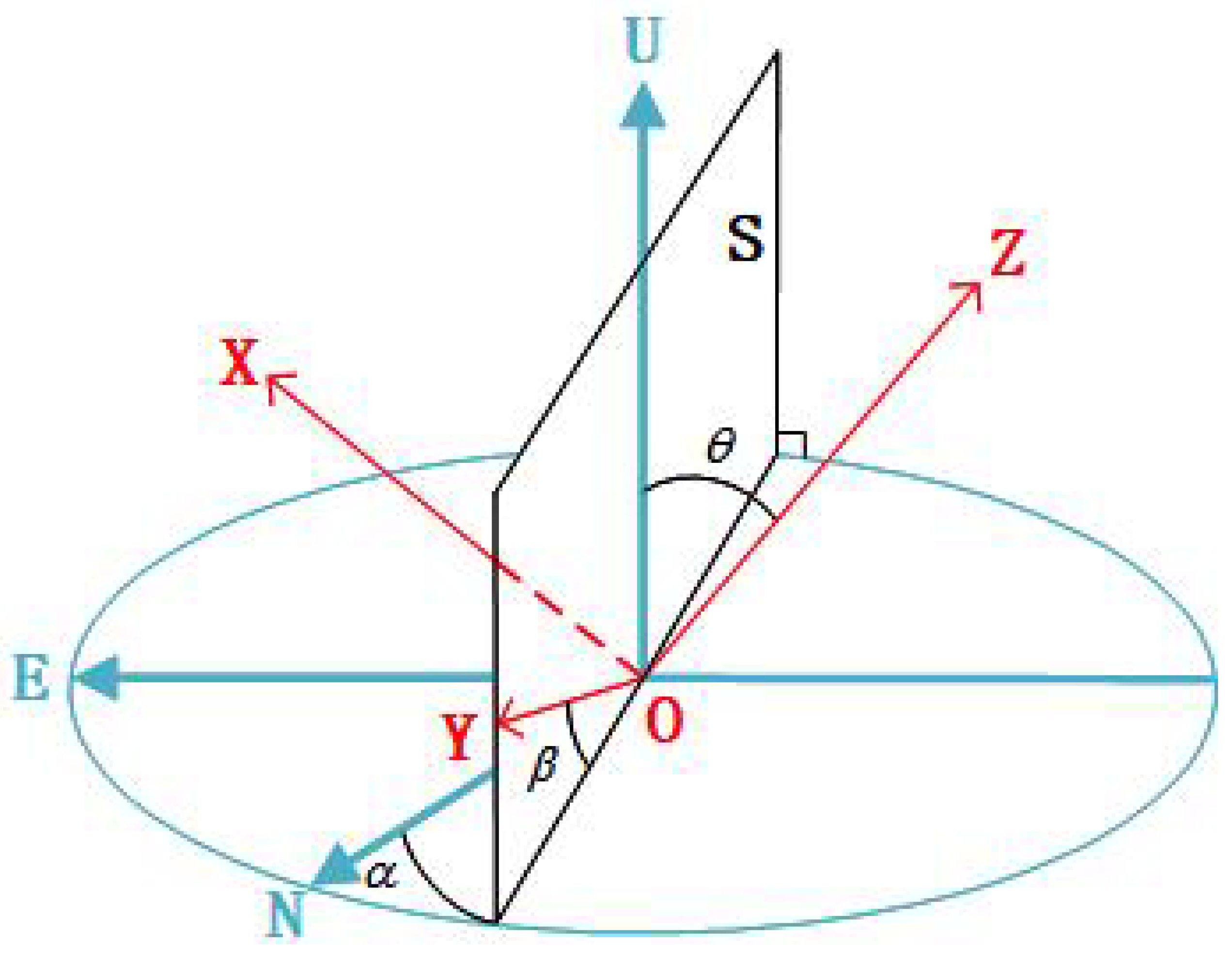
High-frequency motion error is mainly caused by the rotation of UAV platforms. This kind of rotation can be described by a static Euler angle [33]. The static Euler angle includes the yaw angle $\alpha$, pitch angle $\beta$, and roll angle $\theta$; these are defined relative to the stationary local coordinate system. A diagram of this is shown in Figure 1. The east-north-up (ENU) coordinate system is used as the local coordinate system. The $XYZ$ coordinate system is the carrier coordinate system. O is the origin of the two coordinate systems as well as the center of mass of the carrier. The right, front, and up directions of the UAV carrier, respectively, represent the positive direction of the X, Y, and Z axes of the carrier coordinate system. Yaw angle $\alpha$ is defined as the angle between the horizontal projection of the Y-axis and the N direction. Its positive direction is from north to west, and the range is $\left(-180{}^{\circ },180{}^{\circ }\right)$. Pitch angle $\beta$ is defined as the angle between the Y-axis and its horizontal projection, with the upward tilt direction of the carrier as the positive direction and the range being $\left(-90{}^{\circ },90{}^{\circ }\right)$. Roll angle $\theta$ is defined as the angle between the Z-axis and the vertical plane where the Y-axis lies, with the carrier tilting to the right as the positive direction and the range being $\left(-180{}^{\circ },180{}^{\circ }\right)$. Plane S is the vertical plane passing through the Y axis; it is perpendicular to the $EON$ plane.

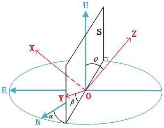
Figure 1. Schematic diagram of static Euler angles.

After defining the relative relationship between the carrier coordinate system and local coordinate system with the aircraft attitude information, the position of the antenna phase center (APC) in the local coordinate system can be calculated according to its position in the carrier coordinate system:

$$\begin{array}{c}\mathbf{X}=\left[\begin{array}{c}cos\alpha cos\theta +sin\theta sin\alpha sin\beta \\ sin\alpha cos\theta -sin\beta sin\theta cos\alpha \\ sin\theta cos\beta \end{array}\right]\\ \mathbf{Y}=\left[\begin{array}{c}cos\beta sin\alpha \\ cos\alpha cos\beta \\ sin\beta \end{array}\right]\\ \mathbf{Z}=\left[\begin{array}{c}-cos\theta sin\alpha sin\beta +sin\theta cos\alpha \\ -cos\theta cos\alpha sin\beta -sin\theta sin\alpha \\ cos\theta cos\beta \end{array}\right]\\ \tilde{\mathrm{A}}={\left[A_x{A}_y{A}_Z\right]}^T=p_x\mathbf{X}+p_y\mathbf{Y}+p_z\mathbf{Z},\end{array}$$

(1)

where the initial position of the antenna phase center in the platform coordinate system is ${\left[p_x{p}_y{p}_z\right]}^T$. According to (1), the high-frequency motion error caused by the jitter of the aircraft at each azimuth time u can be expressed as:

$$\mathbf{E}\left(u\right)=\tilde{\mathbf{A}}sin\left(2\pi {\tilde{f}}_{e}u+{\tilde{\phi }}_0\right),$$

(2)

where ${\tilde{f}}_e$ and ${\tilde{\phi }}_0$ represent the error frequency and the initial phase of the sinusoidal jitter of the aircraft, respectively.

In a mini-UAV-based SAR system, INS can be used to obtain the attitude information of the carrier platform at each moment. However, the INS with a high precision is too expensive to be widely used in UAV-based BiSAR systems, and the commonly used low-precision INS inevitably results in measurement error of the aircraft attitude. When the carrier frequency is high, such as in Ku band, a millimeter-level measurement error will cause a large phase error (5 mm error can cause 1.67 rad phase error in a 16 GHz system). Therefore, it is infeasible to simply use the information from INS to compensate for high-frequency motion errors.

2.1.2. High-Frequency Motion Error in BiSAR

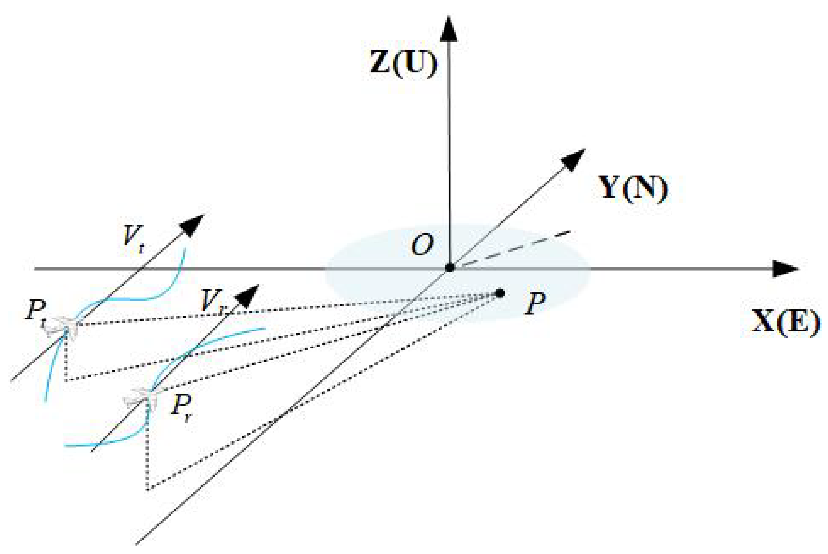
A configuration of BiSAR systems based on UAV platforms is shown in Figure 2. $P_t$, $P_r$, $V_t$, and $V_r$ are the position and velocity of the transmitter and receiver. O is the origin point of the coordinate system as well as the center of the scene. $\mathbf{P}$ is the target position. The coordinates are defined in the ENU coordinate system, which is the same in Figure 1. The blue curve is the actual trajectory of the APC and is greatly affected by the environment.

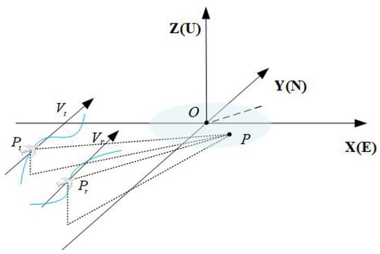
Figure 2. The configuration of the UAV-based BiSAR systems.

The slant range error of target $\mathbf{P}$ can be modeled as the sum of two parts, low-frequency error component and high-frequency error component:

$$\Delta R\left(u,\mathbf{P}\right)=\Delta R_{low}\left(u,\mathbf{P}\right)+\Delta R_{high}\left(u,\mathbf{P}\right),$$

(3)

where u is the slow time, $\Delta R_{low}$ is the low-frequency error component, and $\Delta R_{high}$ is the high-frequency error component. The MOCO for low-frequency motion error in mini-UAV-based BiSAR has been solved [12]. Regarding high-frequency motion error, based on (2), $\Delta R_{high}\left(u,\mathbf{P}\right)$ can be expressed as:

$$\begin{array}{c}\Delta R_{high}\left(u,\mathbf{P}\right){=\tilde{\mathrm{A}}}_{\mathbf{T}}^{\mathbf{T}}{\mathsf{\Phi }}_{\mathbf{TP}}^{}·sin(2\pi {\tilde{f}}_{eT}u+{\tilde{\phi }}_{0T})+{\tilde{\mathrm{A}}}_{\mathbf{R}}^{\mathbf{T}}{\mathsf{\Phi }}_{\mathbf{RP}}^{}·sin(2\pi {\tilde{f}}_{eR}u+{\tilde{\phi }}_{0R})\hfill \\ ={\tilde{a}}_T·sin(2\pi {\tilde{f}}_{eT}u+{\tilde{\phi }}_{0T})+{\tilde{a}}_R·sin(2\pi {\tilde{f}}_{eR}u+{\tilde{\phi }}_{0R}),\hfill \end{array}$$

(4)

where ${\mathsf{\Phi }}_{\mathbf{TP}}^{}$ represents the unit vector of the line-of-sight (LOS) direction of the transmitter to target $\mathbf{P}$ and ${\mathsf{\Phi }}_{\mathbf{RP}}^{}$ represents the unit vector of the LOS direction of the receiver to target $\mathbf{P}$. The subscripts ${}_T$ and ${}_R$ represent the transmitter and receiver, respectively. The expressions of ${\mathsf{\Phi }}_{\mathbf{TP}}^{}$ and ${\mathsf{\Phi }}_{\mathbf{RP}}^{}$ are:

$${\mathsf{\Phi }}_{\mathbf{TP}}^{}=\frac{\mathbf{P}-\mathbf{T}}{\left|\mathbf{P}-\mathbf{T}\right|},{\mathsf{\Phi }}_{\mathbf{RP}}^{}=\frac{\mathbf{P}-\mathbf{R}}{\left|\mathbf{P}-\mathbf{R}\right|}.$$

(5)

For synthetic aperture time T, the frequency resolution along the azimuth direction is ${}^1/{}_T$. When T is relatively short, it is hard to distinguish ${\tilde{f}}_{eT}$ and ${\tilde{f}}_{eR}$ along the azimuth direction. In mini-UAV-based SAR systems, the frequency of the motion error is always a few Hz, i.e., their frequencies are not drastically different. Thus, two high-frequency error components are likely to have similar frequencies and be coupled with each other, which will greatly increase the difficulty of motion compensation. Therefore, it is necessary to deal with this special situation. Thus, when the error frequencies are similar, i.e., ${\tilde{f}}_{eT}\approx {\tilde{f}}_{eR}=f_e$, (4) can be simplified as:

$$\begin{array}{cc}\Delta R_{high}\left(u,\mathbf{P}\right)\hfill & ={\tilde{a}}_T·sin(2\pi {\tilde{f}}_{eT}u+{\tilde{\phi }}_{0T})+{\tilde{a}}_R·sin(2\pi {\tilde{f}}_{eR}u+{\tilde{\phi }}_{0R})\hfill \\ \hfill & ={\tilde{a}}_T\left(cos\left(2\pi {\tilde{f}}_{eT}u\right)cos{\tilde{\phi }}_{0T}-sin\left(2\pi {\tilde{f}}_{eT}u\right)sin{\tilde{\phi }}_{0T}\right)\hfill \\ \hfill & +{\tilde{a}}_R\left(cos\left(2\pi {\tilde{f}}_{eR}u\right)cos{\tilde{\phi }}_{0R}-sin\left(2\pi {\tilde{f}}_{eR}u\right)sin{\tilde{\phi }}_{0R}\right)\hfill \\ \hfill & =\left({\tilde{a}}_{T}cos{\tilde{\phi }}_{0T}+{\tilde{a}}_{R}cos{\tilde{\phi }}_{0R}\right)cos\left(2\pi {\tilde{f}}_{eT}u\right)-\left({\tilde{a}}_{T}sin{\tilde{\phi }}_{0T}+{\tilde{a}}_{R}sin{\tilde{\phi }}_{0R}\right)sin\left(2\pi {\tilde{f}}_{eR}u\right)\hfill \\ \hfill & =F_{1}cos\left(2\pi f_{e}u\right)-F_{2}sin\left(2\pi f_{e}u\right)\hfill \\ \hfill & =\sqrt{{F_1}^2+{F_2}^2}cos\left(2\pi f_{e}u+{\phi }_0\right)\hfill \\ \hfill & =acos\left(2\pi f_{e}u+{\phi }_0\right)\hfill \end{array}$$

(6)

where

$$\begin{array}{c}{F}_1=a_{T}cos{\tilde{\phi }}_{0T}+a_{R}cos{\tilde{\phi }}_{0R},\hfill \\ F_2=a_{T}sin{\tilde{\phi }}_{0T}+a_{R}sin{\tilde{\phi }}_{0R},\hfill \\ a=\sqrt{{F_1}^2+{F_2}^2}\hfill \\ {\phi }_0=arccos\left(\frac{F_1}{\sqrt{{F_1}^2+{F_2}^2}}\right).\hfill \end{array}$$

(7)

Based on (6) and (7), the high-frequency motion errors are coupled with each other and cannot be separated. Thus, the motion error of the platform cannot be estimated and the traditional MOCO algorithm based on parameter estimation cannot be used here.

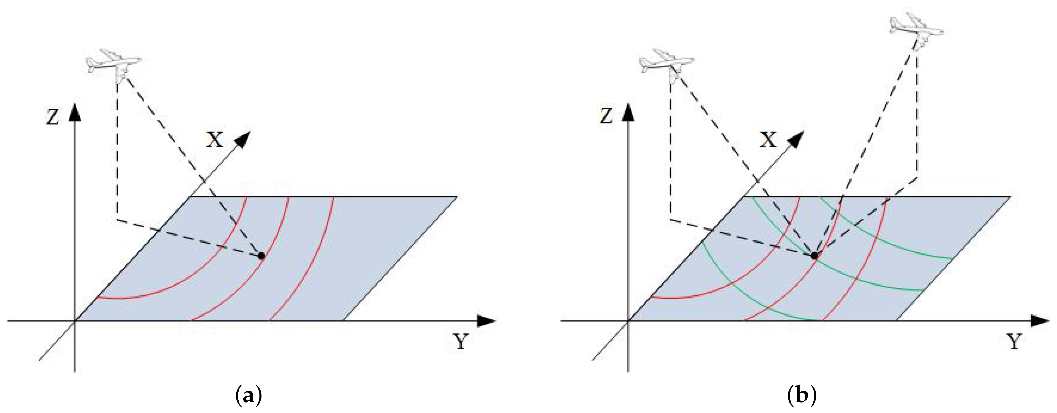
Based on (6), the parameters of high-frequency errors consist of amplitude a, frequency $f_e$, and initial phase ${\phi }_0$. The frequency value $f_e$ is a constant value across the whole scene, but the spatial variance of the amplitude a and the initial phase ${\phi }_0$ must be considered. For a monostatic system, spatial variance is introduced only by one radar platform and it is simply along a single direction. As shown in Figure 3a, the red contour map shows the spatial variance of a monostatic system. For a bistatic configuration, as is shown in Figure 3b, the red and the green spatial variance contour maps correspond to the transmitter and receiver, respectively. The spatial variance of the system error is the superposition of the spatial variance of the transmitter and receiver, i.e., the superposition of the red lines and green lines. Thus, a new bistatic spatial variance compensation algorithm needs to be proposed for this condition.

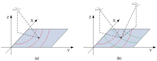
Figure 3. Spatial variance of high frequency motion error of monostatic and bistatic SAR system. (a) is the monostatic system. (b) is the bistatic system.

2.1.3. System Signal Model

Based on the former derivations, the slant range with motion errors can be expressed as:

$$R\left(u,\mathbf{P}\right)=R_0\left(u,\mathbf{P}\right)+\Delta R\left(u,\mathbf{P}\right),$$

(8)

where $R_0\left(u,\mathbf{P}\right)$ is the slant range calculated using the platform motion information recorded by INS. For common radar systems, the transmitted signal is:

$$s\left(t,u\right)=rect\left[\frac{t-R\left(u\right)/c}{T_p}\right]exp\left(j\pi K_r{\left(t-\frac{R\left(u\right)}{c}\right)}^2\right)rect\left(\frac{u}{T_{\mathrm{int}}}\right)exp\left(-j\frac{2\pi R\left(u\right)}{\lambda }\right).$$

(9)

The amplitude of the high-frequency motion error is generally in the order of millimeters; thus, the influence on the RCM can be ignored. After RCM error is introduced by the low-frequency motion error compensation [34,35] and range pulse compression, the signal can be expressed as:

$$s_1\left(u,t,\mathbf{P}\right)=G\left(u\right)sinc\left\{B\left[t-2R_0/c\right]\right\}·exp\left\{-j\frac{2\pi }{\lambda }\left[\left(R_0\left(u,\mathbf{P}\right)+\Delta R\left(u,\mathbf{P}\right)\right)\right]\right\}.$$

(10)

Substituting (3) into (10), the signal expression before azimuth processing is:

$$\begin{array}{c}{s}_1\left(u,\mathbf{P}\right)=G\left(u\right)·sinc\left\{B\left[t-2R_0/c\right]\right\}·\hfill \\ exp\left\{-j\frac{2\pi }{\lambda }\left(R\left(u,\mathbf{P}\right)+\Delta R_{low}\left(u,\mathbf{P}\right)+asin(2\pi f_{e}u+{\phi }_0)\right)\right\}.\hfill \end{array}$$

(11)

Thus, the azimuth phase with motion error is obtained. The spatial variant motion error will be compensated for in the next section.

2.2. High-Frequency MOCO for BISAR

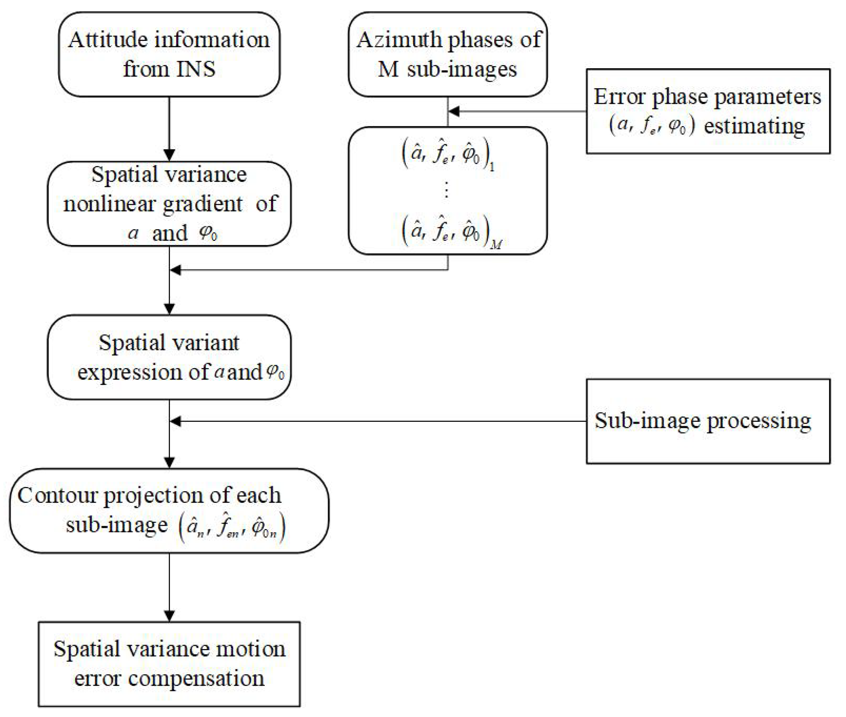
According to the analysis shown in Section 2, the parameters of the platforms’ motion error, i.e., $\tilde{\mathbf{A}},{\tilde{f}}_e,{\tilde{\phi }}_0$, cannot be estimated. In this subsection, the parameters of the azimuth phase of some subimages are estimated; then, a nonlinear gradient is introduced to describe the bistatic spatial variance. Finally, the high-frequency motion error of the whole scene is compensated through contour projection. The flowchart is shown in Figure 4.

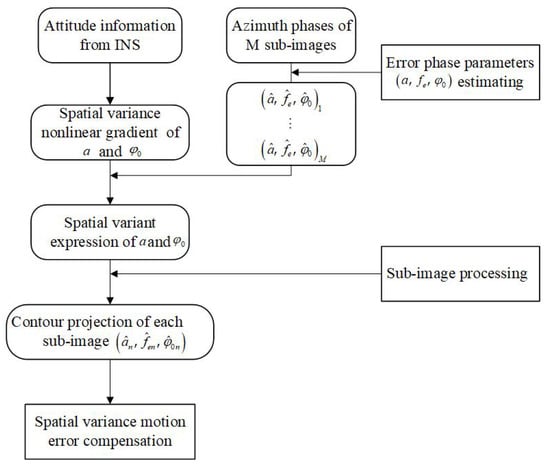
Figure 4. The flowchart of the proposed spatial variant high-monofrequency MOCO algorithm.

2.2.1. High-Frequency Phase Error Parameters Estimation

In order to compensate for the spatial variant high-monofrequency motion error, first, the phase error parameters need to be estimated. There has been some research about the parameter estimation of high-frequency phase error [25,26,27,28]. Based on M sets of strong points or subimages, M sets of phase error parameters can be obtained, where each set of parameters includes an amplitude, an error frequency, and an initial phase, as shown in (12).

$${\left({\widehat{a}}_1,{\widehat{f}}_{e1},{\widehat{\phi }}_{01}\right)}_1\cdots {\left({\widehat{a}}_M,{\widehat{f}}_{eM},{\widehat{\phi }}_{0M}\right)}_M$$

(12)

For the error frequency, based on the (6) and (7), it has no spatial variance. Thus, the final error frequency can be obtained using the weighted average.

$${\widehat{f}}_e=\frac{{\displaystyle \sum _{m=1}^M}\left(f_{max}\left(S_m\right){\widehat{f}}_{em}\right)}{{\displaystyle \sum _{m=1}^M}\left(f_{max}\left(S_m\right)\right)},$$

(13)

where $f_{max}\left(S_m\right)$ is the maximum amplitude of the mth subimage.

However, for the amplitude and initial phase, the estimated parameters are the result of coupling two sets of high-frequency errors, and the actual motion error parameters of the platforms cannot be calculated to compensate for the spatial variant phase error. The following section proposes a new error compensation algorithm.

2.2.2. Spatial Variant Model Establishment

Based on (6) and (7), the spatial variance of the amplitude a and the initial phase ${\phi }_0$ of the high-frequency motion error need to be considered. Because the motion errors are coupled with each other, they cannot be compensated for through the traditional trajectory estimation algorithm. A new bistatic spatial variance compensation algorithm is proposed in this subsection.

1.

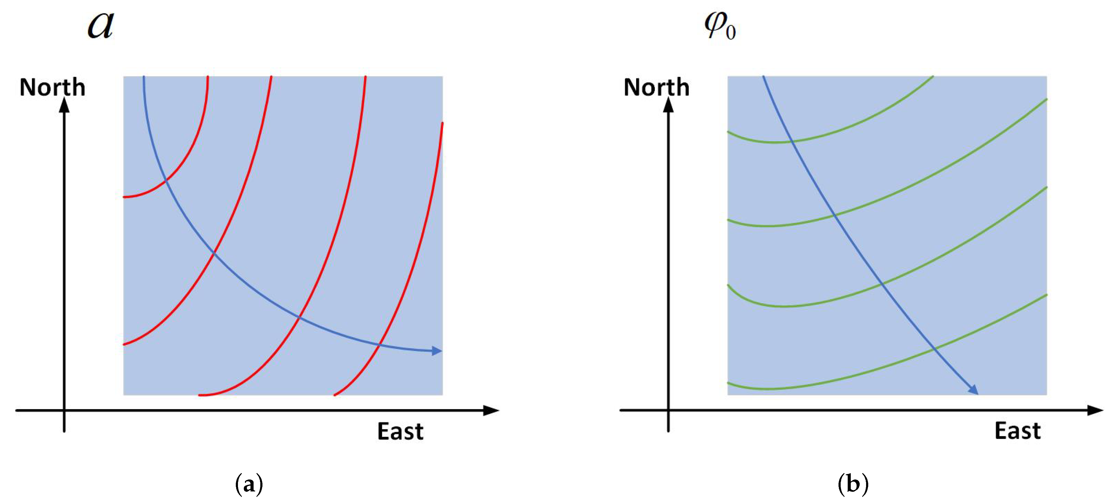
First, the approximate UAV’s attitude information can be obtained through the INS, which is written as:

$$\overline{\mathbf{A}}={\left[{\overline{A}}_x{\overline{A}}_y{\overline{A}}_Z\right]}^T.$$

(14)

Limited by the accuracy of the INS, the estimated value $\overline{\mathbf{A}}$ cannot be directly used for motion error compensation, but it can be used to obtain the approximate direction of the spatial variance of the high-frequency motion error parameters. Based on the system configuration, ${\mathsf{\Phi }}_{\mathbf{TP}}^{}$ and ${\mathsf{\Phi }}_{\mathbf{RP}}^{}$ can be calculated. Then, combining them with (7), the approximate a and ${\phi }_0$ of each position can be calculated. The diagram is shown in Figure 5. The red line in Figure 5a is the contour of a and the green line in Figure 5b is the contour of ${\phi }_0$. The contour line will change with the system configuration and error parameters.

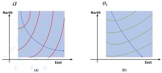Figure 5. The contour and the nonlinear gradient of the amplitude a and initial phase ${\phi }_0$. (a) is the result of a. (b) is the result of ${\phi }_0$.

2.

Second, calculate the nonlinear gradient of the a and ${\phi }_0$ for the whole scene. For the position $\left(x,y\right)$, the amplitude is $f_a\left(x,y\right)$ and the initial phase is $f_{\phi }\left(x,y\right)$. The gradient direction can be calculated as:

$$\begin{array}{c}{\gamma }_a\left(x,y\right)=arctan\left[\frac{g_{ya}}{g_{xa}}\right]\hfill \\ {\gamma }_{\phi }\left(x,y\right)=arctan\left[\frac{g_{y\phi }}{g_{x\phi }}\right],\end{array}$$

(15)

where $\gamma$ is the gradient direction, and:

$$\begin{array}{c}{g}_{xa}=\partial f_a/\partial x,g_{ya}=\partial f_a/\partial y\hfill \\ g_{x\phi }=\partial f_{\phi }/\partial x,g_{y\phi }=\partial f_{\phi }/\partial y.\end{array}$$

(16)

The blue line in Figure 5 indicates the nonlinear gradient of the spatial variance. The error parameters vary the most violently along the direction of the spatial variance gradient. Therefore, the model based on the gradient information can greatly describe the spatial variance of the scene, which is more accurate than modeling along range or azimuth direction. Since the bistatic spatial variance is more complex than that of monostatic condition, the proposed variance model is necessary under the BiSAR condition.

3.

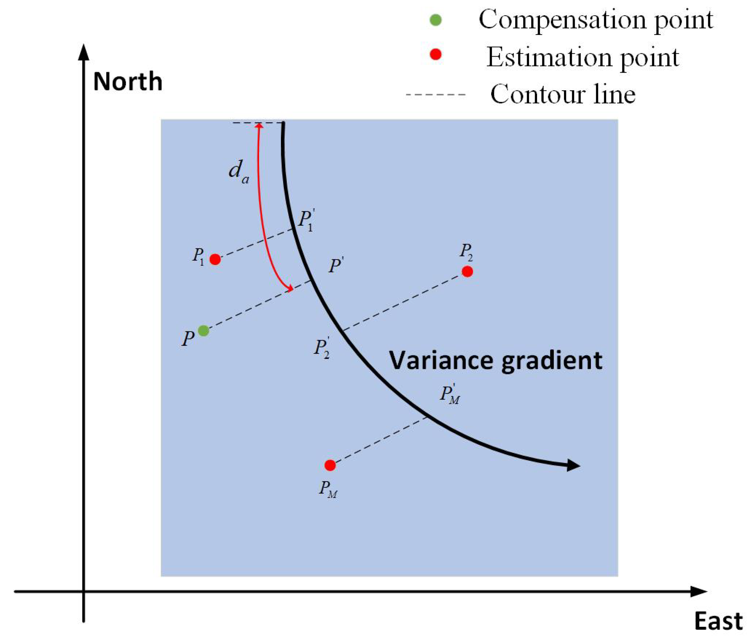
Third, estimate the parameters of the high-frequency phase error in several subimages. It is believed that the error parameters on one contour are the same; thus, target $\mathbf{P}$ can be projected to the gradient along the contour line. A diagram of this is shown in Figure 6. ${\mathbf{P}}_1,{\mathbf{P}}_2,{\mathbf{P}}_M$ are the estimation positions and ${{\mathbf{P}}_1}^{\prime },{{\mathbf{P}}_2}^{{}^{\prime }},{{\mathbf{P}}_M}^{\prime }$ are the projection points of ${\mathbf{P}}_1,{\mathbf{P}}_2,{\mathbf{P}}_M$, respectively. In this way, based on M sets of estimation results, M sets of error parameters for the nonlinear spatial variance gradient can be obtained.

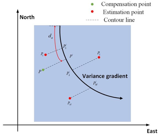Figure 6. Nonlinear spatial variance gradient projection model in a UAV-based BiSAR system.

4.

Fourth, based on M sets of estimation results, a and ${\phi }_0$ can be obtained at each point on the gradient. Here, the second-order fit is selected, which can be expressed as:

$$\begin{array}{c}a\left({\mathbf{P}}^{{}^{\prime }}\right)=m_0+m_1{d}_a\left({\mathbf{P}}^{{}^{\prime }}\right)+m_2{d}_a^2\left({\mathbf{P}}^{{}^{\prime }}\right)\hfill \\ {\phi }_0\left({\mathbf{P}}^{{}^{\prime }}\right)=n_0+n_1{d}_{\phi }\left({\mathbf{P}}^{{}^{\prime }}\right)+n_2{d}_{\phi }^2\left({\mathbf{P}}^{{}^{\prime }}\right),\hfill \end{array}$$

(17)

where $d_a$ is the distance from ${\mathbf{P}}^{{}^{\prime }}$ to the origin point O of the amplitude gradient $d_{\phi }$ is the distance from ${\mathbf{P}}^{{}^{\prime }}$ to the origin point O of the initial phase gradient. $d_a$ is shown as the red line in Figure 6 as an example. The coefficients can be calculated as:

$$\begin{array}{c}{m}_0,m_1,m_2=\underset{m_0,m_1,m_2}{argmin}\frac{1}{M}{\displaystyle \sum _{i=1}^M}\left(a\left({\mathbf{P}}_i^{{}^{\prime }}\right)-{\widehat{a}}_i\right)\hfill \\ n_0,n_1,n_2=\underset{n_0,n_1,n_2}{argmin}\frac{1}{M}{\displaystyle \sum _{i=1}^M}\left({\phi }_0\left({\mathbf{P}}_i^{{}^{\prime }}\right)-{\widehat{\phi }}_{0i}\right),\hfill \end{array}$$

(18)

Now, a and ${\phi }_0$ at each point on the nonlinear gradient are obtained.

5.

Fifth, divide the whole image into subimages with the premise that the greatest difference in phase error is less than $\pi /4$. Then, project the center of each subimage onto the nonlinear spatial variant gradient. The high-frequency error parameter of each subimage is same as the projection point on the spatial variant gradient. In Figure 6, $\mathbf{P}$ is the center of one of the subimages that needs to be compensated for, and the error parameters can be obtained through ${\mathbf{P}}^{\prime }$.

2.2.3. High-Frequency Motion Error Compensation

In order to eliminate the effect of high-frequency errors on azimuth focusing, a compensation signal needs to be constructed. Let the estimation result of the $n^{th}$ subscene be $\left({\widehat{a}}_n,{\widehat{f}}_e,{\widehat{\phi }}_{0n}\right)$. The compensation signal can be expressed as:

$$f_{comp}=exp\left\{j\frac{2\pi }{\lambda }\left({\widehat{a}}_{n}sin(2\pi {\widehat{f}}_{e}u+{\widehat{\phi }}_{0n})\right)\right\}.$$

(19)

Then, multiplying (11) and (19), the high-frequency motion error can be compensated for; the signal can be expressed as:

$$s_1\left(u,\mathbf{P}\right)=G\left(u\right)exp\left\{-j\frac{2\pi }{\lambda }\left(R\left(u,\mathbf{P}\right)+\Delta R_{low}\left(u,\mathbf{P}\right)+\Delta \varphi \right)\right\},$$

(20)

where $\Delta \varphi$ is the residual high-frequency phase error, which will not affect the image result. After the high-frequency error phase compensation, the traditional MOCO algorithm can be used to compensate for the residual low-frequency error phase. By now, the low-frequency and high-frequency motion errors of the UAV-based bistatic system have both been compensated for.

3. Experiment and Results

In this section, simulation and raw data are used to verify the proposed algorithm.

3.1. Simulation and Analysis

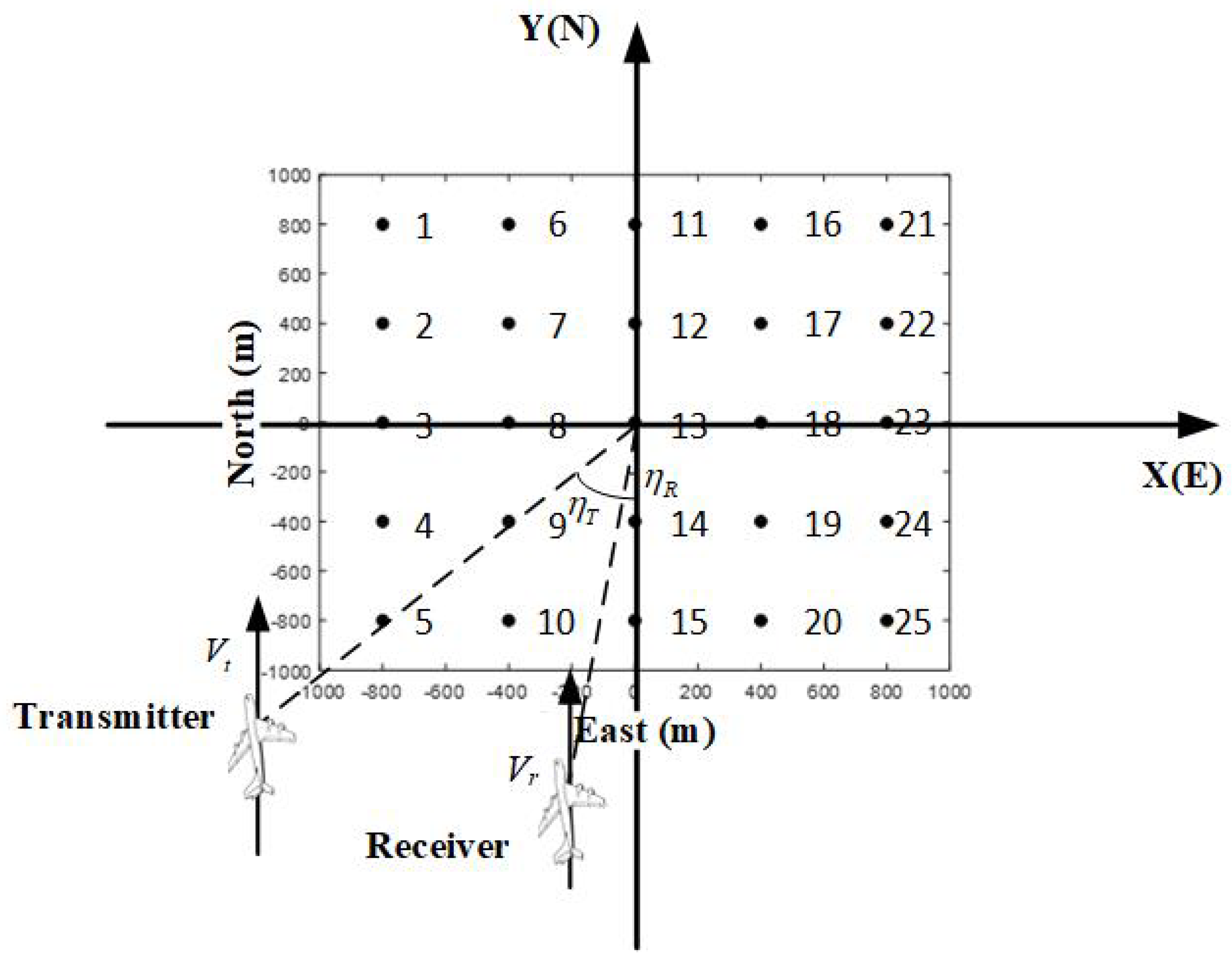
In order to verify the effectiveness of the algorithm, first, simulation experiment is processed. The simulation parameters are shown in Table 1. The coordinate values correspond to the $XYZ$(ENU) axis, which is defined in Figure 2. The imaging targets are set as a $5\times 5$ point array evenly distributed in an area of 1600 m × 1600 m range. The number of each target point and the bistatic configuration are shown in Figure 7. ${\eta }_{\mathrm{T}},{\eta }_R$ are the squinted angle of transmitter and receiver, respectively. The center target is at the $\left[0,0,0\right]$, which is also the origin of the coordinate system. In the simulation, the transmitter and receiver illuminate the center of the scene and the echoes from all targets can be received.

Table 1. Simulation parameters.

Parameters	Values
Transmitter position	$\left[-1300;-1300;500\right]$ m
Transmitter velocity	$\left[0;20;0\right]$ m/s
Transmitter acceleration	$\left[0.2;0.2;0.2\right]$ m/s${}^2$
Transmitter squinted angle	${45}^{\circ }$
Receiver position	$\left[-87;-1000;500\right]$ m
Transmitter velocity	$\left[0;15;0\right]$ m/s
Transmitter acceleration	$\left[0.2;0.2;0.2\right]$ m/s${}^2$
Transmitter squinted angle	${85}^{\circ }$
Radar wavelength	0.019 m
Bandwidth	120 MHz
Synthetic aperture time	1.5 s
PRF	1250 Hz
The center of the antenna beam pointing	$\left[0;0;0\right]$ m

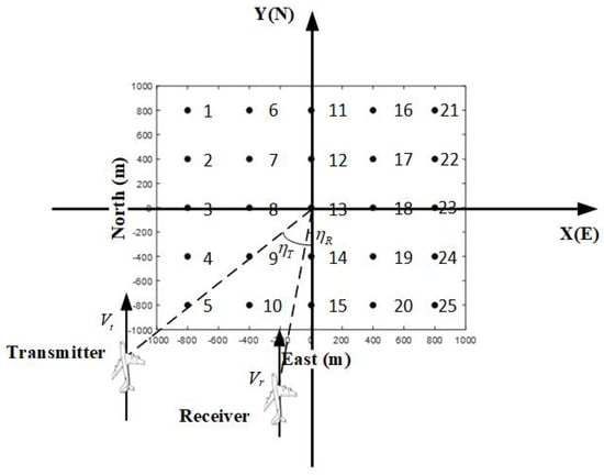
Figure 7. The targets of the simulation experiment and the bistatic configuration.

In the simulation experiment, the high-frequency error parameters are directly given; they are shown in Table 2.

Table 2. High-frequency error parameters in simulation.

	High-Frequency Error
	Amplitude H (mm)	Frequency ${\mathit{f}}_{\mathit{e}}$ (Hz)	Initial Phase ${\tilde{\mathit{\phi }}}_0\left({}^{\circ }\right)$
Transmitter	$\left[1.1;4.5;3.4\right]$	5	20
Receiver	$\left[7.5;4.3;3.2\right]$	5	140

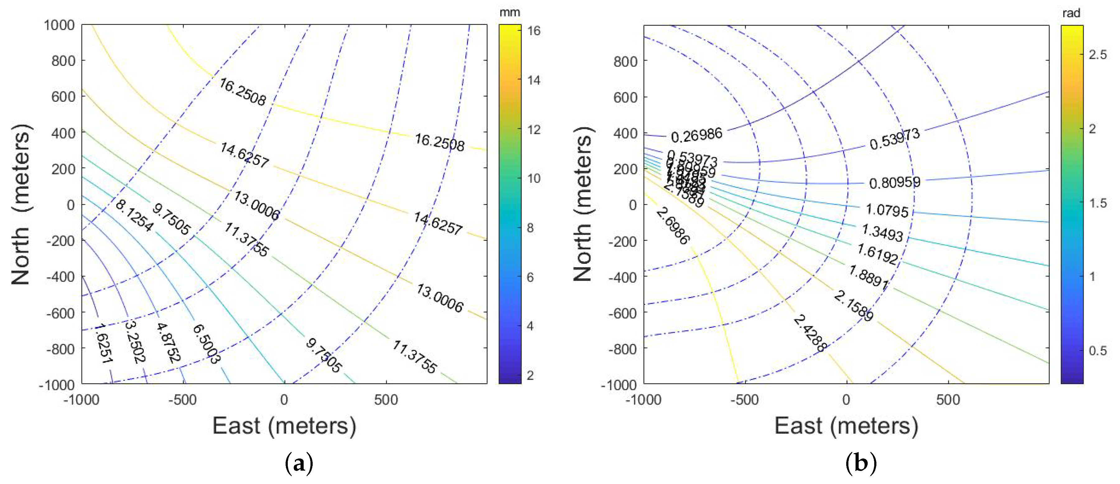
The spatial variance of the amplitude and initial phase in the whole imaging scene is simulated as shown in Figure 8, where Figure 8a shows the simulation of the spatial variance of the amplitude whose unit is mm. Figure 8b shows the spatial variance of the initial phase whose unit is rad. The spatial variance is shown as the contour lines, and the values are attached. The minimum of them is 0 to represent the change better. The blue dotted lines are the gradient lines. In this experiment, the gradient line that passes through the scene center is used as the projection line.

Figure 8. The bistatic spatial variance of the amplitude and initial phase under simulation. (a) is the result of amplitude. (b) is the result of the initial phase. The contour lines are shown as solid lines with values attached and the gradient lines are shown as blue dotted lines.

Then, the high-frequency motion error parameters of several strong scattering points are estimated. Targets 3, 8, 14, and 17 are used to estimate the phase error parameters. The parameter estimation results are shown in Table 3.

Table 3. Parameter estimation results of selected targets in the simulation experiment.

Target	Phase Amplitude $\widehat{\mathit{a}}$ (rad)	Frequency ${\widehat{\mathit{f}}}_{\mathit{e}}$ (Hz)	Initial Phase ${\widehat{\mathit{\phi }}}_0\left({}^{\circ }\right)$
3	0.24	4.99	5.22
8	0.90	4.99	15.93
14	1.12	4.99	51.89
17	2.53	4.99	98.48

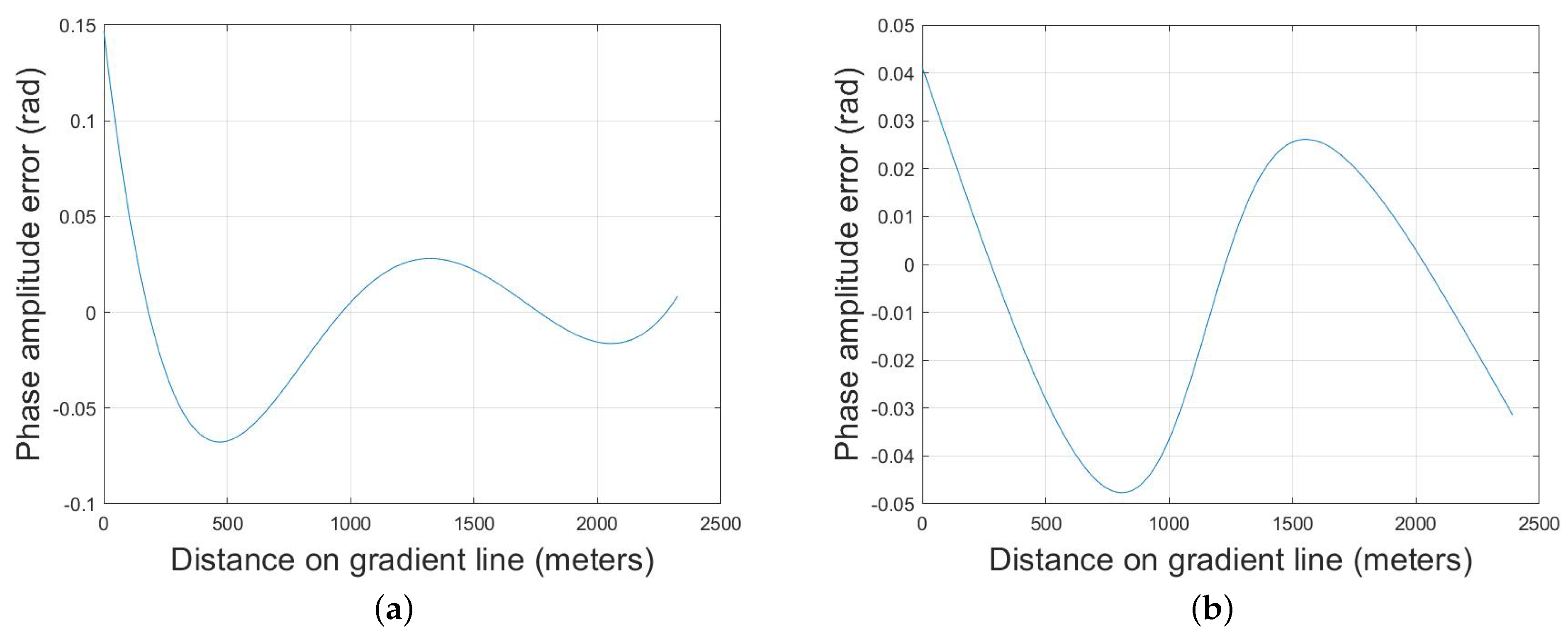
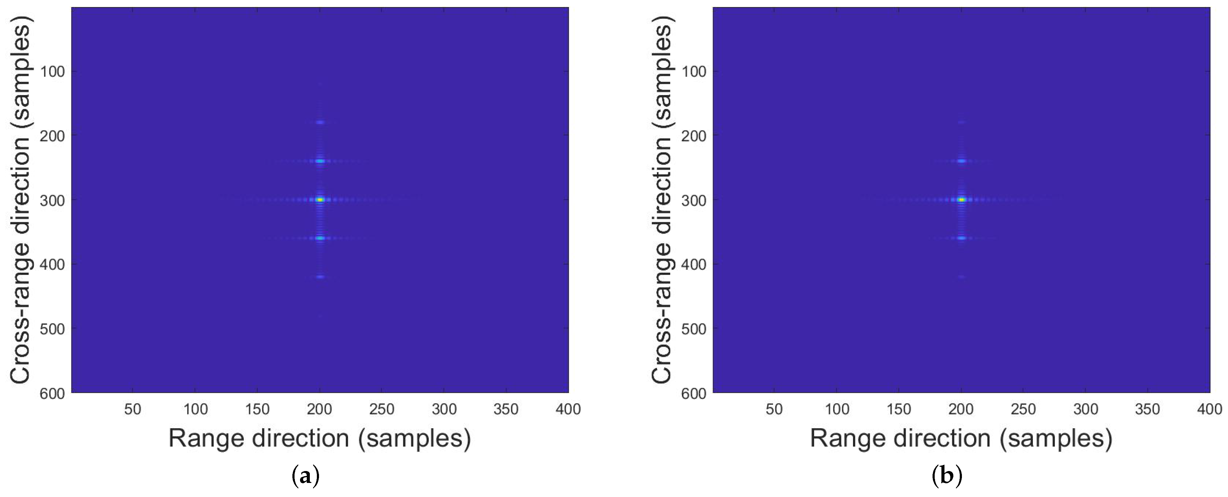
Next, the proposed method is used to fit the amplitude and initial phase along the nonlinear spatial variant gradient. Figure 9 shows the fitting curve error, where Figure 9a is the fitted result of error amplitude and Figure 9b is the fitted result of the error initial phase. The X axis is the distance along the gradient and the Y axis is the error on the azimuth phase. It can be seen that the accuracy of the fitting reuslt is high enough.

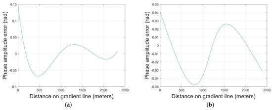
Figure 9. The difference between the fitted value and the true value of the parameter on the gradient. (a) is the result of amplitude. (b) is the result of the initial phase.

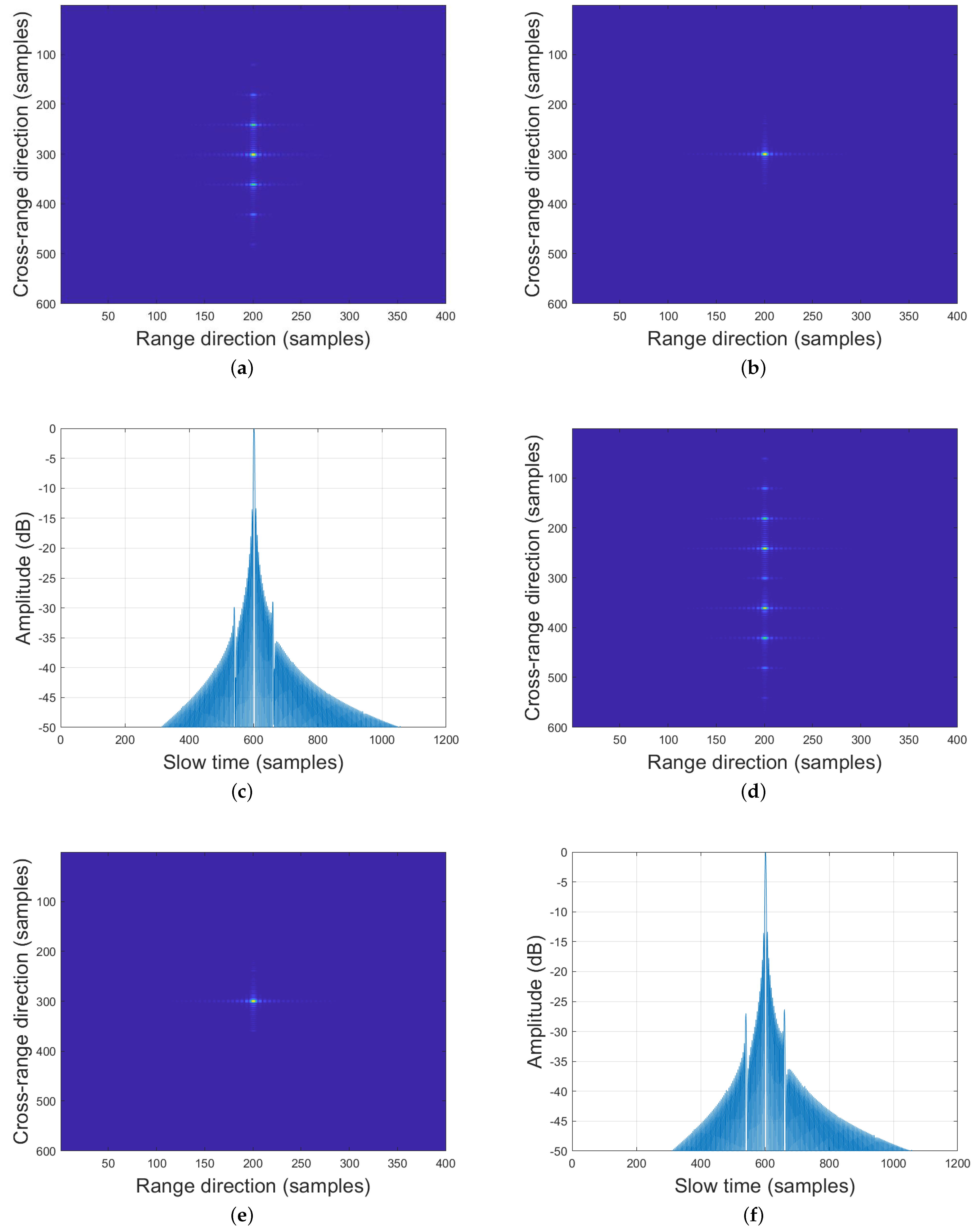
Taking target points 1 and 25 as examples, the results before and after motion error compensation are shown in Figure 10. Figure 10a–c show the simulation results of target 1, the image results before and after MOCO, and the cross-range result after MOCO. Figure 10d–f shows the simulation results of target 25. In the compensation results, false targets have been well reduced.

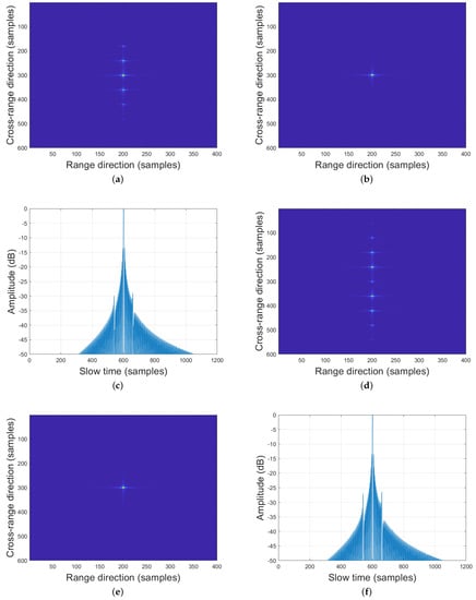
Figure 10. Compensation results. (a–c) show the simulation of target 1, the image result before and after MOCO, and the cross-range result after MOCO. (d–f) show the simulation results of target 25.

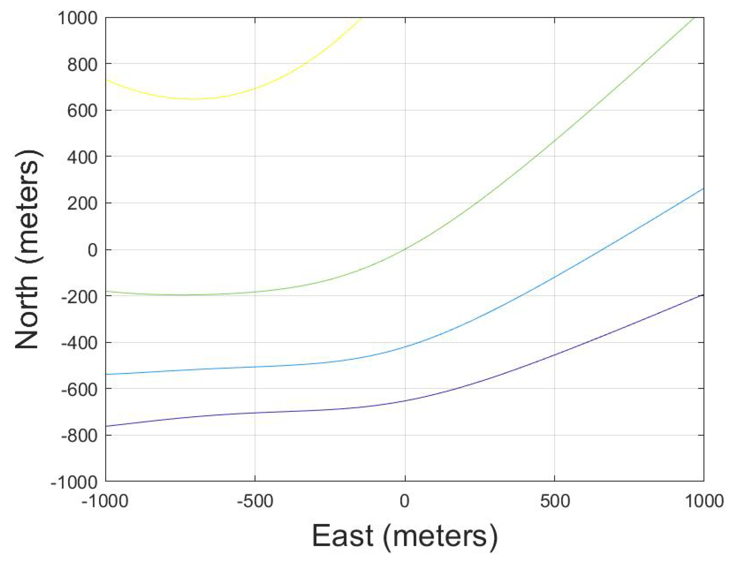
Then, the high-frequency compensation algorithm [11] and spatial variance compensation algorithm [23] are used to compensate this high-monofrequency motion error. The spatial variance model is established along the range direction. The range direction in the simulation configuration is shown in Figure 11. The line passing through the origin is used as the projection line. It can be seen that it is quite different from the proposed gradient line. Then, the final compensation results of target 1 and 25 and are shown in Figure 12. It can be seen there are still false targets appearing on the image results.

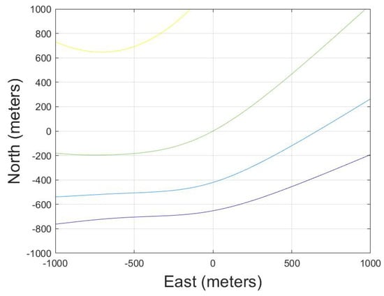
Figure 11. The range direction in the simulation configuration.

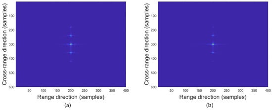
Figure 12. The compensation results of the traditional algorithm [11,23]. (a) is the result of target 1. (b) is the result of target 25.

In order to better prove the improvement brought by the proposed algorithm under this condition, the compensation effect of the false targets of different algorithms are shown in Table 4. Take the four points of the furthest distance as examples; the values in the table indicate the amplitude difference between the false target position and the main lobe. For the proposed algorithm, it can be seen that the false targets have been greatly suppressed after motion compensation, and the suppression effect is above 26 dB. Furthermore, all of the targets have been well compensated, which verifies that the spatial variance of the motion error have been solved well. However, for the traditional algorithm [11,23], the worst compensation effect is only around 8 dB. The results show that traditional compensation algorithm cannot be used in this condition.

Table 4. Compensation results of the target 1, 5, 21, and 25.

Target	Target 1	Target 5	Target 21	Target 25
Proposed algorithm	−28.03 dB	−27.33 dB	−27.63 dB	−26.58 dB
Traditional algorithm	−8.34 dB	−15.88 dB	−14.24 dB	−12.33 dB

3.2. Raw Data Processing

In this subsection, an experiment adopting the mini-UAV-based BiSAR is carried out. The system is Ku-band and the antenna adopts vertical polarization. The system parameters are shown in Table 5. The definition of the coordinates is the same as that in the simulation. The experimental area is an island that contains two transponders, a hut block, a wharf, and a road. The center point $\left[0,0,0\right]$ is defined at the wharf. During the image processing, the synthetic aperture is small compared to the radar operating distance such that it can be considered that the fields of view remain unchanged.

Table 5. Experiment parameters.

Parameters	Values
Transmitter position	$\left[-937.7;-2961;523\right]$ m
Transmitter velocity	$\left[22.16;0.08;-0.10\right]$ m/s
Transmitter acceleration	$\left[0.13;0.08;0.06\right]$ m/s${}^2$
Transmitter squinted angle	${17}^{\circ }$
Receiver position	$\left[-700.5;-2173;412\right]$ m
Transmitter velocity	$\left[21.22;0.28;-0.03\right]$ m/s
Transmitter acceleration	$\left[0.19;-0.13;-0.11\right]$ m/s${}^2$
Transmitter squinted angle	${25}^{\circ }$
Radar wavelength	0.019 m
Bandwidth	120 MHz
Synthetic aperture time	1.5 s
PRF	1250 Hz
The center of the antenna beam pointing	$\left[0;0;0\right]$ m
APC position	$\left[0;21.4;62\right]$ mm

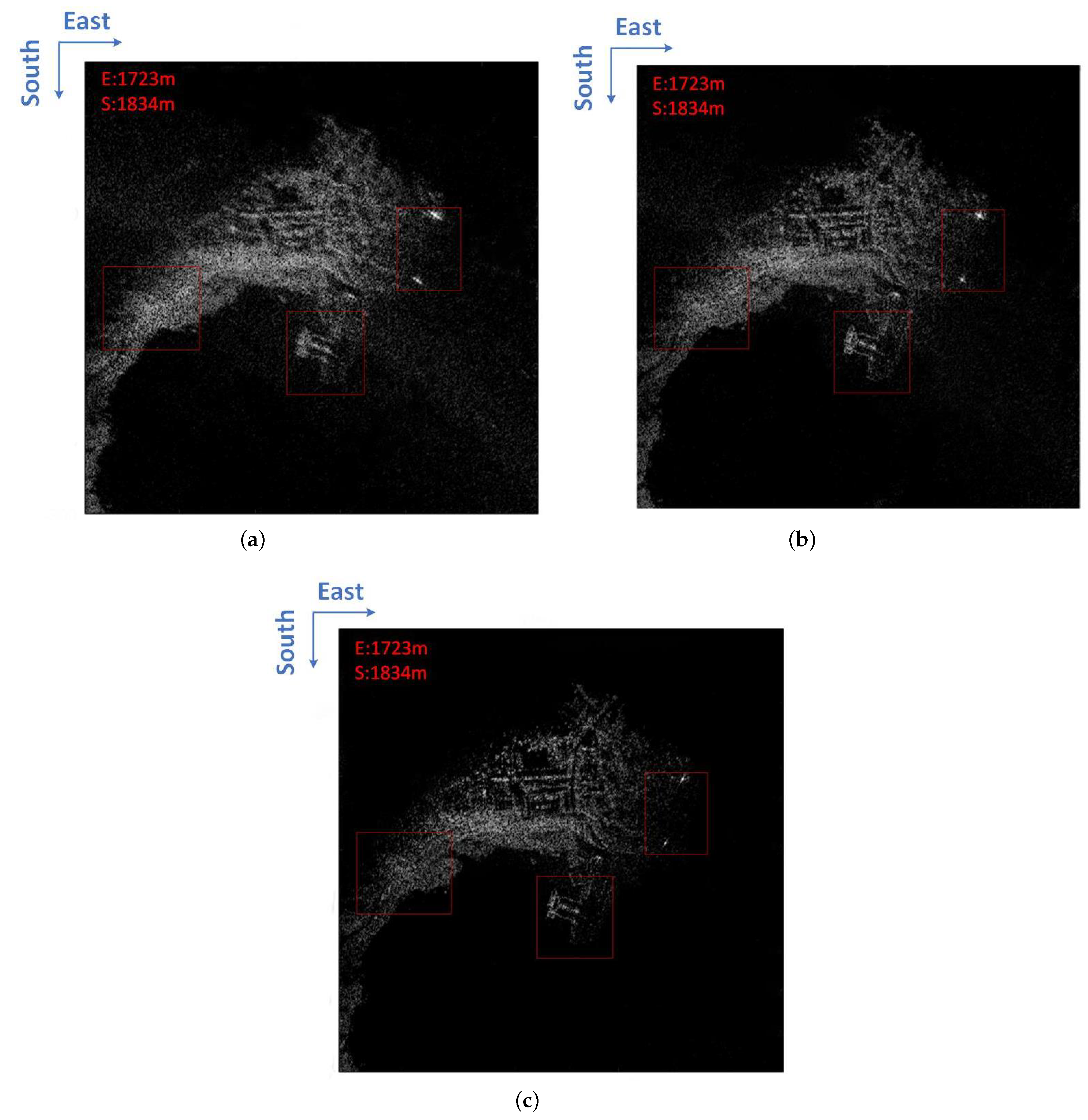
For imaging processing, first, the echo of transponders is used to realize time and frequency synchronization. Then, the NCS algorithm is used to get the coarse image as shown in Figure 13a. The imaging results have been corrected to the ground plane. It can be clearly seen that the whole scene is blurred and that the building outlines are indistinguishable. The false targets appear on both side of the strong points. Due to the short wavelength and unstable characteristics of the UAV platforms, even the second-order false target can be found. It is proved that high-frequency motion error has a large effect on the SAR image in mini-UAV-based BiSAR systems.

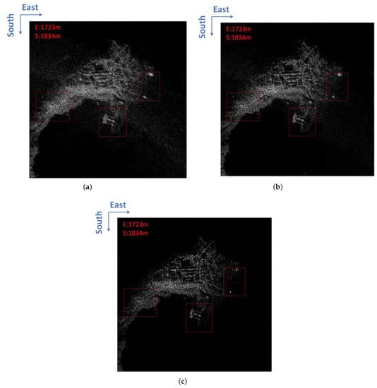
Figure 13. Image results of different MOCO algorithms. (a) is the image result without MOCO. (b) is the image result with traditional MOCO algorithm [11,23]. (c) is the result with proposed MOCO algorithm.

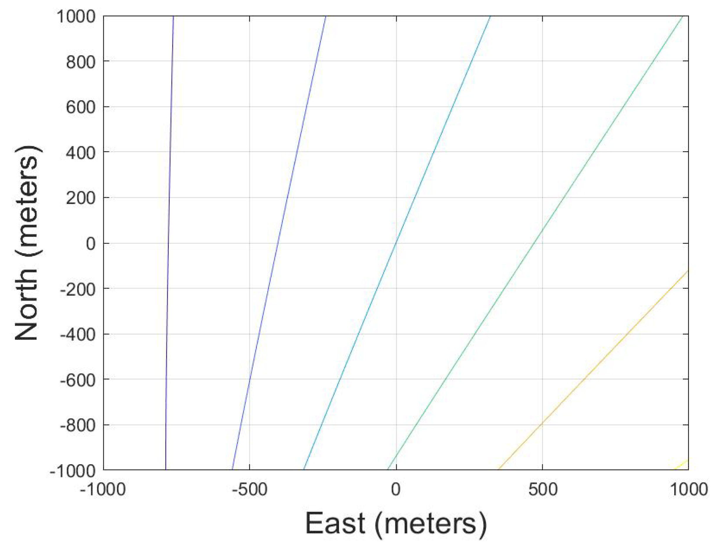
Then, the phase error is analyzed. Based on the error model shown in (6), it can be found that the error frequency component is only one through the azimuth phase. Next, traditional high-frequency MOCO algorithm [11] and the spatial variance compensation algorithm [23] are used. The spatial variance model is established along the range direction, which is shown in Figure 14. The line passing through the center of the scene is selected as the projection direction. The final compensation results are shown in Figure 13b. It can be found that the amplitude of the false targets has been decreased, but there are still false targets on both sides of the strong points. The whole image scene is also blurred. That means the spatial variance of the high-frequency is not well compensated. The estimation results of the amplitude and the initial phase of each subimage have deviations. This is because when the transmitter and receiver both affect the spatial variance, the spatial variance is so complex that it cannot be compensated by traditional spatial model. Furthermore, because the high-frequency motion error is not fully compensated, the bistatic low-frequency error compensation method [12] also has a deviation in the estimation of the Doppler parameters. Thus, the overall image is blurred.

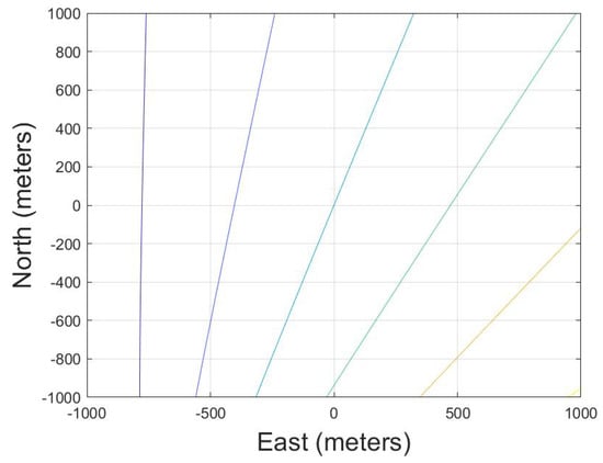
Figure 14. The range direction in the experiment configuration.

Next, the proposed MOCO algorithm is used. The approximate values of oscillation vectors are obtained through the INS. The position of the APC in the carrier coordinate system is shown in Table 5. The Euler angles are obtained from the INS whose maximum value and the initial phase are shown in Table 6. Next, combine the APC position with the platform rotation values; the approximate high-frequency motion error parameters are shown in Table 7.

Table 6. The error information obtained from the INS in the mini-UAV-based BiSAR experiment.

	Yaw Angle $\mathit{\alpha }$	Pitch Angle $\mathit{\beta }$	Roll Angle $\mathit{\theta }$	Initial Phase
Transmitter	${5.62}^{\circ }$	${7.18}^{\circ }$	${-3.52}^{\circ }$	$-{23.4}^{\circ }$
Receiver	${8.43}^{\circ }$	${-6.31}^{\circ }$	${5.72}^{\circ }$	${70.4}^{\circ }$

Table 7. High-frequency error parameters of the platforms obtained from the INS.

Platform	High-Frequency Error from the INS
	Amplitude H (mm)	Initial Phase ${\tilde{\mathit{\phi }}}_0\left({}^{\circ }\right)$
Transmitter	$\left[-2.4;-7.6;2.1\right]$	−23.4
Receiver	$\left[10.1;5.4;-3.0\right]$	70.4

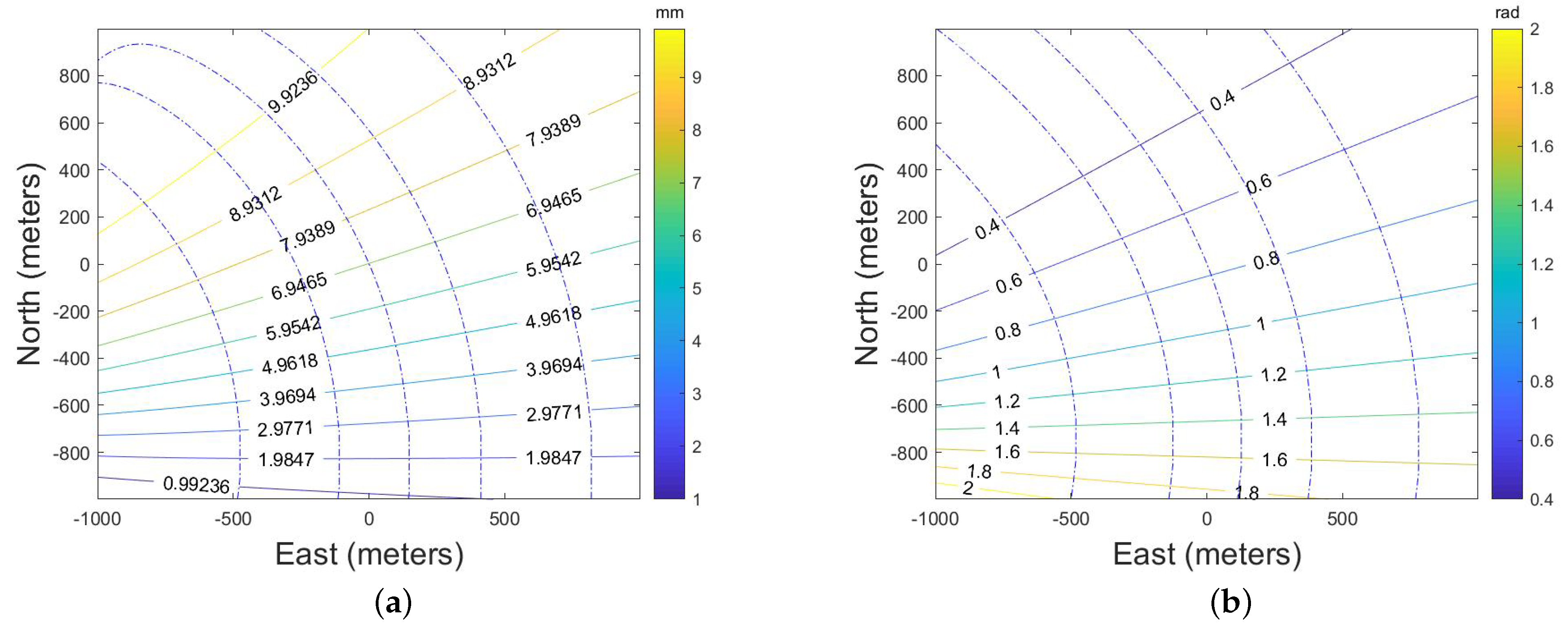
Based on the high-frequency error parameters, the gradient line of the amplitude and the initial phase can be obtained. The results are shown in Figure 15. Figure 15a is the gradient line of the amplitude. Figure 15b is the gradient line of the initial phase. The gradient line that passes through the center of the scene is chosen as the projection line. It can be seen that it is quite different from the projection line obtained by the traditional method. The final imaging result is shown in Figure 13c. It can be seen from the image result that the false target caused by the high-frequency error has been compensated. The transponders and other strong points are all well focused. At the same time, the details of the scene are more obvious, and the outlines of the hut and the wharf can be clearly identified. The result proves that the proposed MOCO algorithm can be used in a mini-UAV-based BiSAR system.

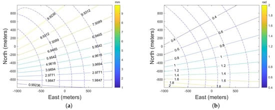
Figure 15. The bistatic spatial variance of the amplitude and initial phase under the BiSAR experiment. (a) is the result of amplitude. (b) is the result of the initial phase. The contour lines are shown as solid lines with values attached and the gradient lines are shown as blue dotted lines.

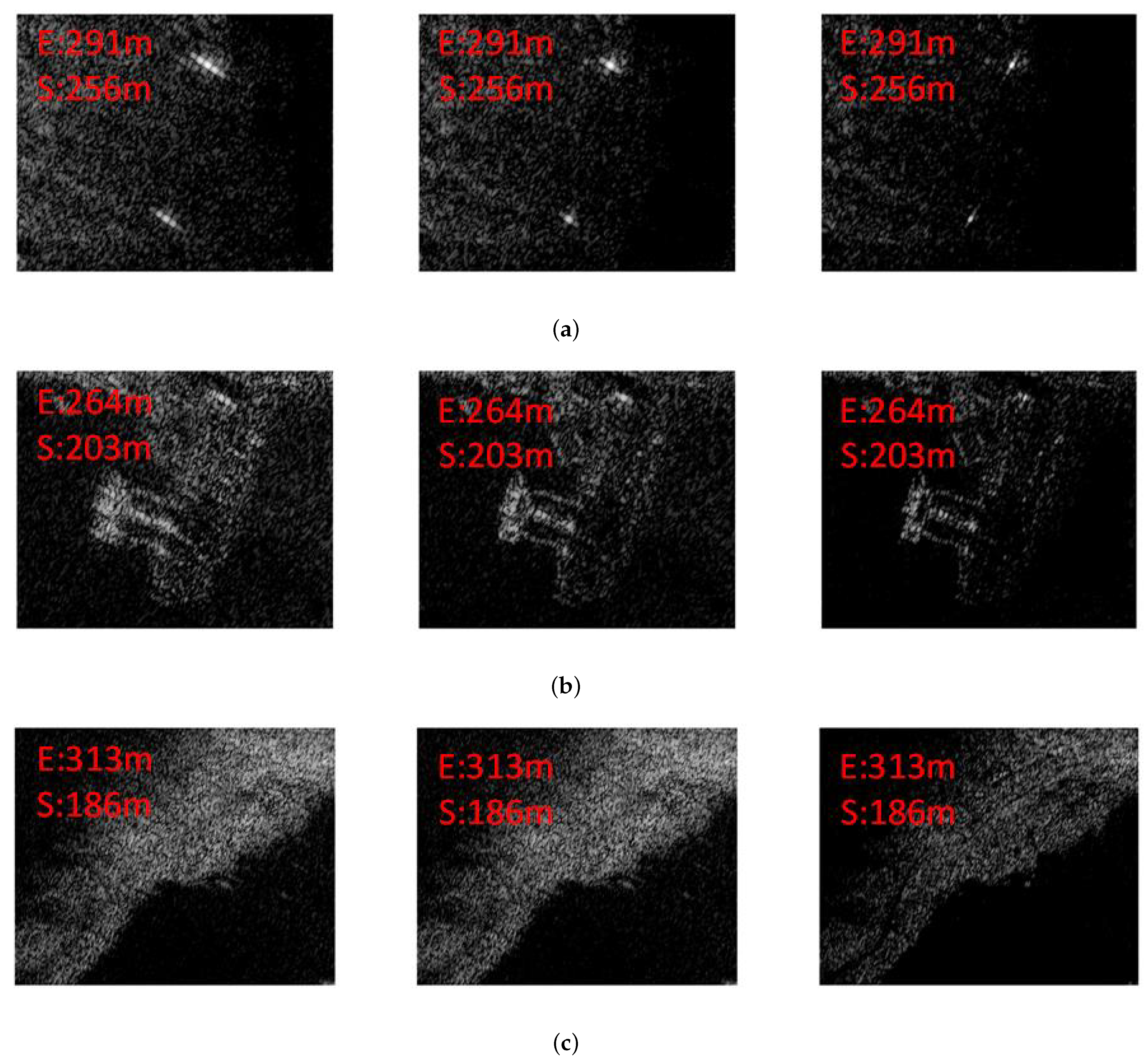
To further compare the results before and after the MOCO processing, the area framed in red in Figure 13 is enlarged. Figure 16a shows the results of two transponders, Figure 16b shows the result of the wharf, and Figure 16c shows the result of a road. From left to right are the image results without MOCO, with traditional MOCO algorithm [11,23], and with proposed MOCO algorithm. For the transponders, before high-frequency motion error compensation, the false targets around the transponders are large, and the second-order false targets can be found. In the second result, which is based on the traditional algorithm [11,23], the amplitude of the false targets are decreased but still can be found. Finally, in the third result, based on the proposed algorithm, the transponders are well focused. Furthermore, for the image scene, the outline of the wharf of the third image is much clearer than that of first two images. At the same time, only in the third one, the edge of the road can be found. It means that the proposed MOCO algorithm can effectively compensate the spatial variance of the high-monofrequency motion error in mini-UAV-based BiSAR systems.

Figure 16. Enlarged image results of different MOCO algorithms. (a) is the image result of two transponders. (b) is the image result of the wharf. (c) is the image result of a road. From left to right are the image results without MOCO, with traditional MOCO algorithm [11,23], and with proposed MOCO algorithm.

For a mini-UAV-based BiSAR system, the platforms are more susceptible to the external environment; the attitude of the aircraft will constantly change during the imaging process. Thus, the high-frequency motion error cannot be ignored. In a BiSAR system, the transmitter and receiver both introduce the motion error, when the frequency of the motion errors are similar, the errors will couple with each other and the spatial variance will be more complex. The traditional MOCO algorithm cannot compensate this error form as well as the bistatic spatial variance. The algorithm proposed in this paper can effectively deal with these problems and is suitable for mini-UAV-based BiSAR system.

4. Discussion

In mini-UAV-based BiSAR, high-frequency motion error cannot be ignored and both the transmitter and receiver will introduce the motion errors. The error parameters of high-frequency motion errors are $\left({\tilde{a}}_T,{\tilde{f}}_{eT},{\tilde{\phi }}_{0T}\right)$ and $\left({\tilde{a}}_R,{\tilde{f}}_{eR},{\tilde{\phi }}_{0\mathrm{R}}\right)$, respectively. When the error frequencies are different, i.e., ${\tilde{f}}_{eT}\ne {\tilde{f}}_{eR}$, (6) does not hold, and the high-frequency motion error of the system can be expressed as:

$$\Delta R_{high}\left(u,\mathbf{P}\right)=\sum _m{\tilde{a}}_{m}sin(2\pi {\tilde{f}}_{em}u+{\tilde{\phi }}_{0m})$$

(21)

where m is the number of the high-frequency motion error. It can be found that the high-frequency errors will not be coupled with each other such that all of the error parameters of each motion error components can be estimated. In this condition, the spatial variance of the motion error can be compensated separately through the trajectory estimation. The complex of the spatial variance is equal to that of the monostatic condition.

However, when the error frequencies are same, as shown in (6), the motion error are coupled with each other and the error parameters cannot be estimated. Furthermore, the spatial variance is more complex due to it being influenced by the transmitter and receiver at the same time. Thus, the spatial variance compensation algorithm proposed for monostatic SAR system cannot be used here. The proposed MOCO algorithm is necessary in a mini-UAV-based BiSAR condition.

5. Conclusions

In a mini-UAV-based BiSAR system, the high-frequency motion error cannot be ignored due to the fact that UAV platforms are more susceptible to the external environment. Furthermore, the transmitter and receiver will both introduce motion error such that there is more than one high-frequency error component. The high-frequency motion errors will be coupled with each other when the error frequencies are the same. In this condition, the spatial variance is more complex and the traditional compensation algorithm for monoSAR cannot be used here.

In this paper, an MOCO algorithm for high-monofrequency motion error in mini-UAV-based BiSAR systems is proposed. First, the rotation error model is re-established to describe the high-monofrequency error. Then, based on the error nonlinear gradient, the bistatic spatial variance can be modeled with a small deviation. Finally, the bistatic spatial variance can be adaptively compensated based on the error nonlinear gradient through the contour projection. Simulation and experimental data verify the effectiveness of the algorithm. This algorithm is suitable for high-monofrequency motion error compensation in BiSAR; the complex bistatic spatial variant can be solved through this algorithm.

References

- Sun, Z.; Wu, J.; Yang, J.; Huang, Y.; Li, C.; Li, D. Path Planning for GEO-UAV Bistatic SAR Using Constrained Adaptive Multiobjective Differential Evolution. IEEE Trans. Geosci. Remote Sens. 2016, 54, 6444–6457. [Google Scholar] [CrossRef]
- Lort, M.; Aguasca, A.; López-Martínez, C.; Marín, T.M. Initial Evaluation of SAR Capabilities in UAV Multicopter Platforms. IEEE J. Sel. Top. Appl. Earth Obs. Remote Sens. 2018, 11, 127–140. [Google Scholar] [CrossRef] [Green Version]
- Zhou, S.; Yang, L.; Zhao, L.; Bi, G. Quasi-Polar-Based FFBP Algorithm for Miniature UAV SAR Imaging Without Navigational Data. IEEE Trans. Geosci. Remote Sens. 2017, 55, 7053–7065. [Google Scholar] [CrossRef]
- Jiang, Y.; Wang, Z. Analysis for Resolution of Bistatic SAR Configuration with Geosynchronous Transmitter and UAV Receiver. Int. J. Antennas Propag. 2013, 2013, 245–253. [Google Scholar] [CrossRef] [Green Version]
- Zeng, T.; Wang, Z.; Liu, F.; Wang, C. An Improved Frequency-Domain Image Formation Algorithm for Mini-UAV-Based Forward-Looking Spotlight BiSAR Systems. Remote Sens. 2020, 12, 2680. [Google Scholar] [CrossRef]
- Zhang, M.; Wang, R.; Deng, Y.; Wu, L.; Zhang, Z.; Zhang, H.; Li, N.; Liu, Y.; Luo, X. A Synchronization Algorithm for Spaceborne/Stationary BiSAR Imaging Based on Contrast Optimization With Direct Signal From Radar Satellite. IEEE Trans. Geosci. Remote Sens. 2016, 54, 1977–1989. [Google Scholar] [CrossRef]
- Qiu, X.; Hu, D.; Ding, C. An Improved NLCS Algorithm With Capability Analysis for One-Stationary BiSAR. IEEE Trans. Geosci. Remote Sens. 2008, 46, 3179–3186. [Google Scholar] [CrossRef]
- Xiong, T.; Li, Y.; Li, Q.; Wu, K.; Zhang, L.; Zhang, Y.; Mao, S.; Han, L. Using an Equivalence-Based Approach to Derive 2-D Spectrum of BiSAR Data and Implementation Into an RDA Processor. IEEE Trans. Geosci. Remote Sens. 2021, 59, 4765–4774. [Google Scholar] [CrossRef]
- Lim, T.S.; Koo, V.C.; Ewe, H.T.; Chuah, H.T. High-frequency Phase Error Reduction in Sar Using Particle Swarm of Optimization Algorithm. J. Electromagn. Waves Appl. 2007, 21, 795–810. [Google Scholar] [CrossRef]
- Marechal, N. High frequency phase errors in SAR imagery and implications for autofocus. In Proceedings of the 1996 International Geoscience and Remote Sensing Symposium, Lincoln, NE, USA, 31 May 1996. [Google Scholar]
- Li, Y.; Wu, Q.; Wu, J.; Li, P.; Zheng, Q.; Ding, L. Estimation of High-Frequency Vibration Parameters for Terahertz SAR Imaging Based on FrFT With Combination of QML and RANSAC. IEEE Access 2021, 9, 5485–5496. [Google Scholar] [CrossRef]
- Wang, Z.; Liu, F.; Zeng, T.; Wang, C. A Novel Motion Compensation Algorithm Based on Motion Sensitivity Analysis for Mini-UAV-Based BiSAR System. IEEE Trans. Geosci. Remote Sens. 2021, 1–13. [Google Scholar] [CrossRef]
- Bao, M.; Zhou, S.; Yang, L.; Xing, M.; Zhao, L. Data-Driven Motion Compensation for Airborne Bistatic SAR Imagery Under Fast Factorized Back Projection Framework. IEEE J. Sel. Top. Appl. Earth Obs. Remote Sens. 2021, 14, 1728–1740. [Google Scholar] [CrossRef]
- Pu, W.; Wu, J.; Huang, Y.; Li, W.; Sun, Z.; Yang, J.; Yang, H. Motion Errors and Compensation for Bistatic Forward-Looking SAR With Cubic-Order Processing. IEEE Trans. Geosci. Remote Sens. 2016, 54, 6940–6957. [Google Scholar] [CrossRef]
- Miao, Y.; Wu, J.; Yang, J. Azimuth Migration-Corrected Phase Gradient Autofocus for Bistatic SAR Polar Format Imaging. IEEE Geosci. Remote Sens. Lett. 2021, 18, 697–701. [Google Scholar] [CrossRef]
- Li, D.; Lin, H.; Liu, H.; Wu, H.; Tan, X. Focus Improvement for Squint FMCW-SAR Data Using Modified Inverse Chirp-Z Transform Based on Spatial-Variant Linear Range Cell Migration Correction and Series Inversion. IEEE Sens. J. 2016, 16, 2564–2574. [Google Scholar] [CrossRef]
- Sun, Z.; Wu, J.; Li, Z.; Huang, Y.; Yang, J. Highly Squint SAR Data Focusing Based on Keystone Transform and Azimuth Extended Nonlinear Chirp Scaling. IEEE Geosci. Remote Sens. Lett. 2015, 12, 145–149. [Google Scholar] [CrossRef]
- Li, D.; Lin, H.; Liu, H.; Liao, G.; Tan, X. Focus Improvement for High-Resolution Highly Squinted SAR Imaging Based on 2-D Spatial-Variant Linear and Quadratic RCMs Correction and Azimuth-Dependent Doppler Equalization. IEEE J. Sel. Top. Appl. Earth Obs. Remote Sens. 2017, 10, 168–183. [Google Scholar] [CrossRef]
- Huang, L.; Qiu, X.; Hu, D.; Ding, C. Focusing of Medium-Earth-Orbit SAR With Advanced Nonlinear Chirp Scaling Algorithm. IEEE Trans. Geosci. Remote Sens. 2011, 49, 500–508. [Google Scholar] [CrossRef]
- Chen, J.; Zhang, J.; Jin, Y.; Yu, H.; Liang, B.; Yang, D.G. Real-Time Processing of Spaceborne SAR Data With Nonlinear Trajectory Based on Variable PRF. IEEE Trans. Geosci. Remote Sens. 2021, 1–12. [Google Scholar] [CrossRef]
- Prats-Iraola, P.; Scheiber, R.; Rodriguez-Cassola, M.; Mittermayer, J.; Wollstadt, S.; De Zan, F.; Bräutigam, B.; Schwerdt, M.; Reigber, A.; Moreira, A. On the Processing of Very High Resolution Spaceborne SAR Data. IEEE Trans. Geosci. Remote Sens. 2014, 52, 6003–6016. [Google Scholar] [CrossRef] [Green Version]
- Huang, D.; Guo, X.; Zhang, Z.; Yu, W.; Truong, T.K. Full-Aperture Azimuth Spatial-Variant Autofocus Based on Contrast Maximization for Highly Squinted Synthetic Aperture Radar. IEEE Trans. Geosci. Remote Sens. 2020, 58, 330–347. [Google Scholar] [CrossRef]
- Chen, J.; Xing, M.; Sun, G.C.; Li, Z. A 2-D Space-Variant Motion Estimation and Compensation Method for Ultrahigh-Resolution Airborne Stepped-Frequency SAR With Long Integration Time. IEEE Trans. Geosci. Remote Sens. 2017, 55, 6390–6401. [Google Scholar] [CrossRef]
- Tang, Y.; Zhang, B.; Xing, M.; Bao, Z.; Guo, L. The Space-Variant Phase-Error Matching Map-Drift Algorithm for Highly Squinted SAR. IEEE Geosci. Remote Sens. Lett. 2013, 10, 845–849. [Google Scholar] [CrossRef]
- Peng, B.; Wei, X.; Deng, B.; Chen, H.; Liu, Z.; Li, X. A Sinusoidal Frequency Modulation Fourier Transform for Radar-Based Vehicle Vibration Estimation. IEEE Trans. Instrum. Meas. 2014, 63, 2188–2199. [Google Scholar] [CrossRef]
- Wang, P.; Orlik, P.V.; Sadamoto, K.; Tsujita, W.; Gini, F. Parameter Estimation of Hybrid Sinusoidal FM-Polynomial Phase Signal. IEEE Signal Process. Lett. 2017, 24, 66–70. [Google Scholar] [CrossRef]
- Wang, Z.; Wang, Y.; Xu, L. Parameter Estimation of Hybrid Linear Frequency Modulation-Sinusoidal Frequency Modulation Signal. IEEE Signal Process. Lett. 2017, 24, 1238–1241. [Google Scholar] [CrossRef]
- Stankovic, L.; Dakovic, M.; Thayaparan, T.; POPOVIC-BUGARIN, V. Inverse radon transform–based micro-doppler analysis from a reduced set of observations. IEEE Trans. Aerosp. Electron. Syst. 2015, 51, 1155–1169. [Google Scholar] [CrossRef]
- Li, Z.; Wang, H.; Su, T.; Bao, Z. Generation of wide-swath and high-resolution SAR images from multichannel small spaceborne SAR systems. IEEE Geosci. Remote Sens. Lett. 2005, 2, 82–86. [Google Scholar] [CrossRef]
- Zhu, X.X.; Bamler, R. Very High Resolution Spaceborne SAR Tomography in Urban Environment. IEEE Trans. Geosci. Remote Sens. 2010, 48, 4296–4308. [Google Scholar] [CrossRef] [Green Version]
- Kong, Y.K.; Cho, B.L.; Kim, Y.S. Ambiguity-free Doppler centroid estimation technique for airborne SAR using the Radon transform. IEEE Trans. Geosci. Remote Sens. 2005, 43, 715–721. [Google Scholar] [CrossRef]
- Nies, H.; Loffeld, O.; Natroshvili, K. Analysis and Focusing of Bistatic Airborne SAR Data. IEEE Trans. Geosci. Remote Sens. 2007, 45, 3342–3349. [Google Scholar] [CrossRef]
- Xu, G.; Sugimoto, N. A linear algorithm for motion from three weak perspective images using Euler angles. IEEE Trans. Pattern Anal. Mach. Intell. 1999, 21, 54–57. [Google Scholar] [CrossRef]
- Fu, X.; Wang, B.; Xiang, M.; Jiang, S.; Sun, X. Residual RCM Correction for LFM-CW Mini-SAR System Based on Fast-Time Split-Band Signal Interferometry. IEEE Trans. Geosci. Remote Sens. 2019, 57, 4375–4387. [Google Scholar] [CrossRef]
- Sun, G.C.; Xing, M.; Wang, Y.; Yang, J.; Bao, Z. A 2-D Space-Variant Chirp Scaling Algorithm Based on the RCM Equalization and Subband Synthesis to Process Geosynchronous SAR Data. IEEE Trans. Geosci. Remote Sens. 2014, 52, 4868–4880. [Google Scholar] [CrossRef]
Publisher’s Note: MDPI stays neutral with regard to jurisdictional claims in published maps and institutional affiliations. |
© 2021 by the authors. Licensee MDPI, Basel, Switzerland. This article is an open access article distributed under the terms and conditions of the Creative Commons Attribution (CC BY) license (https://creativecommons.org/licenses/by/4.0/).