Integrating Normal Vector Features into an Atrous Convolution Residual Network for LiDAR Point Cloud Classification

Abstract

LiDAR point clouds are rich in spatial information and can effectively express the size, shape, position, and direction of objects; thus, they have the advantage of high spatial utilization. The point cloud focuses on describing the shape of the external surface of the object itself and will not store useless redundant information to describe the occupation. Therefore, point clouds have become the research focus of 3D data models and are widely used in large-scale scene reconstruction, virtual reality, digital elevation model production, and other fields. Since point clouds have various characteristics, such as disorder, density inconsistency, unstructuredness, and incomplete information, point cloud classification is still complex and challenging. To realize the semantic classification of LiDAR point clouds in complex scenarios, this paper proposes the integration of normal vector features into an atrous convolution residual network. Based on the RandLA-Net network structure, the proposed network integrates the atrous convolution into the residual module to extract global and local features of the point clouds. The atrous convolution can learn more valuable point cloud feature information by expanding the receptive field. Then, the point cloud normal vector is embedded in the local feature aggregation module of the RandLA-Net network to extract local semantic aggregation features. The improved local feature aggregation module can merge the deep features of the point cloud and mine the fine-grained information of the point cloud to improve the model’s segmentation ability in complex scenes. Finally, to resolve the imbalance of the distribution of the various categories of point clouds, the original loss function is optimized by adopting a reweighted method to prevent overfitting so that the network can focus on small target categories in the training process to effectively improve the classification performance. Through the experimental analysis of a Vaihingen (Germany) urban 3D semantic dataset from the ISPRS website, it is verified that the proposed algorithm has a strong generalization ability. The overall accuracy (OA) of the proposed algorithm on the Vaihingen urban 3D semantic dataset reached 97.9%, and the average reached 96.1%. Experiments show that the proposed algorithm fully exploits the semantic features of point clouds and effectively improves the accuracy of point cloud classification.

1. Introduction

With the rapid development of spaceborne, airborne, and terrestrial remote sensing, 3D data acquisition technologies are becoming increasingly mature, including various types of 3D laser scanners, depth cameras, and LiDAR technologies. The acquisition of point clouds is becoming more and more convenient, and the data volume of point clouds is increasing rapidly. Because of its rich geometry, shape, and scale information, point clouds play an important role in the understanding of three-dimensional scenes [1]. To describe the spatial information of point clouds at a deeper level, it is essential to classify point clouds. In many point cloud recognition tasks, point cloud classification has always been an active research field in photogrammetry and remote sensing. As a basic technology for point cloud data processing and analysis, it is widely used and plays a crucial role in automatic driving [2], smart urban areas [3], 3D reconstruction [4], forest monitoring [5], cultural heritage protection [6], power line detection [7], intelligent robots [8], and other fields. Point clouds have characteristics of large volume, disorder, and dispersion and uneven density distribution. Because of high sensor noise and complex three-dimensional scenes, there are many challenging problems associated with point cloud classification and semantic segmentation [9], which are current research hotspots.

Generally, point cloud classification and semantic segmentation are divided into two steps: the first is to extract representative point features, and the second is to use the learned features to divide each point into predefined semantic categories. Early studies mainly focused on manually extracting features and then using machine learning-based classifiers to predict the semantic label of each point, such as Gaussian mixture model [10], support vector machine (SVM) [11], AdaBoost [12], and random forest (RF) [13]. The traditional method of manual feature extraction relies too much on manual production and optimization methods, and the extraction efficiency is low; moreover, it can reduce classification accuracy because valuable information in the point cloud is lost and the relationship between adjacent points is ignored. Some researchers have attempted to resolve these problems by fusing context information, such as conditional random fields (CRF) [14] and Markov random field (MRF) [15,16], and these methods improve the classification performance to a certain extent. However, determining a method of selecting the optimal classifier for combination is relatively complex. Moreover, these methods are limited by the prior knowledge of scholars, and the generalization ability of the models is poor. Therefore, satisfactory results are not achieved when dealing with complex scenes, which limits the flexibility of these methods when applied to various real scenes. With the great success of deep learning in image feature extraction, an increasing number of neural network models (convolutional neural network [17,18], recursive neural network [19], deep belief network [20], etc.) continue to emerge and have achieved good results when dealing with practical application problems. Researchers are beginning to consider using deep learning to address point clouds. Because of the irregularity and inhomogeneous density of point clouds, traditional convolutional neural networks (CNN) cannot directly process the original unstructured point cloud. A few researchers have proposed an indirect learning point cloud feature extraction scheme based on deep convolutional neural networks. The point cloud is transformed into a regular structure suitable for convolutional neural network processing, such as multiview and voxel grid forms; however, these methods result in information loss and high spatial and temporal complexity. In 2016, Qi proposed the PointNet network [21], which directly learned unstructured original point clouds and made breakthroughs in object classification, semantic segmentation, and scene understanding.

RandLA-Net [22] uses random sampling to downsample the point cloud, which has the advantages of low time complexity and low space complexity. Inspired by RandLA-Net, this paper proposes the integration of normal vector features into an atrous convolution residual network for point cloud classification. The main contributions of this paper are summarized as follows.

1.

An atrous convolution is integrated into the residual structure. The atrous convolution can amplify the receptive field of the convolution layer without increasing the network parameters and can avoid the problem of feature loss caused by traditional methods, such as the pooling layer.

2.

The normal vector of the point cloud is embedded into the feature extraction module of the point cloud classification network, which improves the utilization of the spatial information of the point cloud and enables the network to fully capture the rich context information of the point cloud.

3.

A reweighted loss function is proposed to solve the problem of uneven distribution of point clouds, and it is an improved loss function based on the cross-entropy loss function.

4.

To verify the effectiveness of the proposed algorithm, we conducted experiments on the 3D semantic dataset of urban Vaihingen in Germany. The experimental results show that the proposed algorithm can effectively capture the geometric structure of 3D point clouds, realize the classification of LiDAR point clouds, and improve classification accuracy.

2. Related Work

2.1. Classification Based on Handcrafted Features

At present, traditional point cloud classification is mainly based on the point cloud color, curvature, intensity, echo frequency, and other characteristics, and it relies on the low-level features of the artificially designed point cloud. The existing traditional point cloud classification methods can be divided into two categories: one is to classify the point cloud based on geometric constraints, and the other is to classify the point cloud based on machine learning. In the point cloud classification method based on geometric constraints, it is usually necessary to set multiple constraints to distinguish each category. Zuo adopted a topological heuristic segmentation algorithm for object-oriented segmentation of raster elevation images. Based on the principle of maximum interclass variance, ground points and nonground points were separated and buildings and other ground objects were distinguished by multiple constraint conditions, such as the area and building height [23]. Brodu used three binary classifiers to classify vegetation, bedrock, sand and gravel, and water in natural scenes successively through three classifications [24]. In the point cloud classification method based on machine learning, Becker constructed multiple feature vectors and divided the point cloud into multiple scales by combining color information, then divided the point cloud into six categories by using RF [25]. Guo used JoinBoost to implement ground object classification and developed a serialized point cloud classification and feature dimensionality reduction method by combining the spatial correlation of ground objects, which decreased the dimension of the feature vector and reduced the classification time [26]. Niemeyer addressed the task of contextual classification of ALS point clouds by integrating an RF classifier into a CRF framework [27]. Subsequently, Niemeyer continued to expand this work and proposed a two-layer CRF to aggregate spatial and semantic context [28].

2.2. Classification Based on Deep Learning

With the emergence of deep learning, an increasing number of studies have been conducted on the application of deep learning to point cloud semantic segmentation, and great improvements have been achieved. In recent years, many researchers have introduced many point cloud segmentation models based on deep learning, which mainly include the following five categories.

2.2.1. Two-dimensional Multiview Method

Su first obtained 2D images of 3D objects from different perspectives, extracted features from each view, and aggregated images from different perspectives through a pooling layer and a full connection layer to acquire the final semantic segmentation result [29]. The 3D-Mininet proposed by Alonso obtained local and global context information from 3D data through multiview projection, and then input these data to a 2D full convolutional neural network (FCNN) to predict semantic labels. Finally, the predicted 2D semantic labels were reprojected into 3D space to obtain high-quality results in a faster and more efficient way [30].

2.2.2. Three-Dimensional Voxelization Method

Maturana advanced the VoxNet model, which is the first 3D CNN model based on voxel data and shows the potential of a 3D convolution operator to learn features from voxel-occupied grids; however, the sparsity of 3D data and incomplete spatial information lead to low efficiency of semantic segmentation [31]. In addition, Meng combined a variational autoencoder (VAE) to introduce VV-NET. After converting the point cloud into a voxel grid, each voxel was further subdivided into child voxels, and interpolation was carried out on the sparse point samples within the child voxels. The limitations of binary voxels were broken through by encoding and decoding, and the ability to capture point distribution was enhanced [32]. Hegde combined the voxelized network and the multiview network to propose the FusionNet model. The two networks are merged at the fully connected layer, and the performance is significantly improved compared with that of the single network [33].

2.2.3. Neighborhood Feature Learning

Qi developed PointNet [21], which pioneered feature learning directly on the unstructured original point cloud. Although PointNet showed good performance in point cloud classification and semantic segmentation, it failed to capture the local structure features caused by metric space points, thus limiting the ability of fine-grained pattern recognition and complex scene generalization. Therefore, the author advanced an improved version based on PointNet, i.e., PointNet ++, in which each layer has three substages: sampling, grouping, and feature extraction. This network not only resolves the problem of uneven sampling of point cloud data but also considers the distance measurement between points [34]. To realize direction perception and scale perception at the same time, Jiang proposed the PointSift module based on the PointNet network, which integrated information from eight directions by direction-encoding convolution (OEC) to obtain the representation of encoding orientation information and realized multiscale representation by stacking multi-direction encoding units [35]. Zhao introduced a PointWeb network, which built a local fully connected network by inserting an adaptive feature adjustment (AFA) module, learned point feature vectors from point-pair differences, and realized adaptive adjustment [36].

2.2.4. Graph Convolution

Wang advanced a local spectral convolution, which constructs a local graph from the neighborhood of a point and uses spectral convolution combined with a new graph pool strategy to learn the relative layout and features of adjacent points [37]. Loic introduced the super-point graph (SPG), which is based on a gated graph neural network and edge conditional convolution (ECC), to obtain context information and showed that it performs well in large-scale point cloud segmentation [38].

2.2.5. Optimizing CNN

Li developed PointCNN, which converts a disordered point cloud into a corresponding canonical order by learning the X-transform convolution operator and then uses the CNN architecture to extract local features [39]. Xu developed SpiderCNN, which extends the convolution operation from the conventional grid to the irregular point set. At the same time, a step function is constructed to encode the spatial geometric information in the local neighborhood and extract the deep semantic information [40].

3. Materials and Methods

To enhance a network’s ability to extract the fine-grained features of the local region and the deep semantic information of the point cloud, this paper proposes the integration of normal vector features into an atrous convolution residual network. We propose a fusion atrous convolution residual block, which fuses the atrous convolution into the residual structure of the network. To ensure the receptive field of the convolution block, the characteristics of the ordinary convolution block and the atrous convolution block are fully utilized. The network’s ability to capture the local geometric features of the point cloud is enhanced, and higher semantic information of the point cloud is learned. At the same time, the normal vector of the point cloud is integrated with the local feature aggregation module in the network, which fully exploits the characteristics of the point cloud, improves the utilization rate of the spatial information of the point cloud, and enhances the recognition network’s ability to ground objects. We also propose an improved loss function to resolve the uneven distribution of each category.

The proposed network adopts a widely used encoder–decoder architecture with skip connections. The proposed network structure is shown in Figure 1. The input point cloud is fed to a shared MLP layer to extract the features of each point, and then five encoding and decoding layers are used to learn the features of each point. Finally, a fully connected layer is applied to predict the semantic label of each point cloud. Five encoding layers are used to progressively reduce the size of the point clouds and increase the per-point feature dimensions, and five decoding layers are used after five encoding layers. The point cloud is downsampled with a 4-fold decimation ratio. In addition, the dimension of each point feature is increased to retain more information. Each encoding layer contains a fusion residual atrous convolution (FACR) module as the point cloud of the local and global feature extraction modules. For each layer in the decoder, the KNN algorithm is used to find the nearest neighbor of each point, and then the feature set of points is upsampled by nearest-neighbor interpolation. Then, the updated sampling features are connected with the intermediate features generated by the encoding layer by using the skip connection, and the connected features are input into the shared MLP layer. The network output is the semantic prediction label of each point, expressed as $N\times n$, where $N$ is the number of input point clouds and $n$ is the number of categories of the input point clouds.

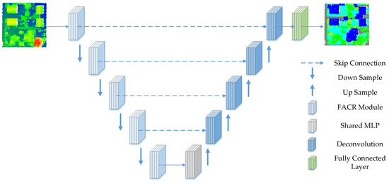
Figure 1. The framework of the proposed integrating normal vector features into an atrous convolution residual network. The input point clouds on the left are colored by elevation, and the output is the classification result.

3.1. FACR (Fusion Atrous Convolution Residual) Module

Compared with shallow neural networks, deep networks can achieve more abstract point cloud feature extraction due to their high-dimensional nonlinear operations. However, when the network increases to a certain depth, the weights of the hidden layers in the front part are slowly updated or stagnant, resulting in saturation of the classification accuracy. If the network continues to deepen, the accuracy will decline rapidly. Given this problem, He in 2015 introduced a residual network structure based on skip connections [41], which can effectively solve the gradient descent caused by the increase in network depth. In addition, the mapping after the introduction of residual blocks is more sensitive to the change in output and has a greater effect on the adjustment of weight; therefore, the network segmentation effect is better. The network architecture mentioned in this article mainly includes a significant structure to extract the geometric structure features and semantic features of the point cloud—namely, the FACR module. If the ordinary convolution in the residual block is replaced by the atrous convolution, the depth of the network is reduced and some expression ability of the original network is lost, although the characteristics of each level are improved and the size of the receptive field is expanded. Therefore, by integrating the atrous convolution into the residual structure, more point cloud characteristic information can be extracted, which ensures high accuracy and reduces the number of parameters and computation. Because the point cloud will be subsampled at each encoding layer, some point clouds will be discarded. To retain and utilize the geometric details and spatial features of the input point cloud as much as possible, an atrous convolution residual module is proposed for local feature extraction. In the encoding phase, the normal vector of the point cloud is introduced to embed the normal vector into the local feature attention module to extract more feature information. Two local feature attention modules are connected and stacked with atrous convolution and a skip connection layer, and a residual block is ultimately formed. As shown in Figure 2, the module is mainly composed of four neural units: shared MLP, local feature block, attention pooling, and atrous convolution. In the following, the local feature attention (LFA) module is introduced in detail, as shown in Figure 3.

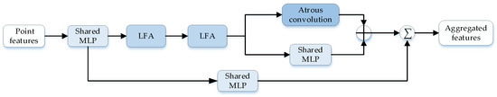
Figure 2. Fusion atrous convolution residual module.

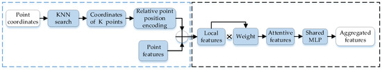
Figure 3. Local feature attentive module (LFA).

In Figure 3, the content in the blue dotted box on the left is defined as a local feature block. Given the point cloud P and its features, to improve the calculation efficiency, the KNN algorithm based on the Euclidean distance of the point is used to search K adjacent points of point P and obtain the 3D coordinates and normal vectors of the neighborhood point set. Then, the spatial position coding of this point P is calculated. The coding content includes the three-dimensional coordinates of point cloud P, the three-dimensional coordinates of neighboring points, the normal vector of neighboring points, the relative coordinates between P and neighboring points, and the Euclidean distance between P and neighboring points, as shown in Equation (1). The result of spatial position coding is cascaded with the point cloud feature to obtain the enhanced feature of point P, as shown in Equation (2). This module ensures that the features of point P always grasp the relative spatial position between them so that the network can learn the complex local structure of the point cloud more effectively, enabling the network to extract the local neighborhood feature information and the context relationship between point P and the neighboring points more deeply.

$$r_i^k=MLP\left(p_i\oplus p_i^k\oplus n{p}_i^k\oplus \left(p_i-p_i^k\right)\oplus \Vert p_i-p_i^k\Vert \right)$$

(1)

where $p_i$ is the three-dimensional coordinate of point P, $p_i^k$ is the coordinate of one of the K adjacent points, $n{p}_i^k$ is the normal vector of one of the K adjacent points, $\oplus$ represents the concatenation operation, and $r_i^k$ is the spatial position coding of point P.

$${\widehat{f}}_i^k=f_i^k\oplus r_i^k$$

(2)

where $r_i^k$ represents the spatial position coding of point P, $f_i^k$ is the original or generated feature of point P, ${\hat{f}}_i^k$ is the enhanced feature after concatenation, and $\oplus$ represents the concatenation operation.

The content in the black dashed box on the right in Figure 3 is defined as the attention pooling module. Existing neural networks usually use maximum pooling or average pooling methods to extract features, although they will cause the loss of some useful information. Attention pooling can learn more critical features from a large number of input features, can reduce the attention of unimportant features, and can even filter out the interference of some irrelevant features. In general, the aggregation of features can be optimized by attention pooling. Therefore, this paper adopts attention pooling to automatically select important local features. The attention pooling module calculates the weights of the local features gained from the local feature blocks, retains useful local features, and finally obtains aggregated features. For the set of enhanced features obtained from local feature blocks, the attention pooling module first performs a full join operation to integrate the feature representations. Then, the attention score is acquired through the softmax function. Through the attention score, the essential features with high scores are selected. Finally, these features are aggregated after weighted summation. At the beginning of network training, the attention pooling module tends to select prominent keypoint features, and after a large subsampling of the point cloud, the attention pooling module is more inclined to retain the main part of the point cloud features.

First, the score for each feature is calculated as a mask. Based on a set of local enhancement features $\widehat{F_i}=\left\{{\widehat{f}}_i^1\dots {\widehat{f}}_i^k\dots {\widehat{f}}_i^K\right\}$, a g () function is defined to learn the attention score for each feature, which consists of a multilayer perceptron (MLP). The learned attention score can be used as a mask to automatically select important features. W is the learning weight of the MLP, and the mask is shown in Equation (3):

$$s_i^k=g\left({\widehat{f}}_i^k,W\right)$$

(3)

where $s_i^k$ is the mask, which is used to remove the unimportant features. As shown in Equation (4), the weighted sum of the local feature and the corresponding attention score is used to obtain the local aggregate feature ${\tilde{f}}_i$.

$${\tilde{f}}_i={\displaystyle \sum }_{\mathrm{k}=1}^{\mathrm{K}}\left({\widehat{f}}_i^k\cdot s_i^k\right)$$

(4)

3.2. Normal Vector Calculation of the Point Cloud

The normal vector is one of the important attributes of the point cloud. There are three methods for solving the normal vector of the point cloud: the Delaunay triangulation method, the robust statistical method, and the local surface fitting method. The method in this paper is based on the local surface fitting method, which is widely used in large-scale point cloud scenarios with simple calculation principles and high efficiency.

Combined with the least squares principle, the normal vector of each point is estimated by fitting the K neighborhood points of each point. When the point clouds are dense and the search radius is small, the normal vector of each point can be expressed by the normal vector of the local fitting plane. Therefore, according to the least squares principle, the K neighborhood points of each point are fitted into a plane, and the calculation formula is shown in Equation (5):

$$p(n,d)=\mathrm{argmin}{\displaystyle \sum _{i=1}^k{\left(n{p}_i-d\right)}^2}$$

(5)

where $n$ is the normal vector of the local fitting plane $p$, and $d$ is the distance between the fitting plane $p$ and the coordinate origin. Principal component analysis is used to analyze the eigenvector corresponding to the minimum eigenvalue of the covariance matrix $A$—that is, the normal vector of the plane $p$. The formula of the covariance matrix $A$ is shown in Equation (6):

$$A={{\displaystyle \sum _{i=1}^k(pi-\overline{p})}}^{\mathrm{T}}(pi-\overline{p})$$

(6)

where $\overline{p}$ represents the center of mass of $K$ neighborhood points.

The fitting plane $p$ satisfies the condition that the sum of squares of the distances between adjacent points and the plane is the minimum. According to the Lagrange theorem, the covariance matrix $A$ and the plane normal vector $\overrightarrow{n}$ satisfy the following relationship:

$$A\overrightarrow{n}=\lambda \overrightarrow{n}$$

(7)

where $\lambda$ is the eigenvalue of $A$. When $\lambda$ is the minimum value, the corresponding vector $\overrightarrow{n}$ is the normal vector of the fitting plane $p$—that is, the normal vector of the point $pi$.

3.3. Atrous Convolution

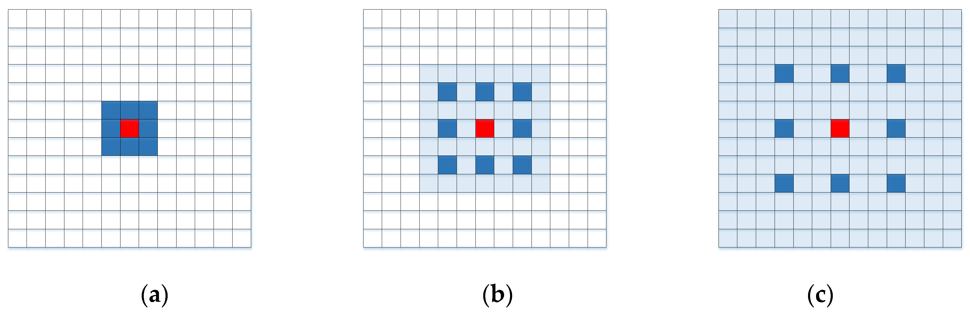
Atrous convolution [42] is a kind of convolution with a special structure that introduces the concept of dilatancy based on ordinary convolution. It has the function of expanding the convolution kernel receptive field. By setting different dilation rates, the multiscale feature information of the point cloud can be captured. Atrous convolution expands the scope of the convolution kernel. Atrous convolution with different dilation rates is shown in Figure 4, where panel (a) corresponds to the convolution of dilation rate 1, and the atrous convolution is equivalent to the standard convolution, i.e., the traditional $3\times 3$ convolution kernel, and the receptive field is $3\times 3$; panel (b) corresponds to the convolution with a dilation rate of 2, although the size of the convolution kernel is still $3\times 3$, while the receptive field increases to $7\times 7$; and panel (c) corresponds to the convolution with a dilation rate of 3, and its receptive field is $13\times 13$. The size of the receptive field increases with the dilation rate, although the number of parameters in Figure 4a–c does not increase. Therefore, more information can be obtained by replacing the traditional convolution kernel with the atrous convolution kernel without increasing the amount of calculation.

Figure 4. Atrous convolution with different dilation rates. (a) $\mathrm{r}=1$; (b) $\mathrm{r}=2$; (c) $\mathrm{r}=3$.

In this paper, atrous convolution is introduced into the residual block to expand the receptive field of features and capture richer contextual information without increasing network parameters and losing point cloud resolution. For the design of the dilation rate in the network model, the optimal dilation rate is determined by ablation experiments, which are described in Section 4. The size of the atrous convolution kernel and receptive field is defined by Equations (8) and (9), respectively:

$$f_n=f_k+(f_k-1)\times (D_r-1)$$

(8)

$$l_m=l_{m-1}+\left[(f_n-1)\times {\displaystyle \prod _{i=1}^{m-1}{S}_i}\right]$$

(9)

where $f_k$ is the representation of the size of the original convolution kernel; $f_n$ represents the size of the atrous convolution kernel; $D_r$ denotes a dilation rate; $l_{m-1}$ represents (m−1) layer receptive field size; $l_m$ represents the size of receptive field in the m-th layer after atrous convolution; and $S_i$ represents the stride size of layer i.

3.4. Reweighted Loss Function

By reweighting the cross-entropy loss function, the proportion of the classification loss in the total loss of the small target point cloud can be increased. At the same time, the proportion of the classification loss function of the large target point cloud in the total loss function is reduced so that the network can pay more attention to the small target category in the training process. Thus, it counteracts in reverse the overfitting problem of large target point clouds caused by unbalanced class distributions in neural network learning. This paper introduces reweighting to optimize the original loss function, using two different weight calculation methods to obtain two kinds of weights. The two kinds of weights are combined linearly, and then the new weight value is used to weight the loss function.

Generally, the general formula for reweighting the cross-entropy loss function is as follows:

$$L_{ce}=weight\cdot (-\ln (\frac{\exp (z_j)}{{\displaystyle \sum _{i=1}^N\exp (z_i)}}))$$

(10)

Suppose that the neural network input is the point cloud X, where N is the length of the output vector of the last layer of the network—that is, the number of categories in the point cloud. $z_j$ and $z_i$ are the j and i values of the output vector, $weight$ is the weight of reweighting the loss function, and the length of the weight vector is equal to N. The weight value of each type of loss is set according to the proportion of the point cloud in the data of this category. The category with too many samples is given a small weight, while the category with too many samples is given a large weight. Therefore, according to the principle of reweighting, this paper advances the first weight setting method as follows:

$$a_i=\frac{1}{\ln (\frac{N_i}{{\displaystyle \sum _{j=1}^n{N}_j}}+1.2)}$$

(11)

where $N_i$ is the number of point clouds of class i in the data, $a_i$ is the weight value of the point clouds of class i, and n is the number of categories. Although it is necessary to give a large weight to the category with a small number of point clouds, the weight should not be too large; otherwise, the neural network will also tend to the category with a large weight during training. From the monotonic nature of the ln(X) function, when the base n is greater than 1, the function is a monotonically increasing function. As the X value increases, the function tends to flatten out. Therefore, the ln(X) function is used to calculate the weight value. The second weight calculation method is obtained through the definition of the effective sample number, and the specific inference process is provided in the literature [43]. The calculation formula of the weight is as follows:

$$b_i=\frac{1-\Omega }{(1-{\Omega }^{n_i})}$$

(12)

where $b_i$ is the weight value of the class i sample, and $n_i$ is the sample number of the class i sample. According to the literature [41], the parameter Ω is equal to 0.99. The weight obtained by Equation (11) is calculated by using the proportion of each type of sample in the total number of samples. The calculation method is simple and can effectively improve the accuracy of the model, but the robustness is not strong. The weight $b_i$ obtained in Equation (12) is calculated by the number of effective samples, which can better reverse the overfitting problem of a large target point cloud in model training, and the robustness of the model is better when using this weight. The two weighting methods have their advantages and disadvantages; therefore, the two weights are combined linearly. The improved cross-entropy loss function is as follows:

$$L_{ce}=(a+b)\cdot (-\ln (\frac{\exp (z_j)}{{\displaystyle \sum _{i=1}^N\exp (z_i)}}))$$

(13)

4. Experimental Results and Analysis

4.1. Experimental Data

The experimental dataset is the Vaihingen (Germany) urban 3D semantic dataset (http://www2.isprs.org/commissions/comm3/wg4/3d-semantic-labeling.html, accessed on 12 October 2020), and it is provided by the International Society for Photogrammetry and Remote Sensing (ISPRS). The dataset includes airborne LiDAR point clouds covering three independent areas of urban Vaihingen. The data were collected in August 2008 and have an average altitude of approximately 500 meters and a field of view of 45 degrees. The average point density is approximately 8 per square meter, which is scanned by a LeicaALS50 airborne lidar system. The dataset contains a rich geographical environment, urban environment, and building types, which can fully verify the application of the algorithm in outdoor complex scenes. The dataset contains nine types of features: building roofs, trees, low vegetation, powerlines, shrubs, fences, impervious surfaces, building facades, and cars.

According to the standard setting of the ISPRS 3D label competition, the whole dataset is divided into two parts. The first scene (left in Figure 5) has 753,876 points as the training dataset, and the other two scenes (right in Figure 5) have 411,722 points as the test dataset. The details of each scene are shown in Table 1. Each scene is provided by an ASCII file with 3D coordinates, reflectivity, return count information, and point labels.

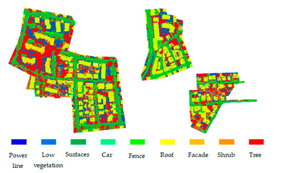
Figure 5. Vaihingen (Germany) urban 3D semantic dataset.

Table 1. Number of points in each object category of the training and test datasets.

Categories	Train	Test
Powerline	546	600
Low vegetation	180,850	98,690
Impervious surfaces	193,723	101,986
Car	4614	3708
Fence/Hedge	12,070	7422
Roof	152,045	109,048
Facade	27,250	11,224
Shrub	47,605	24,818
Tree	135,173	54,226

4.2. Experimental Setup

The experimental environment of the proposed algorithm in the data training and testing process is based on the Windows 10 system, Intel(R)Core (TM) i7 -10700 CPU, 64 GB memory, NVIDIA GeForce RTX 2080 Ti GPU, and the deep learning framework is TensorFlow-1.11.0. In this experiment, the Adam optimizer was used to train the network; the initial learning rate was 0.01, the retention rate of the dropout parameter of the fully connected layer was 0.5, and the Xavier optimizer initialized the network parameters.

4.3. Classification Performance Evaluation

To evaluate the performance of the point cloud classification algorithm, we usually need an objective evaluation index to ensure the fairness of the algorithm. In this paper, the overall accuracy ($OA$), $F1$ value, average $F1$ value, $recall$ and $precision$ are used to evaluate the test results. The overall accuracy measures the classification accuracy of all categories as a whole, and the $F1$ value deals with each category separately while considering $recall$ and $precision$. It is expressed by Equations (14)–(17).

$$OA=\frac{TP+TN}{TP+TN+FP+FN}$$

(14)

$$precision=\frac{TP}{TP+FP}$$

(15)

$$recall=\frac{TP}{TP+FN}$$

(16)

$$F1=2\ast \frac{precision\ast recall}{precision+recall}$$

(17)

where TP indicates the number of points that were in the original class i and correctly predicted as class i; TN represents the number of points that were in the original class j and predicted to be class j; FP indicates the number of points that were in the original class i but incorrectly predicted as class j; and FN represents the number of points that were in the original class j and predicted to be class i.

4.4. Experiments and the Analysis

The influence of embedding a normal vector into a feature extraction module, fusing an atrous convolution residual module and an improved loss function on the accuracy of point cloud classification, are discussed. The final result of the point cloud classification of the Vaihingen urban 3D semantic dataset is shown in Figure 6. From Figure 7, when the normal vector is not embedded and the atrous convolution residual module is not fused, the result of classification error by using the original loss function is obvious, especially in the areas of building roofs, low vegetation, and trees. The neural network adopts a normal vector model and atrous convolution residual model. Therefore, it can focus the local point cloud features and enrich the fusion features. The improved loss function emphasizes the small target point cloud with fewer point clouds, and the misclassification phenomenon is effectively suppressed. These findings suggest that the effectiveness of the proposed algorithm in cloud classification of complex scenarios.

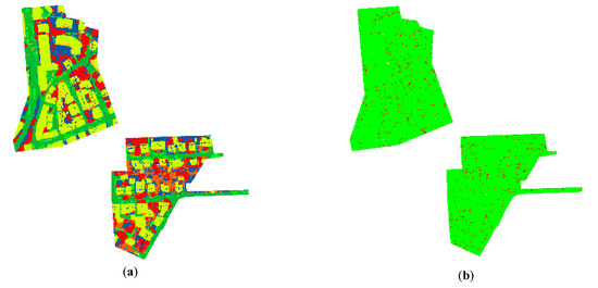
Figure 6. (a) Classification results of the Vaihingen urban 3D semantic dataset; (b) error map.

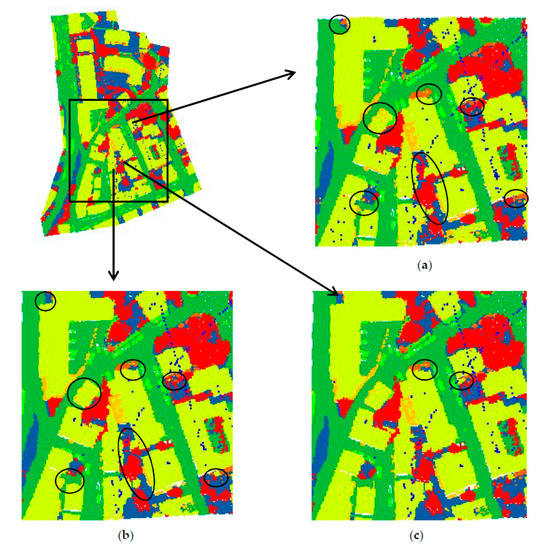
Figure 7. Classification results of the Vaihingen urban 3D semantic dataset obtained by different algorithms, where the black circle highlights the differences among (a–c). (a) Baseline; (b) Ours; (c) Ground truth.

4.4.1. Comparison and Analysis with the ISPRS Competition Method

To verify the effectiveness and superiority of the proposed algorithm in the point cloud classification of outdoor 3D scenes, it is compared with other advanced methods. The ISPRS website provides experimental results of different methods. Table 2 lists the OA value and the F1 value of the algorithm in this paper and these comparison methods. NANJ2, WhuY3, and WhuY4 are all point cloud classifications based on the point cloud feature map. WhuY3 is based on a single-scale point cloud feature map, while NANJ2 and WhuY4 are founded on a multiscale point cloud feature map. As shown in Table 2, compared with WhuY2 and WhuY3, which use a point cloud feature map for segmentation, the algorithm in this paper directly segments the point cloud. Considering the deep features among the point cloud features, the segmentation accuracy is improved. The F1 value of the proposed algorithm reached 96.1%, which is 26.9% higher than that of the most advanced WhuY4 model. The FACR module introduced in this paper can better extract point features. In addition, our model obtains 97.9% of the OA value, which is 12.7% higher than the most advanced NANJ2 model. Moreover, the NANJ2 algorithm uses RGB, strength, roughness, and other features as input for point cloud classification, while the algorithm in this paper only uses the original XYZ coordinate and normal vector as input. The algorithm in this paper has achieved higher accuracy in most categories.

Table 2. Comparison of the proposed method in this paper with the results provided by the ISPR website.

F1 Score
Method	Power Line	Low Vegetation	Surfaces	Car	Fence	Roof	Facade	Shrub	Tree	OA	Average F1
UM	0.461	0.790	0.891	0.477	0.052	0.920	0.527	0.409	0.779	0.808	0.590
WhuY2	0.319	0.800	0.889	0.408	0.245	0.931	0.494	0.411	0.773	0.810	0.586
WhuY3	0.371	0.814	0.901	0.634	0.239	0.934	0.475	0.399	0.780	0.823	0.616
LUH	0.596	0.775	0.911	0.731	0.340	0.942	0.563	0.466	0.831	0.816	0.684
BIJ_W	0.138	0.785	0.905	0.564	0.363	0.922	0.532	0.433	0.784	0.815	0.603
RIT_1	0.375	0.779	0.915	0.734	0.180	0.940	0.493	0.459	0.825	0.816	0.633
NANJ2	0.620	0.888	0.912	0.667	0.407	0.936	0.426	0.559	0.826	0.852	0.693
WhuY4	0.425	0.827	0.914	0.747	0.537	0.943	0.531	0.479	0.828	0.849	0.692
Ours	0.938	0.975	0. 990	0.982	0.946	0.992	0.917	0.930	0.977	0.979	0.961

4.4.2. Comparison with Other Deep Learning Classification Methods

In a comparative analysis with other deep learning methods, we counted the validation results on the 3D semantic dataset of urban Vaihingen in Germany, as shown in Table 3. Compared with other deep learning algorithms (PointNet [21], PointNet++ [34], PointnetSIFT [35], PointnetCNN [39], D-FCN [44], KPConv [45], GADH-Net [46]), the algorithm in this paper can obtain better feature expression. The FACR module can mine fine-grained local features with greater discriminative ability. The improved reweighted cross-entropy loss function can improve the segmentation accuracy of small object punctuation clouds. Compared with the most advanced GADH-Net, the OA value has increased by 12.9%, and the average F1 value has increased by 24.4%. Because the scene of the Vaihingen urban 3D semantic dataset includes messy information and many semantic categories of the point cloud, it is more challenging to classify the point cloud.

Table 3. Comparison of the proposed algorithm and deep learning algorithm.

F1 Score
Method	Power line	Low vegetation	Surfaces	Car	Fence	Roof	Facade	Shrub	Tree	F1	Average F1
PointNet	0.526	0.700	0.832	0.112	0.075	0.748	0.078	0.246	0.454	0.657	0.419
PointNet++	0.579	0.796	0.906	0.661	0.315	0.916	0.543	0.416	0.770	0.812	0.656
PointnetSIFT	0.557	0.807	0.909	0.778	0.305	0.925	0.059	0.444	0.796	0.822	0.677
PointnetCNN	0.615	0.827	0.918	0.758	0.359	0.927	0.578	0.491	0.781	0.833	0.695
D-FCN	0.704	0.802	0.914	0.781	0.370	0.930	0.605	0.460	0.794	0.822	0.707
KPConv	0.631	0.823	0.914	0.725	0.252	0.944	0.603	0.449	0.812	0.837	0.684
GADH-Net	0.668	0.668	0.915	0.915	0.350	0.946	0.633	0.498	0.839	0.850	0.717
Ours	0.938	0.975	0. 990	0.982	0.946	0.992	0.917	0.930	0.977	0.979	0.961

In Table 3, a comparison of the classification indexes of different ground objects shows that the algorithm proposed in this paper has a better segmentation effect on five kinds of features—namely, building roofs, low vegetation, surfaces, cars, and trees—and that these results are better than for other kinds of features. The F1 values of these five features are all above 97%, and the F1 value of the building roof is 99.2%, mainly because of the five features themselves. The normal vectors of building roofs, low vegetation, surfaces, and trees have high-resolution capabilities. Therefore, the proposed algorithm extracts deeper features, which further improves the network’s ability to recognize the five features. The algorithm in this paper has a poor segmentation effect on shrubs and building facades, mainly because of the limited training data available for shrubs and building facades. The network presents difficulty distinguishing the deep features of shrubs and building facades from other ground features. Although the training data of power lines and cars have fewer points, they show completely different characteristics from the other categories, thus obtaining higher classification performance. The experimental results show that the feature extraction module of the fusion point cloud normal vector proposed in this paper can increase the distinguishing ability of different types of point clouds and can effectively realize point cloud classification. At the same time, atrous convolution improves the performance of the point cloud classification by expanding the size of the receptive field to capture more point cloud feature information. The reweighted cross-entropy loss function proposed in this paper can effectively resolve the problem of the uneven distribution of point cloud categories and can achieve high classification accuracy for power lines, cars, fences, and other ground objects with a small number of point clouds.

4.5. Ablation Study

4.5.1. Effectiveness of the Normal Vector of the Point Cloud

To better understand the impact of the normal vector of the point cloud, atrous convolution is performed, and the loss of function is improved. To prove the effectiveness of the proposed algorithm, we conducted an ablation experimental study. We have built four models: a baseline model, which is the RandLA-Net network; a model that contains only normal vectors; a model that contains normal vectors and atrous convolution; and a model that contains the point cloud normal vector, atrous convolution, and an improved loss function. Specifically, we gradually added the normal vector, atrous convolution, and improved loss function into the baseline network structure to evaluate the performance of the algorithm in this paper. The classification performance was evaluated from the overall accuracy (OA) and the average F1 value. The classification results of these models are listed in Table 4, which shows the point cloud normal vector increases the F1 value by 3.8%, the normal vector and atrous convolution raise the F1 value by 4.1%, and the combination of normal vector and atrous convolution with the improved loss function enhance the F1 value by 5.1%. These results prove the effectiveness of all the introduced modules. As shown in Table 4, compared with the RandLA-Net network, embedding the point cloud normal vector into the local feature attention module improves the overall accuracy (OA) and average F1 value by 1.5% and 3.8%, respectively. Thus, adding basic geometric features can effectively improve the semantic classification results of the network model. Compared with Figure 8a,b, we can see that this paper successfully corrected some misclassified roof points and shrub points by introducing the point cloud normal vector.

Table 4. Ablation study results.

Method	OA	Average F1
baseline	0.954	0.910
baseline + normal	0.969	0.948
baseline + normal + atrous Conv	0.972	0.951
baseline + normal + atrous Conv + reweighted loss function	0.979	0.961

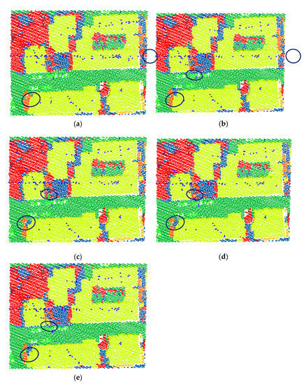
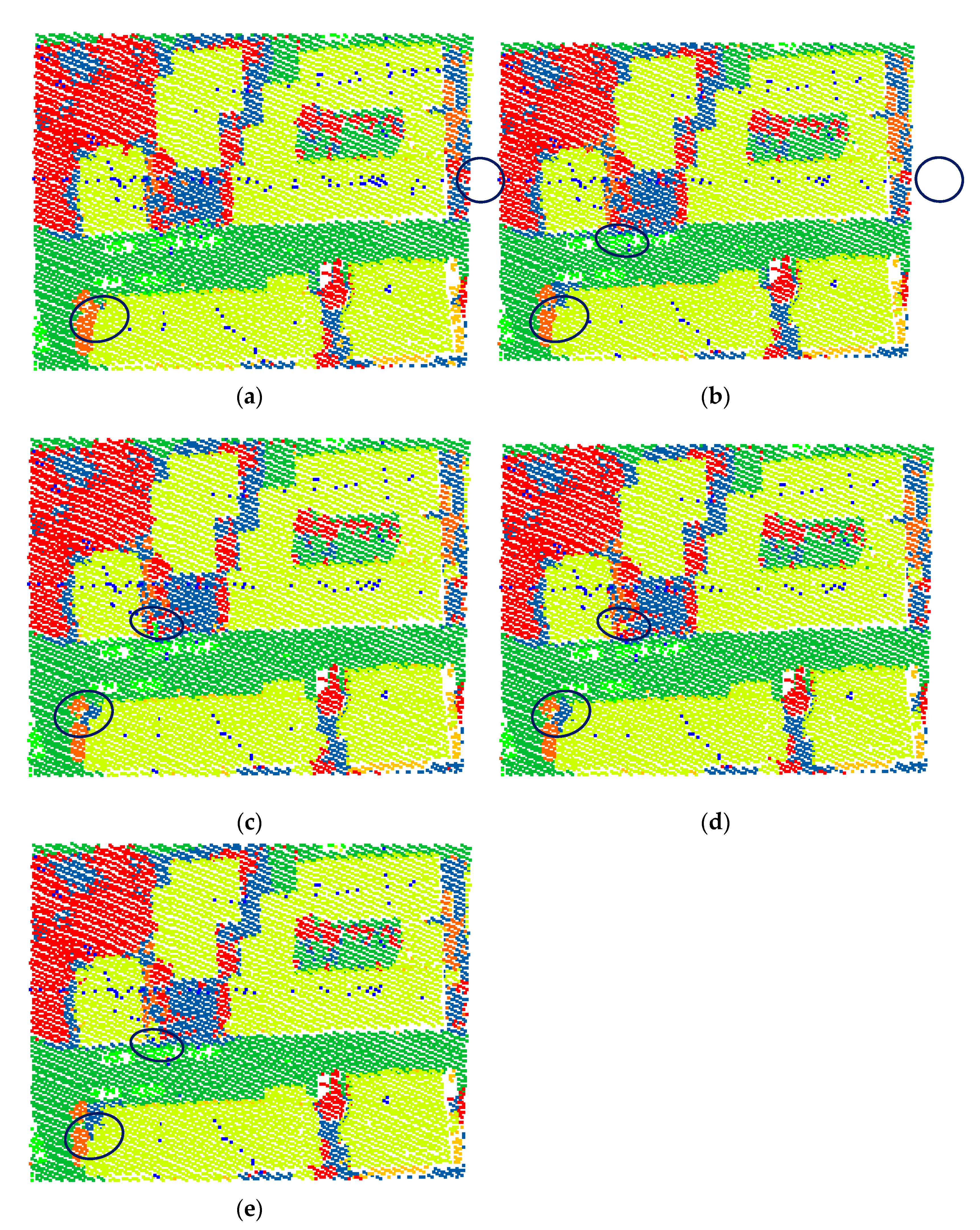
Figure 8. Classification results with different model configurations. (a) Baseline model, (b) baseline model with the proposed normal vector, (c) our model with both normal vector and atrous convolution, (d) our model with the normal vector, atrous convolution, and reweighted loss function, and (e) ground truth. The black circled parts highlight the differences among (a–e). (a) Baseline, (b) Ours (normal vector), (c) Ours (normal vector and atrous convolution), (d) Ours (final), (e) Ground truth.

To verify the effect of geometric input features on semantic segmentation, further comparative experiments were carried out. The network models of each experimental group were based on RandLA-Net. Only the local feature attention module of the network model was changed, and the point cloud normal vector was embedded in its spatial position coding. Select k values of 10, 20, 30, 40, and 50 were used to calculate different point cloud normal vectors. The five groups of data were used to conduct experiments to obtain the point cloud classification results. The experimental results are shown in Table 5. As seen from Table 5, when the K value is 30, the optimal overall accuracy (OA) and average F1 value are obtained, and 30 is the optimal K value determined by the algorithm in this paper.

Table 5. Comparison of the different K values in calculating the normal vector of the point cloud.

Method	OA	Average F1
K = 10	93.22	88.95
K = 20	96.16	93.04
K = 30	96.92	94.76
K = 40	95.88	91.93
K = 50	94.84	90.44

4.5.2. Effectiveness of Atrous Convolution

As shown in Table 4, based on the baseline network, the model that embeds the normal vector of the point cloud, atrous convolution improves the overall accuracy (OA) and average F1 value by 0.3% and 0.3%, respectively. A comparison of Figure 8b,c shows that our model corrects the misclassified ground points.

At the same time, the model embeds the normal vector of the point cloud. Atrous convolution is carried out in the contrast experiment with different dilation rates, with dilation rates of 2, 5, 8, and 11 used in the model. The classification performance is evaluated in terms of overall accuracy (OA) and average F1 value. Table 6 shows the classification results with different dilation ratios.

Table 6. Comparison of different dilation rates of atrous convolution.

Method	OA	Average F1
Rate = 2	0.954	0.939
Rate = 5	0.972	0.951
Rate = 8	0.960	0.930
Rate = 11	0.935	0.889

As shown in Table 6, when the dilation rate of atrous convolution is moderate (rate = 5), the model achieves the best classification performance because when the dilation rate is too small, the receptive field will be small, and greater neighborhood information involves more point cloud features. With the increase in the dilation rate, the point cloud increases the local receptive field, which helps to obtain more stable and fine-grained point cloud characteristics, thus improving the classification results. However, using a dilation rate that is too large will also decrease the classification performance. When the dilation rate = 5, our model performs best and presents an overall accuracy (OA) of 97.2% and an average F1 value of 95.1%.

4.5.3. Effectiveness of the Reweighted Loss Function

Table 4 shows that the reweighted method proposed in this paper is more suitable for point cloud classification with unbalanced categories. Compared with the original loss function, the improved loss function improves the overall accuracy (OA) and average F1 by 0.7% and 1.0%, respectively. A comparison of Figure 8 8c,d shows that our model corrects the misclassified building roof points.

To test the impact of different loss functions on the performance of point cloud classification, based on the baseline network and using the model of embedded point cloud normal vector and atrous convolution, this paper chose the cross-entropy loss function, weighted cross-entropy loss function, and reweighted loss function contrast experiment. The weighted cross-entropy loss function is weighted by the frequency of each type of point cloud, and the results are shown in Table 7.

Table 7. Comparison of the different loss function.

Method	OA	Average F1
Cross entropy	0.972	0.949
Weighted cross-entropy	0.972	0.951
Reweighted cross-entropy	0.979	0.961

As seen from Table 7, the reweighted cross-entropy loss function has an improved overall accuracy (OA) and average F1 value by 0.7% and 1.2%, respectively, compared with the cross-entropy loss function without weight. The reweighted loss function can solve the overfitting problem caused by the uneven distribution of the number of point clouds to a certain extent and can improve the accuracy of small target point clouds. The improved loss function proposed in this paper can effectively improve the performance of the model.

4.5.4. Comparison of Computational Load

To further study the computational load (measured by training time and GPU memory) of the proposed method, we list the results of DANCE-Net [47], GADH-Net [46], GACNN [48], 3DCNN [49], and our module in Table 8. Note that all results are collected in a semantic segmentation task on the Vaihingen urban 3D semantic dataset with 4096 points. It can be seen from Table 8 that GACNN [48] takes the longest time to process point clouds because of the cumbersome construction steps of graph attention convolution. The calculation overhead of DANCE-Net [47] and GADH-Net [46] is also very large. Our model is based on simple random sampling and an efficient local feature aggregator, which can infer the semantic labels of the point cloud in a short time.

Table 8. The computation time, GPU memory, OA, and GPU of different approaches.

Method	Training Time (Hours)	GPU Memory	OA	GPU
DANCE-Net	10	24 GB	0.839	Nvidia Tesla K80
GADH-Net	7	2 × 12 GB	0.850	2 × Nvidia Titan Xp
GACNN	10	12 GB	0.832	Nvidia Titan Xp
3DCNN	0.5	11 GB	0.806	Nvidia RTX 2080Ti
Ours	1.5	11 GB	0.979	Nvidia RTX 2080Ti

The results show that the memory consumption of our method is similar to that of 3DCNN [49]. Moreover, the training time of our module is slightly longer than 3DCNN [49], and the OA value has increased by 17.3%. Overall, our network achieves a good trade-off between model complexity and performance. These prove the effectiveness of our model, which does not consume too much memory or time, while the complexity of the model increases, and the segmentation accuracy is improved.

5. Conclusions

Because of the problems of the existing convolutional neural networks—which can directly learn the features of a point cloud, such as missing local features, multiple processing links, and large amounts of calculations—this paper proposes the integration of normal vector features into an atrous convolution residual network to classify LiDAR point clouds. Based on the RandLA-Net network, the atrous convolution and the point cloud normal vector are embedded in the network to realize the classification of the LiDAR point clouds. Specifically, we propose a fusion atrous convolution residual module that integrates atrous convolution into the residual block structure. It expands the receptive field and realizes multiscale point feature learning to extract more representative local features from the point clouds. The point cloud normal vector is implanted in the network structure to realize the extraction of the deep features of the point cloud. It can mine the hidden geometric correlations from the neighborhood to the greatest extent. An improved loss function is proposed to solve the unbalanced distribution of point cloud categories, so that the details of small objects will not be excessively lost in the process of depth feature extraction. The integration of normal vector features into the atrous convolution residual network proposed in this paper can capture valuable fine-grained information of point clouds, enhance the features of point cloud objects, and filter out useless features of the point cloud. Therefore, the segmentation ability of the model in complex scenes is improved. The proposed model can process input point clouds of any size and directly predict the semantic labels of all input points in an end-to-end manner. Because the algorithm in this study is based on the feature extraction of the coding part, it has good portability and can be easily embedded into the point cloud classification algorithm. To prove the advantages of the proposed model, a test was carried out on the Vaihingen urban 3D semantic dataset in Germany. The evaluation index was used to analyze the test result, and the OA value of the dataset reached 97.9% and the average F1 value reached 96.1%. This finding indicates that the algorithm has a better segmentation effect than RandLA-Net, even for small objects, such as power lines and cars, and has achieved extremely fine-grained classification results. Although point clouds with similar features will interfere with each other, the algorithm in this paper can avoid interference to a certain extent and achieve point cloud classification well. This robust performance is attributed to the integration of the FACR module, which also proves the strong generalization ability of the network for point cloud classification in a complex urban environment.

Although the classification evaluation proves the effectiveness of the proposed algorithm in point cloud classification, there is still space for improvement. Due to the problem of scanning height and angle, the point cloud obtained by airborne LiDAR is sparser than that obtained by a ground 3D laser scanner, which makes point cloud segmentation more difficult. The fusion of airborne LiDAR point clouds and aerial images can achieve a better segmentation effect. The experiment found that when there are too few points of some ground objects, the data processing will be limited, and the segmentation accuracy is insufficient. Improving the accuracy under the condition of a small number of point clouds will be an important direction for future point cloud classification research.

References

- Xu, Y.; Ye, Z.; Yao, W.; Huang, R.; Tong, X.; Hoegner, L.; Stilla, U. Classification of LiDAR point clouds using supervoxel-based detrended feature and perception-weighted graphical model. IEEE J. Sel. Top. Appl. Earth Obs. Remote Sens. 2019, 13, 72–88. [Google Scholar] [CrossRef]
- Wang, L.; Zhang, Y.; Wang, J. Map-based localization method for autonomous vehicles using 3D-LIDAR. IF AC-Pap. 2017, 50, 276–281. [Google Scholar]
- Hebel, M.; Arens, M.; Stilla, U. Change detection in urban areas by object-based analysis and on-the-fly comparison of multi-view ALS data. ISPRS J. Photogramm. Remote Sens. 2013, 86, 52–64. [Google Scholar] [CrossRef]
- Bassier, M.; Vergauwen, M. Topology reconstruction of BIM wall objects from point cloud data. Remote Sens. 2020, 12, 1800. [Google Scholar] [CrossRef]
- Polewski, P.; Yao, W.; Heurich, M.; Krzystek, P.; Stilla, U. Detection of fallen trees in ALS point clouds using a normalized cut approach trained by simulation. ISPRS J. Photogramm. Remote Sens. 2015, 105, 252–271. [Google Scholar] [CrossRef]
- Pan, Y.; Dong, Y.; Wang, D.; Chen, A.; Ye, Z. Three-dimensional reconstruction of structural surface model of heritage bridges using UA V-based photogrammetric point clouds. Remote Sens. 2019, 11, 1204. [Google Scholar] [CrossRef] [Green Version]
- Ene, L.T.; Erik, N.; Gobakken, T.; Bollandsås, O.; Mauya, E.; Zahabu, E. Large-scale estimation of change in aboveground biomass in miombo woodlands using airborne laser scanning and national forest inventory data. Remote Sens. Environ. 2017, 188, 106–117. [Google Scholar] [CrossRef]
- Jiang, H.; Yan, F.; Cai, J.; Zheng, J.; Xiao, J. End-to-end 3D point cloud instance segmentation without detection. In Proceedings of the IEEE/CVF Conference on Computer Vision and Pattern Recognition, Washington, DC, USA, 16–18 June 2020; pp. 12796–12805. [Google Scholar]
- Yang, B.S.; Liang, F.X.; Huang, R.G. Research progress, challenges and trends of 3D laser scanning point cloud data processing. J. Surv. Mapp. 2017, 46, 1509–1516. [Google Scholar]
- Lalonde, J.F.; Unnikrishnan, R.; Vandapel, N.; Hebert, M. Scale selection for classification of point-sampled 3D surfaces. In Proceedings of the Fifth International Conference on 3-D Digital Imaging and Modeling, Ottawa, ON, Canada, 16–18 June 2005; pp. 285–292. [Google Scholar]
- Gao, Z.H.; Liu, X.W. Support vector machine and object-oriented classification for urban impervious surface extraction from satellite imagery. In Proceedings of the IEEE 2014 Third International Conference on Agro-Geoinformatics, Beijing, China, 11–14 August 2014; IEEE: New York, NY, USA, 2014; pp. 1–5. [Google Scholar]
- Miao, X.; Heaton, J.S. A comparison of random forest and Adaboost tree in ecosystem classification in east Mojave Desert. In Proceedings of the IEEE 2010 18th International Conference on Geoinformatics, Beijing, China, 18–20 June 2010; IEEE: New York, NY, USA, 2010; pp. 1–6. [Google Scholar]
- Wang, C.S.; Shu, Q.Q.; Wang, X.Y.; Guo, B.; Liu, P.; Li, Q. A random forest classifier based on pixel comparison features for urban LiDAR data. ISPRS J. Photogramm. Remote Sens. 2019, 48, 75–86. [Google Scholar] [CrossRef]
- Schmidt, A.; Niemeyer, J.; Rottensteiner, F.; Soergel, U. Contextual classification of full waveform lidar data in the Wadden Sea. IEEE Geosci. Remote Sens. Lett. 2014, 11, 1614–1618. [Google Scholar] [CrossRef]
- Shapovalov, R.; Velizhev, A.; Barinova, O. Non-associative Markov networks for 3D point cloud classification. Int. Arch. Photogramm. Remote Sens. Spat. Inf. Sci. 2010, XXXVIII, 103–108. [Google Scholar]
- Zhu, Q.; Li, Y.; Hu, H.; Wu, B. Robust point cloud classification based on multi-level semantic relationships for urban scenes. ISPRS J. Photogramm. Remote Sens. 2017, 129, 86–102. [Google Scholar] [CrossRef]
- Hatt, M.; Parmar, C.; Qi, J.; Naqa, I. Machine (deep) learning methods for image processing and radiomics. IEEE Trans. Radiat. Plasma Med Sci. 2019, 3, 104–108. [Google Scholar] [CrossRef]
- Li, W.; Zhu, J.; Fu, L.; Zhu, Q.; Xie, Y.; Hu, Y. An augmented representation method of debris flow scenes to improve public perception. Int. J. Geogr. Inf. Sci. 2021, 35, 1521–1544. [Google Scholar] [CrossRef]
- Kong, W.; Dong, Z.Y.; Jia, Y.; Hill, D.; Xu, Y.; Zhang, Y. Short-term residential load forecasting based on LSTM recurrent neural network. IEEE Trans. Smart Grid 2017, 10, 841–851. [Google Scholar] [CrossRef]
- Sokkhey, P.; Okazaki, T. Development and optimization of deep belief networks applied for academic performance prediction with larger datasets. IE Trans. Smart Process. Comput. 2020, 9, 298–311. [Google Scholar] [CrossRef]
- Qi, C.R.; Su, H.; Mo, K.; Guibas, L. Pointnet: Deep learning on point sets for 3d classification and segmentation. In Proceedings of the IEEE Conference on Computer Vision and Pattern Recognition, Honolulu, HI, USA, 21–25 July 2017; IEEE: New York, NY, USA, 2017; pp. 652–660. [Google Scholar]
- Hu, Q.; Yang, B.; Xie, L.; Rosa, S.; Guo, Y.; Wang, Z.; Markham, A. RandLA-Net: Efficient semantic segmentation of large-scale point clouds. In Proceedings of the IEEE/CVF Conference on Computer Vision and Pattern Recognition, Seattle, WA, USA, 13–19 June 2020; pp. 11108–11117. [Google Scholar]
- Zuo, Z.; Zhang, Z.; Zhang, J. Urban LIDAR point cloud classification method based on regional echo ratio and topological recognition model. China Lasers 2012, 39, 195–200. [Google Scholar]
- Brodu, N.; Lague, D. 3D terrestrial lidar data classification of complex natural scenes using a multi-scale dimensionality criterion: Applications in geomorphology. ISPRS J. Photogramm. Remote Sens. 2012, 68, 121–134. [Google Scholar] [CrossRef] [Green Version]
- Becker, C.; Häni, N.; Rosinskaya, E.; d’Angelo, E.; Strecha, C. Classification of aerial photogrammetric 3D point clouds. ISPRS Ann. Photogramm. Remote Sens. Spat. Inf. Sci. 2017, 84, 287–295. [Google Scholar] [CrossRef] [Green Version]
- Guo, B.; Huang, X.; Zhang, F.; Wang, Y. Jointboost point cloud classification and feature dimension reduction considering spatial context. Acta Surv. Mapp. 2013, 42, 715–721. [Google Scholar]
- Niemeyer, J.; Rottensteiner, F.; Soergel, U. Contextual classification of lidar data and building object detection in urban areas. ISPRS J. Photogramm. Remote. Sens. 2014, 87, 152–165. [Google Scholar] [CrossRef]
- Niemeyer, J.; Rottensteiner, F.; Soergel, U.; Heipke, C. Hierarchical higher order crf for the classification of airbone lidar point clouds in urban areas. Int. Arch. Photogramm. Remote Sens. Spatial Inf. Sci. 2016, 41, 655–662. [Google Scholar] [CrossRef] [Green Version]
- Su, H.; Maji, S.; Kalogerakis, E.; Learned-Miller, E. Multi-view convolutional neural networks for 3D shape recognition. In Proceedings of the IEEE International Conference on Computer Vision, Santiago, Chile, 13–16 December 2015; pp. 945–953. [Google Scholar]
- Alonso, I.; Riazuelo, L.; Montesano, L.; Murillo, A. 3D-MiniNet: Learning a 2D representation from point clouds for fast and efficient 3D LIDAR semantic segmentation. IEEE Robot. Autom. Lett. 2020, 5, 5432–5439. [Google Scholar] [CrossRef]
- Maturana, D.; Scherer, S. Voxnet: A 3D convolutional neural network for real-time object recognition. In Proceedings of the 2015 IEEE/RSJ International Conference on Intelligent Robots and Systems (IROS), Hamburg, Germany, 28 September–3 October 2015; IEEE: New York, NY, USA, 2015; pp. 922–928. [Google Scholar]
- Meng, H.Y.; Gao, L.; Lai, Y.K.; Manocha, D. VV-Net: Voxel VAE net with group convolutions for point cloud segmentation. In Proceedings of the IEEE/CVF International Conference on Computer Vision, Seoul, Korea, 27 October–3 November 2019; IEEE: New York, NY, USA, 2019; pp. 8500–8508. [Google Scholar]
- Hegde, V.; Zadeh, R. FusionNet: 3D Object Classification Using Multiple Data Representations. arXiv 2016, arXiv:1607.05695. [Google Scholar]
- Qi, C.R.; Yi, L.; Su, H.; Guibas, L.J. Pointnet++: Deep hierarchical feature learning on point sets in a metric space. arXiv 2017, arXiv:1706.02413. [Google Scholar]
- Jiang, M.; Wu, Y.; Zhao, T.; Lu, C. PointSIFT: A SIFT-like network module for 3D point cloud semantic segmentation. arXiv 2018, arXiv:1807.00652. [Google Scholar]
- Zhao, H.; Jiang, L.; Fu, C.W.; Jia, J. PointWeb: Enhancing Local Neighborhood Features for Point Cloud Processing. In Proceedings of the IEEE/CVF Conference on Computer Vision and Pattern Recognition, Long Beach Convention & Entertainment Center, Los Angeles, CA, USA, 15–21 June 2019; IEEE: New York, NY, USA, 2019; pp. 5565–5573. [Google Scholar]
- Wang, C.; Samari, B.; Siddiqi, K. Local spectral graph convolution for point set feature learning. In Proceedings of the European Conference on Computer Vision (ECCV), Munich, Germany, 8–14 September 2018; pp. 52–66. [Google Scholar]
- Landrieu, L.; Simonovsky, M. Large-scale point cloud semantic segmentation with super point graphs. In Proceedings of the IEEE Conference on Computer Vision and Pattern Recognition, Salt Lake City, UT, USA, 18–22 June 2018; pp. 4558–4567. [Google Scholar]
- Li, Y.Y.; Bu, R.; Sun, M.; Wu, W.; Di, X.; Chen, B. PointCNN: Convolution on χ-transformed points. Adv. Neural Inf. Process. Syst. 2018, 31, 820–830. [Google Scholar]
- Xu, Y.F.; Fan, T.Q.; Xu, M.Y.; Zeng, L.; Qiao, Y. SpiderCNN: Deep learning on point sets with parameterized convolutional filters. In Proceedings of the European Conference on Computer Vision (ECCV), Munich, Germany, 8–14 September 2018; pp. 87–102. [Google Scholar]
- He, K.; Zhang, X.; Ren, S.; Sun, J. Deep residual learning for image recognition. In Proceedings of the IEEE Conference on Computer Vision and Pattern Recognition (CVPR), Las Vegas, NV, USA, 26 June–1 July 2016; IEEE: New York, NY, USA, 2016; pp. 770–778. [Google Scholar]
- Yu, F.; Koltun, V. Multi-scale context aggregation by dilated convolutions. In Proceedings of the International Conference on Learning Representations (ICLR), Caribe Hilton, San Juan, Puerto Rico, 2–4 May 2016; IEEE: New York, NY, USA; pp. 1–13. [Google Scholar]
- Cui, Y.; Jia, M.; Lin, T.Y.; Song, Y.; Belongie, S. Class-balanced loss based on effective number of samples. In Proceedings of the IEEE/CVF Conference on Computer Vision and Pattern Recognition (CVPR), Long Beach, CA, USA, 15–21 June 2019; pp. 9260–9269. [Google Scholar]
- Wen, C.; Yang, L.; Li, X.; Peng, L.; Chi, T. Directionally constrained fully convolutional neural network for airborne LiDAR point cloud classification. ISPRS J. Photogramm. Remote Sens. 2020, 162, 50–62. [Google Scholar] [CrossRef] [Green Version]
- Thomas, H.; Qi, C.R.; Deschaud, J.E.; Marcotegui, B.; Goulette, F.; Guibas, L.J. KPConv: Flexible and deformable convolution for point clouds. In Proceedings of the IEEE/CVF International Conference on Computer Vision (ICCV), Seoul, Korea, 27 October–3 November 2019; IEEE: New York, NY, USA, 2020; pp. 6411–6420. [Google Scholar]
- Li, W.; Wang, F.D.; Xia, G.S. A geometry-attentional network for ALS point cloud classification. ISPRS J. Photogramm. Remote Sens. 2020, 164, 26–40. [Google Scholar] [CrossRef]
- Li, X.; Wang, L.; Wang, M.; Wen, C.; Fang, Y. DANCE-NET: Density-aware convolution networks with context encoding for airborne LiDAR point cloud classification. ISPRS J. Photogramm. Remote Sens. 2020, 166, 128–139. [Google Scholar] [CrossRef]
- Wen, C.; Li, X.; Yao, X.; Peng, L.; Chi, T. Airborne LiDAR point cloud classification with global-local graph attention convolution neural network. ISPRS J. Photogramm. Remote Sens. 2021, 173, 181–194. [Google Scholar] [CrossRef]
- Özdemir, E.; Remondino, F.; Golkar, A. An efficient and general framework for aerial point cloud classification in urban scenarios. Remote Sens. 2021, 13, 1985. [Google Scholar] [CrossRef]
Publisher’s Note: MDPI stays neutral with regard to jurisdictional claims in published maps and institutional affiliations. |
© 2021 by the authors. Licensee MDPI, Basel, Switzerland. This article is an open access article distributed under the terms and conditions of the Creative Commons Attribution (CC BY) license (https://creativecommons.org/licenses/by/4.0/).