Abstract
A multi-temporal satellite radar interferometry technique is used for deriving the actual surface displacement patterns in a slope environment in Romania, in order to validate and improve a landslide susceptibility map. The probability the occurrence of future events is established using a deterministic approach based on a classical one-dimension infinite slope stability model. The most important geotechnical parameters for slope failure in the proposed study area are cohesion, unit weight and friction angle, and the triggering factor is a rapid rise in groundwater table under wetting conditions. Employing a susceptibility analysis using the physically based model under completely saturated conditions proved to be the most suitable scenario for identifying unstable areas. The kinematic characteristics are assessed by the Small BAseline Subsets (SBAS) interferometry technique applied to C-band synthetic aperture radar (SAR) Sentinel-1 imagery. The analysis was carried out mainly for inhabited areas which present a better backscatter return. The validation revealed that more than 22% of the active landslides identified by InSAR were predicted as unstable areas by the infinite slope model. We propose a refinement of the susceptibility map using the InSAR results for unravelling the danger of the worst-case scenario.
1. Introduction
Landslides are among the most significant natural events that cause human and material losses worldwide. Conventionally, landslides are defined as the movement of a rock or soil mass along a slope [1]. In Romania, landslides are the most frequently occurring slope processes in the Cretaceous and Paleogene flysch sector of the Eastern Carpathians, and in the Subcarpathian region of Neogene molasse deposits e.g., [2,3,4,5,6]. The Carpathian and Subcarpathian Bend area (the Curvature Carpathians) is especially susceptible to landslides, amid intense local seismic activity coupled with neotectonics, both of which favor instability e.g., [7,8]. Furthermore, pluviometric regime specificities, i.e., alternating wet and dry cycles, play a role in setting off shallow planar and translational slides [6,7,9]. According to Surdeanu [9], over the past 130 years, four pluviometric excess periods (1912–1913; 1939–1942; 1970–1972 and 2004–2005) induced most of slope failures in Romania’s flysch and molasse areas. Most rainfall-triggered landslides are shallow and directly linked to subsurface hydrological processes. Given the broad countrywide extent of the phenomena, in the 1980s, Romania joined the global cluster of countries where critical prediction studies are conducted on shallow rainfall-induced landslides. Most predictions of rainfall-induced landslides are presently based on landslide susceptibility maps and on the correlation between landslide occurrence and rainfall thresholds [10,11]. Landslide susceptibility maps, validated by direct field observations, are crucial elements of prevention studies and risk management applications for landslide-prone areas.
Landslide susceptibility is the spatial (geographical) likelihood of landslide occurrence, given a set of local conditioning factors, regardless of the sliding recurrence period e.g., [12,13,14]. For the present study, we propose comparing and fusing both traditional and modern techniques with the objective to revise and enhance a landslide susceptibility map of the hilly belt along Prahova Valley, which is among the most densely built sectors of Romania’s Curvature region [8] (Figure 1). Prahova Valley is also a major communication route between the capital and Transylvania, where an important motorway is planned to be built.
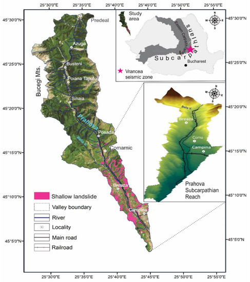
Figure 1.
Study area and shallow landslide distribution. Base map: Landsat 8 scenes from 20 August 2019, downloaded from Earth Resources Observation and Science (EROS) Center, USGS. DEM obtained from 1:25,000 topographic maps.
The traditional technique we employ is the one-dimension infinite slope stability model, the oldest and most physically (geotechnically) simple model, based on the limit equilibrium theory, which is used to ascertain a given slope’s safety factor [11,14,15,16,17,18,19,20,21]. The safety factor (SF) is computed as the dimensionless ratio between the main forces that act on a slope: shear stress, which provokes motion along a potential failure surface, and shear strength (described by the Mohr–Coulomb approach). In the assessment of the infinite slope model, it is assumed that the slip plane and water table are parallel to the slope’s topographic surface [21,22].
The infinite slope model is suitable for shallow sliding with planar failure surfaces, where the sliding depth is considerably lower than the slope’s length [23]. Shallow landslides are common translational slips and are characterized by a thin soil cover (usually no more than a few meters [24]). These slope movements dominate landslide processes in hilly areas, as evinced by numerous specialized studies e.g., [25]. The Carpathian and Subcarpathian Prahova Valley, the proposed study area, is a mountainous and hillslope environment that is highly fitting for testing the infinite slope model’s robustness, as well as for determining its limitations (Figure 1).
In order to enhance the assessment of landslide susceptibility maps across extensive areas, the infinite slope model can be integrated in Geographic Information System environments (GIS), as this is a pixel-based calculation that considers each raster cell separately e.g., [26,27,28,29,30,31,32,33,34,35]. However, a variable degree of uncertainty is linked to the complex and inherent variability of geological features when applying physical models over large areas. The validation process is thus a necessary phase of determining the extent to which the result reflects an accurate image of the real settings according to available field data. The present study tests the landslide susceptibility map against field survey landslide inventory database entries alongside interferometric synthetic aperture radar (InSAR) deformation maps, in a statistically oriented manner.
InSAR is a satellite monitoring method that enables the first-ever capability to effortlessly derive surface displacement over extensive areas at a low cost [36]. The main condition for detection is for the displacement to affect radar coherent targets, such as man-made features, open rocks or land [37,38]. An additional noteworthy benefit of this technique consists of enabling users to derive displacement rates of high vertical accuracy (sub-millimeter) [39], with a relatively high temporal resolution of up to 6 days in case of Sentinel-1 A/B satellites above Europe and global availability of free satellite data [40]. InSAR monitoring is also able to deliver a different outlook over a given study area, either by identifying new, undiscovered developing landslides, or by validating others that had been identified previously [37]. What sets InSAR deformation maps apart from susceptibility maps generated using conventional methods is the kinematic characterization of landslides, which is useful for validating and bringing pre-existing landslide inventories up to date. In addition, dynamic characteristics can be used as an input for mechanical models describing the dynamics of landslide processes.
In the last two decades, several multi-temporal interferometric methods have been successfully applied for updating and validating landslide inventories by combining traditional geomorphological information with observations of ground displacement analysis, from which the most recurring were the Persistent Scatterers interferometry [41,42,43,44,45,46] and the Small BAseline Subset interferometry [47,48,49,50,51,52]. Due to its enhanced capabilities, the InSAR multi-temporal technique has been used in a multitude of studies for landslide detection. Several satellite data are normally used for landslides studies as the satellite imagery acquired in C-band, such as historical satellites ERS and Envisat [46,52,53,54,55], or the more recent data from satellites Radarsat and Sentinel-1 [45,56,57,58], X-band satellites—TerraSAR-X [44,59] and L-band satellites—ALOS PALSAR [48,54]. These studies use satellite interferometry as the main tool for assessing slope instability, and usually compare these data with geodetic measurements, field recognition or optical imagery for validation. Righini et al. [46] use deformation maps obtained with satellite interferometry to update a pre-existing landslide inventory in Biferno Basin, Italy. Bardi et al. [59] use InSAR techniques to detect slope instability and combine the InSAR results with independent statistical analysis and activity models to characterize the activity state of the earth surface in specific regions.
In Romania, the use of satellite interferometry for studying landslides is recent; currently the only study is by Necula [60], which focuses on the detection of active landslides in a habited area from Iași county using multi-temporal techniques applied for Sentinel-1 imagery.
In this study, we propose applying the SBAS interferometric technique for detecting slope instability. Additionally, this technique is also used as a complementary tool to quantify its performance in terms of predicting landslide-prone areas compared to the infinite slope model. We propose a comparison between the susceptibility maps derived using the classical one-dimension infinite slope stability model and the InSAR deformation map. Because of InSAR characteristics, the study area focuses on inhabited communities which present coherent radar targets. As data sources, we selected the C-band Sentinel-1A and B European Space Agency (ESA) satellites. These satellites were considered suitable for the current study due to their free availability and data continuity since 2014, as well as their enhanced temporal resolution. For data processing we use the Berardino [47] SBAS algorithm due to its ability to enhance coherence, reduced noise of interferograms, and to identify nonlinear movements.
2. Tectonic and Geological Settings of the Study Area
The study area consists of the Carpathian and Subcarpathian Prahova Valley, which separates the Eastern and Southern Carpathians over 56 km (Figure 1). The Prahova Valley is among the most densely populated sectors of Romania’s Carpathian and Subcarpathian region, as well as being the location of an important trans-Carpathian roadway connecting Balkan countries and Western Europe [8,35]. Over the past century, a wide range of infrastructure projects have been implemented along the Prahova Valley, including roads, railways, bridges, watercourse regulation and bank protection measures, as well as oil and in-channel gravel extraction activities, all of which changed the local natural environment to varying degrees [61].
The Carpathian stretch of Prahova river consists of a series of narrow reaches spaced out by minor tectonic-erosive depressions. The mountain valley slopes feature four fluvial terraces. Diluvial slope formations primarily consist of sandstone fragments and limestone, cemented by a clay-silt matrix (the flysch facies) that determines slope instability notably in areas with no abundant alpine vegetation. A 2 m diluvium layer prevails, below which a highly fractured and altered flysch facies is present, down to a depth of approximately 5 m. Flysch deposits are folded in serried synclines and anticlines. Deep-seated landslides and rock falls spread on the hanging wall of reverse faults. Most of these slides are of Pleistocene age, stabilized under forested conditions [9,62,63,64,65].
One of the defining elements of the present study area is the large Subcarpathian erosive basin spread between the Comarnic–Breaza and Câmpina settlements in which Prahova river carved four terraces [8,14]. The erosional river valley is lowered in the northern part, in the Barremian–Aptian flysch zone. This northern part is represented by a marl-calcareous flysch with thin micro-breccia layers, known as the Comarnic formation, flanked on its southern edge by the Senonian red marls (Gura Beliei formation) and a Paleogene marl-sandstone flysch formation (the Sotrile flysch). Downstream, the confluence of the Belia and Prahova rivers outcrops the post-tectonic bedcover [8,63]. From the locality of Breaza to Cornu, the Breaza syncline extends in a west-to-east direction (Figure 1), has developed symmetrical flanks and is axially faulted. The structure’s southern sector is elevated along the Breaza fault [8,14], where is represented by lower-Miocene deposits, such as the Cornu strata and the Brebu conglomerates. In the southern part of the Cornu locality, the molassic deposits are present with the Miocene–Pliocene–Lower Pleistocene strata, and they form the Miocene–Pleistocene zone (Figure 2).
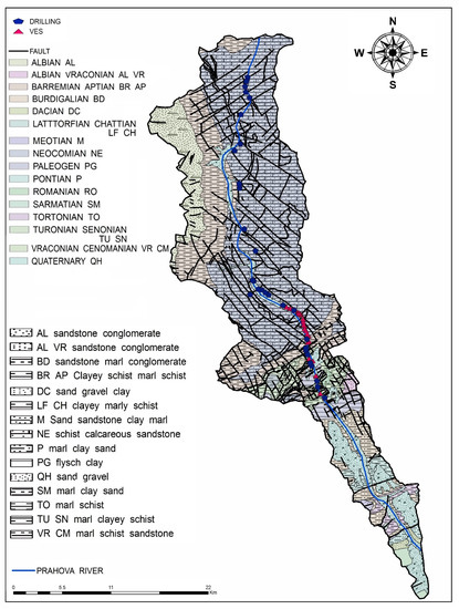
Figure 2.
Geological and lithological settings. We used the color codes in the geological map.
In general, shallow-to-medium deep landslides are quite frequent in the Subcarpathian area. The active processes, affecting over 60% of scarp surfaces, are triggered by intense or prolonged rainfall periods [8,14]. Rainfall-induced landslide reactivation also affects bodies and scarps of older landslides, and the slopes where the land is used for intensive grazing. In this study, we use a detailed landslide inventory of over 400 landslides (Figure 1) for model evaluation along with geologic and morphologic information. The landslide inventory resulted from repeated research campaigns carried out by Prof. Armaș in the study area over a 5 years period. A detailed description of the environmental conditions, landslide types, forcings (precipitation, groundwater, earthquakes, river erosion, human impact), motion and evolution pattern can be found in previous work of the author [8,61,66,67,68]. From the landslide database, only shallow, slow-moving slides are selected for this study.
3. Data and Modelling Parameters
3.1. Spatial Database and Input Parameters
The deterministic approach necessitates a high volume of data, e.g., a high-resolution digital elevation model (DEM) and geomorphological specificities (slope angles, sine and cosine), existing thematic maps, a series of detailed field surveys, geomorphological investigations and mapping procedures, and numerous laboratory tests. Our DEM is obtained by the automatic interpolation of 5 and 10 m contour lines derived from existing 1:25,000 and 1:5000 topographic maps, enhanced with data from a 1 m resolution digital elevation model achieved by airborne LiDAR, specifically performed in 2012 along the valley bottom [35]. The geotechnical input parameters such as cohesion and friction angle of slope materials are obtained from laboratory analysis. The data we use are part of a larger 2014 geotechnical study for the Comarnic–Brasov motorway, and consists of geotechnical drillings, vertical electrical surveys (VES), geological mapping and geotechnical laboratory analysis, together with a detailed geological mapping completed in the autumn of 2017. In the 2014 geotechnical study, drilling was performed with wireline systems, with freshwater fluid and bio-degradable additives. The drilling diameter is 146 mm with a 100 mm core diameter, and both disturbed and undisturbed samples were collected. In the case of disturbed samples, they are collected directly from the core box. The undisturbed samples ore obtained with Shelby tube from the drilling hole. The undisturbed samples are 87 mm in diameter and are 500 mm long. The following laboratory tests are performed by a private company in a grade I (ISO9001 9001) geotechnical laboratory:
- Granulometry analysis;
- Natural moisture analysis (w);
- Plasticity analysis—Atterberg limits (liquid limit WL, plastic limit WP, consistency index IC, plasticity index IP);
- Structure index analysis (moist volumetric weight γ, dry volumetric weight γd, voids index e, porosity n);
- Monoaxial compression resistance (compression resistance Rc).
Although these laboratory parameters might represent point singularities and unique characteristics, they can be extrapolated as a general description of each lithological unit identified in the study area (Table 1).

Table 1.
Litho-stratigraphic classes and geotechnical parameters used in the study area.
Another important set of data are obtained from a detailed vertical electrical sounding (VES) performed by a private company (Search Corporation SRL, Bucharest, Romania—http://www.searchltd.ro/, accessed on 1 May 2021). VES provide the electrical resistivity (conductivity) of rocks using the flow of an induced electric current inside the earth. VES is performed at 46 stations along the Prahova Valley, and provides valuable information regarding the resistivity distribution, which can be interpreted in terms of depth-location and thickness of several main geological layers (Figure 2). Therefore, we obtain a detailed spatial image of various subsurface lithologic units, and also estimate the depths of bedrock surfaces.
Our geological mapping is performed using data from walk-over surveys, geological site investigations in outcrops and anthropic openings and cuttings, excavations, and several existing water wells. Finally, we merge all the results with those from 1/200,000 and 1/50,000 geological maps and propose the stratigraphic succession shown in Figure 2 and Table 1.
Field-mapping, with stereoscopic interpretation of aerial photographs, reveals the location of unhooks and normal and reverse faults. We obtain a detailed complex tectonic pattern consisting of 29 well identified unhooks, 342 normal faults and 144 reverse faults (Figure 2).
3.2. InSAR Data
The Prahova study area is covered by Sentinel-1 images acquired in two frames, on descending and ascending orbits (Table 2). In the study area, slow-developing landslides are expected, therefore stacks of images with a temporal resolution of 1 month were considered in order to reduce the computing time. Two stacks of 123 images acquired between October 2014 and October 2018, out of which are 62 on ascending orbit and 61 are on descending orbit, were processed separately in order to derive surface motion from different geometries.
Table 2.
Sentinel-1B images parameters.
Figure 3 presents the extent of the area covered by the images acquired on each orbit. The temporal resolution of the Sentinel-1A satellites was initially of 12 days, but increased later to 6 days after the launch of Sentinel-1B satellite.
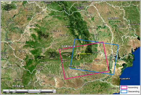
Figure 3.
The extent of the areas including Prahova Valley that are covered by the acquisition orbit of the Sentinel-1A and Sentinel-1B satellites. Map created in Esri. ArcGIS® and ArcMap™ 10.4.
The extent of the area selected for InSAR processing is conditioned by the limitations of the remote sensing technique and by the results obtained from the deterministic approach. Thus, the Carpathian area of the Prahova Valley is eliminated mainly due to a lack of coherent targets for the radar signal. In addition, a large difference between the Doppler centroids of the SAR images acquired in ascending orbit limit the common coverage area by all the images in the stack to the Subcarpathian reach of the valley.
4. Slope Stability Assessment Methods
4.1. The Infinite Slope Model
In order to compute the safety factor (SF) of slopes and to derive the landslide susceptibility map for a selected study area susceptible to translational landslides, a one-dimensional deterministic stability model (infinite slope model) is applied in a raster-based GIS environment (ILWIS) [22]. Figure 4 presents an outlook on the way in which slope specific stability is approached. The workflow is separated into three phases: the preparation (preliminary) phase, the analytical phase and the validation.
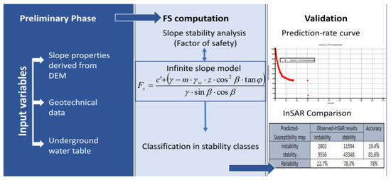
Figure 4.
General workflow.
The infinite slope model is seated on the limit-equilibrium approach and on the principle that failure occurs when disturbing forces exceed the capacity to resist of the earth materials [69]. The process is enhanced by the effects of water. A detailed description of the geotechnical, hydraulic, and geometric principles for the SF calculation is provided by Mergili et al. [70]. In this study, we calculate the SF using the same expression in Equation (1) as in [35], written in effective stresses without pore water pressure [22,71]:
where: c’ = effective cohesion (Pa = N/m2), γ = unit weight of soil (N/m3), z = depth of failure surface, m = the ratio of the groundwater level to the soil depth (dimensionless), γw = unit weight of water (N/m3), β = slope gradient (°) and ϕ = effective angle of shearing resistance (°).
Every parameter (except “m”) in Equation (1) represents a space variable, and we infer the SF for each pixel. The saturation depth “m” is the only time-dependent variable of the FS equation [35]. This ratio ranges from 0 to 1; 1 when the soil is completely water saturated, and 0 when the soil is dry. In the present study, we solely tested the worst-case scenario of fully saturated soil, as partial saturation is more challenging to approach geotechnically.
Despite the fact the study area is within the Vrancea seismic region, which is Europe’s most seismically active zone [72,73], in our model no external forces, such as seismic loading, are taken into account. Our approximation is valid because active, shallow landslides along the Prahova Valley are rainfall-triggered events, as identified in previous studies [3,7,8,35,66,67,68].
The landslide susceptibility maps are classified into three stability classes. For SF less than 1, the slope is in an unstable condition, and when SF is over 1.5, the slope is in a stable condition. For intermediate values of 1 or less then 1.5, the slope is considered to be in a meta-stable condition, and minor undermining factors can easily lead to instability [35].
4.2. InSAR Based Method
The SBAS technique [47] consists of an approach that reduces temporal and spatial decorrelation by deriving small baseline interferograms. Instead of using discrete coherent targets such as in the case of classic PS methods [41,42], SBAS exploits coherence over larger areas using Delaunay triangulation [74]. Because SBAS exploits coherent areas instead of discrete coherent targets, the technique is more useful for rural and natural areas.
The SBAS algorithm is applied using the SARscape software, provided by SARMAP. The steps of applying the SBAS algorithm involve pairing images for the generation of interferograms, and deriving residual height using the NASA Shuttle Radar Topographic Mission (SRTM) DEM with 1 Arc-Second Global, displacement velocity and displacement time series after the removal of atmospheric effects. Paired images are called masters and slaves. During the interferometric process, the images are co-registered in the geometry of the masters, taking into account temporal and spatial baseline-imposed restrictions. For the ascending stack, from a number of 62 images, we generate 807 interferograms that respect the constraints of a maximum temporal baseline of 365 days and a spatial baseline of 1200 m. After imposing the same constraints on the 61 images from the descending stacks, a number of 865 interferograms are also obtained. In the next step, the interferograms are filtered in order to remove the atmospheric, topographic and orbital influences on the phase variations. After that, each interferogram is inspected manually. A number of 3 low quality images from the ascending stack and 1 image from the descending stack and their corresponding interferograms are removed from the processing chain because of being affected by too large atmospheric artefacts and orbit errors that could not be corrected.
The final displacement time series for different coherent targets in the study area are obtained after applying a second atmospheric filtering for generating the final and cleaned displacement time series.
5. Modelling Results
5.1. Deterministic Approach
In this study, the one-dimension infinite slope stability model is employed to assess a shallow landslide susceptibility map across a mountainous and hilly region of Romania. For determining the safety level for valley slopes, an overall factor of safety of 1.0 is applied as a criterion for stability. Using slope angles, individual maps for the sine, cosine and the square of the cosine are calculated. Geotechnical data of slope materials are obtained from geological surveys, VES, boreholes, laboratory tests, and also from the literature. In our slope stability model, we use a series of thematic maps computed specifically for slope materials: soil thickness, cohesion, unit weight, and friction angle, and the slope failure susceptibility map using the deterministic approach under completely saturated conditions (Figure 5).
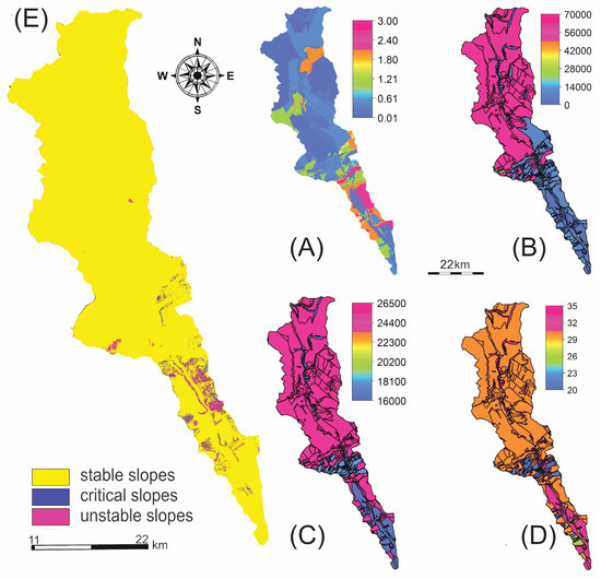
Figure 5.
The distributions of (A) soil thickness, m; (B) cohesion, N/m2; (C) unit weight, N/m3; (D) friction angle (˚). (E) Slope failure susceptibility map using the deterministic approach under completely saturated conditions.
Soil thickness refers to the thickness of the overburden and is computed from the depth to bedrock (Figure 5a). We consider the depth of the contact between the overburden and the bedrock as the slip plane of failure along a slope. The contact is established according to several data sources such as drillings, VES and specific literature e.g., [8,35,66,67,68]. Another source of data we use is the landslide inventory in which depths of the slip plane are reported. In the Subcarpathians, depths of the slip plane are between of −1 and −4 m, and in the Carpathians, a shallow depth of contact is measured, between −0.1 and −1 m. The difference is due to the geological particularities of the two areas. Hills are in general characterized by soft rocks with alternations of permeable and impermeable layers, while mountain slopes are covered by thick periglaciar debris and diluvial soil. Therefore, in the hilly area, there is a higher variation in the depth of the contact. In the mountains, the minimum soil depth is located on the Bucegi Mountains’ steep slope towards the Prahova river.
If we compare the Carpathian and the Subcarpathian areas in terms of geotechnical indices that directly influence landslides, we observe that in the Carpathians, where hard rocks (schist, sandstone, hard marls and conglomerates) are visible, the cohesion and the unit weight values are high, but the friction angles values are low. Hence, this area is prone only to rock sliding. On the other hand, in the Subcarpathians, characterized primarily by predominantly soft rocks (clays, marls, weathered conglomerate and sandstone, sands and silts), the cohesion and the unit weight values are lower, and the friction angle values are higher, favoring rainfall-induced landslides. When soil depths increase, slope angle, internal friction angle and wetting conditions gain importance [35,75,76]. We find that soil cohesion is more variable than the friction angle, as reported in previous studies [77].
Figure 5e displays the results of the landslide susceptibility under completely saturated conditions. The spatial distribution map reveals that this method is relevant only for hilly regions in our study area, which have more homogenous lithology, alternating permeable/impermeable soft rocks and larger deforested areas [8]. The Prahova river has a N–S oriented course along an important fault that cuts transversal the Miocene–Pliocene anticline and syncline system [35] (Figure 2). The slopes of the upper terraces are transformed into an erosion glacis, continued with a large colluvial–proluvial glacis that is developed on the terrace II tread. Terrace II is the largest and best-preserved fluvial terrace in the Subcarpathian sector. The slopes of terrace II are affected by active landslides that heavily erode the lowest terrace tread, which appears to act as a set of stability shoulders between the sliding areas [8]. This geomorphological pattern is well represented on the landslide susceptibility map, which classifies these slopes as unstable or in a critical state. In this study, we show that this pattern is confirmed also by the InSAR results.
5.2. InSAR Results
After processing the datasets acquired from ascending and descending orbits for the Prahova Valley, two deformation maps are achieved. An average number of 430,000 scatterers are obtained from each of the datasets within an area of 120 km2 and a spatial density of 850 point/km2. The realized maps show an average velocity of –0.5 mm/yr with a standard deviation of ± 0.4 mm/yr in the satellite’s line of sight. According to the literature, the stability threshold depends on the radar sensor used and the standard deviation of the PS dataset obtained, which is around ± 0.5 mm/yr. The most commonly defined value interval defined as stable for Sentinel-1-derived deformation maps is either between ± 1.5 mm/yr or ± 2 mm/yr [59,78]. In Figure 6, stable areas with a low movement amplitude (± 2 mm/yr) corresponding to stability are depicted in green, while areas affected by instability are emphasized in red if the target moved away from the sensor and blue if the target moves towards it. Both deformation maps show consistent movement patterns for areas with coherence values of at least 0.70, which indicates the high reliability of the results [42,47]. Some small artefacts can be observed in the deformation maps for the ascending and descending orbits (Figure 6), with differences occurring in the type of pattern shown at the same location (either movement away or towards the sensor). There are unstable areas that are clearly depicted in both deformation maps and areas with a limited degree of correspondence from one map to another. The hilly area in the north of the valley shows an inversion of the positive and negative movement patterns of points found at the same location in both maps.
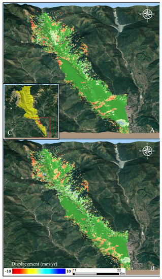
Figure 6.
Deformation maps over the Subcarpathian area derived from Sentinel-1 data acquired on (A) ascending orbit and (B) descending orbit. Red dots show movement of the target away from the sensor, blue dots show movement towards the sensor and green points stable areas. (C) locates the Subcarpathian study area. Map created in QGIS3 software. Base map: Landsat 8 scene from 20 August 2019, downloaded from Earth Resources Observation and Science (EROS) Center, USGS.
This is caused by the dependency between the satellite’s line of sight geometry in relation to the terrain slope, which influences the direction of the displacement depicted by the satellite. From a descending orbit, the sensor perceives the targets on the left slope as approaching it, while the targets on the right slope are distancing from the sensor. The influence of the satellite’s view geometry on movement patterns derived for hilly surfaces have been discussed also by other authors in the past, who recommended using both orbits and decomposing the results for a better depiction of the actual direction of the observed displacement [50]. However, the fact that negative and positive movement trends are found at the same location in both deformation maps is an indication that these areas show consistent movement patterns.
Because deformation maps (Figure 6) appear initially to exhibit sub-vertical displacements instead of translational movement as would be expected in the case of shallow landslides, the resulted displacement vectors obtained from ascending and descending orbits are decomposed on horizontal and vertical directions using points located in corresponding areas of 100 m2 from both images and the known viewing angle for each location (Figure 7A,B). From the representations of horizontal versus vertical linear velocities, we conclude that the predominant displacement in the study area is horizontal, surpassing the vertical velocity in areas affected by instability. In this case, the horizontal movement can be associated with a displacement down the slope, implying the existence of a translational displacement, characteristic to shallow landslides.
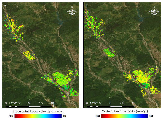
Figure 7.
Decomposition of vertical velocity values on horizontal (A) and vertical axes (B) for three areas of the Subcarpathian Prahova Valley (velocity units in mm/yr). In Figure 7A, negative values depict movement towards the west, while positive values show movement towards the east. In Figure 7B, negative values correspond to vertical subsidence while positive values represent vertical uplift.
6. Validation Procedure
6.1. The Prediction-Rate Curve
To confirm the validity of results, we use the prediction-rate curve [79]. The prediction-rate curve involves computing the conformity between the landslide susceptibility results and the empirical observed shallow landslides, as the inventoried landslide distribution in each susceptibility class [79,80,81].
The multi-temporal landslide inventory map we employ to validate the deterministic approach is obtained from a combination of field surveys and aerial imagery. For model evaluation, we focus on shallow active and latent landslides, considering an inventory of over 400 sites (Figure 1). In our validation approach, due to the mobility of shallow landslides especially during rainy periods, we use the entire landslide affected area.
The prediction-rate curve results are shown in Figure 8, using cumulative statistics.
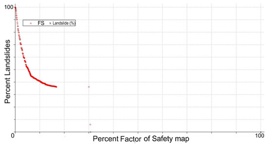
Figure 8.
The prediction-rate curve representing the cumulative percentage of triggered landslide correctly classified in each stability class on the y-axis (true positive rate), and the percentage of area classified as positive (i.e., unstable and critical units classified as positive) on the x-axis, ranked from most (SF < 1) to least susceptible (SF > 1).
The prediction-rate curve shows that almost all landslides along the Subcarpathian terrace slopes are located within the most hazardous 18% area of the susceptibility map, where the InSAR processing was also employed.
The comparison of mapped landslides and modelling results reclassified into two different classes (unstable/stable) is presented in a contingency table (Table 3). True positive refers to landslides located in areas classified as unstable and critical, and false positives outline areas predicted as susceptible but without landslides. True negative is when areas predicted as safe have no landslides, and false negative delineate the case when landslides occur in areas predicted as safe. Several quality measures are provided by linking together correct and incorrect classified positives (i.e., unstable areas) and negatives (i.e., stable areas) (Table 3).
Table 3.
Prediction errors (% of correctly and incorrectly predicted pixels) and accuracy statistics.
Although the deterministic model is data demanding and requires a high degree of simplification of input values, the accuracy statistics derived from the contingency matrix show that the model is able to correctly classify especially safety areas (93% being correctly classified) and non-observations of the sliding phenomenon (0.3%). The result can be also related to the fact that the susceptibility map is a prediction for the hazard of future landslides and not the hazard itself.
Considering the area in Figure 7 as stable should be subjected to future scrutiny, as there might be errors generated by the limitations of the method we used. The large apparent stable area in the reach of the Prahova Valley is the result of old deep-seated landslides, downfalls and debris, reinforced by vegetation, providing a non-realistic slope stability. The future motorway plans along the Prahova river corridor include massive deforestation on the left side of the range, which can result in a plethora of processes with the potential to create a catastrophic impact on the environment and the human habitat.
6.2. Comparison between Susceptibility Map and InSAR Detected Landslides
In order to assess the model performance in terms of quality and predictive power of the deterministic approach, we implement a GIS-based analysis (Figure 9). We test the level of correspondence between unstable areas detected by the InSAR technique and the landslide susceptibility map.
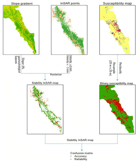
Figure 9.
Workflow of InSAR validation in GIS.
InSAR technology depends on radar coherent back scatterers, which are mainly found in built-up environments. However, in our case study, the landslide-susceptible areas are located on slopes, with a limited number of buildings and infrastructure. Additionally, active shallow landslides are characterized by the presence of vegetation, which is a main cause for signal decorrelation. Therefore, it was taken into account that the obtained InSAR deformation maps depict instability mainly in built-up areas, where the phenomenon is related to subsidence and uplift processes, which are in most cases caused by human impact, such as groundwater exploitation and construction works.
Points found on horizontal surfaces displaying velocities higher than +2 mm/yr in the sensor LOS (line of sight) were assumed to correspond to subsidence or uplift on a vertical direction and attributed to other tectonically driven processes. In order to eliminate the instability that is unrelated to landslides, the InSAR points found on horizontal and quasi-horizontal surfaces are discarded, starting from the point that landslides develop on slopes. For this purpose, all InSAR points located on areas with a slope gradient lower than 3% were eliminated from the analysis. The calculation of the slope gradient in the study area was based on a 1 m spatial resolution Lidar DEM resampled to 10 m resolution to match the spatial distribution of the InSAR points. A geomorphological map was applied to discard all InSAR points located along the river meadow and terrace treats. This procedure drastically reduced the number of available InSAR points derived from each orbit, decreasing the density of InSAR points from approximately 850 points/km2 to 120 points/km2 in the study area.
The unstable InSAR points from images obtained from both orbits are selected by imposing a threshold of stability between −2 mm/yr and 2 mm/yr, respectively, considering the InSAR results accuracy of ± 0.4 mm/yr and the assumption that movement lower than 2 mm/yr can be associated with stability. Points that display velocities outside the stability interval are associated with potential slope failure. By applying this binary classification, two InSAR deformation maps at 20 m resolution with stable/unstable condition classes are generated. The stability condition classes derived from each orbit were then merged into a single map containing InSAR-derived stable/unstable conditions. The susceptibility map is also classified into stable/unstable condition classes by merging the unstable and quasi-unstable classes into one singular class and resampling the data to a 20 m resolution raster. The two binary maps are then spatially cross correlated to derive the accuracy of the susceptibility map. In order to predict the ongoing landslides as indicated by InSAR and assess the correspondence between all defined classes, we present a confusion matrix in Table 4.
Table 4.
Confusion matrix for assessing the deterministic results accuracy relative to the InSAR-derived ground movement.
The comparison between InSAR and the susceptibility map reveals that the susceptibility analysis is able to predict more than 22% of the active landslides identified by InSAR (Table 4). This result is also conditioned by the constraint of back scatterers in coherent areas. In our view, most of the 78% missed ongoing displacements assemble all kind of ground movements, not only landslides (for example human impacts such as ground water extraction). As expected, the highest accuracy is obtained for the estimation of stable areas, which the deterministic map detected with an accuracy of around 82%.
7. Discussions and Conclusions
In this study, we combine classic and modern methodologies and their cross-validation in order to obtain a reliable landslide susceptibility map. The relative probability for spatial occurrence of mass movements is derived from the computation of the SF based on the geotechnical properties of slope materials. The most important geotechnical predictors for slope failure are cohesion, unit weight and friction angle. The trigger specific for the Subcarpathian study area is the rise in groundwater table, as a result of water infiltration during heavy rainfall episodes. Therefore, our landslide susceptibility map is valid under slope saturation conditions. In the Carpathian area, the most important characteristic of the lithology is the hardness of the rock, hence the values of cohesion and unit weight are high, and the values of friction angles are low. For this reason, even if we increase wetting conditions, the overall effect in terms of slope failure is negligible. Moreover, the mountain area of the Prahova Valley, characterized by flysch formations, is still well-forested, and more susceptible to deep-seated landslides. Old landslides located under forest are present, and this might affect our ability to capture all dynamic patterns of slope processes.
On the other hand, in the Subcarpathians, the rocks are soft, with alternating permeable/impermeable layers that trigger slope failure both in saturated and unsaturated conditions. For these soft rocks, cohesion and unit weight values are low, but friction angle values are higher compared to the mountain area. Increases in the water content of soil also increase the friction angle, thus the saturated condition has a much higher influence in slope failure. Since the Subcarpathian Prahova Valley is much more inhabited than the Carpathian area, an additional underground water source from water sewage spill and wastewater might cause higher landslide susceptibility classes.
The study reveals that in the Subcarpathians, the Breaza syncline, which is filled with a succession of Miocene clays, marls and sandstones, represents the most susceptible area and records the highest density of shallow-to-medium deep landslides affecting the overburden and a small part of the bedrock [8,35]. Some variations in type, size and orientation of landslides are induced by local strata gradients and the presence of faults. The pattern for future landslides is controlled by two morphological alignments: the continuous slope of the second terrace and the glacis of the upper third and fourth terraces.
In the hilly areas, landslides develop in relation to the length of the slope. On the second terrace slope, larger landslides are embedded on the southern flank of the syncline, forming amphitheater-shaped landslide heads. On the northern wing of the syncline, where Brebu conglomerates outcrop, there are shallower, stabilized and drained landslides. Overland flows become prevalent here, because of impermeable rocks [8].
Results are validated using a statistical approach and InSAR.
Although the infinite slope stability model applied in this study is influenced by uncertainties in measured geotechnical characteristics, the validation assessment and InSAR approach revealed a good performance in reproducing the observed landslide areas in the Subcarpathian reach of the Prahova Valley. In this hilly region, landslides are found in unstable and critical predicted areas, and the statistical validation of modelling results shows a good predictive capacity. For those areas with higher coherence for the radar signal, the SBAS-InSAR technique provided a good confirmation of slope dynamics, proving to be an adequate tool for landslide analysis.
The almost 23% of spatial overlay between the deterministic susceptibility map and the SBAS-InSAR ground deformation map is a result heavily conditioned by the presence of back scatterers. This result represents mostly areas characterized by regressive-developing scarps in the built-up areas or captures the presence of man-made features located on unstable slopes. The result of the validation for a potentially extreme scenario through InSAR is suited for revealing the slow ongoing movements in their initial developing state, with all the limitations imposed by the presence of signal coherent areas. Our SF map represents the probability of the occurrences for future landslides. The absence of movements detectable by InSAR for over 80% of the stable areas indicated as landslide-susceptible does not necessarily imply that these areas will not be affected by landslides in the future.
In order to improve our classic deterministic analysis, the susceptibility map is updated by integrating it with InSAR-detected instabilities. The areas defined as stable, quasi-unstable or unstable in the deterministic map are updated to a confirmed instability class if InSAR technique detects active movement (Figure 10).
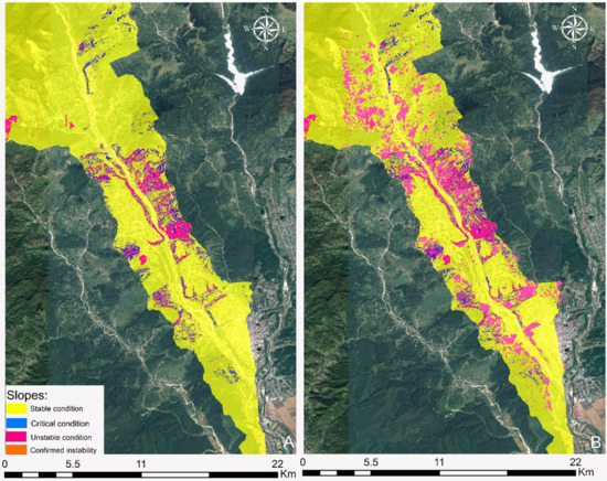
Figure 10.
The susceptibility map (A) and the updated susceptibility map (B). The areas defined as stable, quasi-unstable or unstable in the deterministic map were updated to a confirmed instability class, if InSAR techniques detected corresponding active movement. Map created in QGIS3 software Base map: Landsat 8 scene from 20 August 2019, downloaded from Earth Resources Observation and Science (EROS) Center, USGS.
Since built-up areas show the best candidates for radar scatterers, the proposed methodology brings the most reliable results for landslide detection in populated environments, while capabilities of the current satellite SAR sensors are still limited in natural, highly vegetated areas. Several authors have proposed improved algorithms that increase coherence in natural areas (SqueeSAR) [82,83,84], but in the current study area, the presence of high vegetation causes a temporal decorrelation of the C-band signal regardless of the selected method. However, we show that the use of InSAR for monitoring slow-developing landslides affecting inhabited and constructed areas is meaningful and produces satisfactory results. Considering that the study area presents good reflectivity and coherence, the proposed technique offers a highly accurate estimation of ground displacement on sliding slopes.
The characteristics of each method makes them more suitable for different types of environments. While InSAR is able to confirm active movements in built-up environments, the deterministic method focuses on vegetated slopes that limit the applicability of the remote sensing technique. Therefore, refined maps of landslide susceptibility obtained by integrating these two complementary methods offer a more complete view of an area of interest, and enhance landslide susceptibility estimations in areas with existing infrastructure and buildings, or where future key infrastructure projects are planned.
Author Contributions
Conceptualization, research design, deterministic approach, validation, writing—original draft preparation, I.A.; InSAR; writing—review and editing, M.G.; geological investigation and analysis, G.C.S. All authors have read and agreed to the published version of the manuscript.
Funding
This research was funded by the Romanian Space Agency (ROSA) through The Research, Development and Innovation STAR Programme—Space Technology and Advanced Research, GEOVIEW project, grant number 146/2016, having I. Armaş as Principal Investigator.
Institutional Review Board Statement
Not applicable.
Informed Consent Statement
Not applicable.
Data Availability Statement
The data generated and studied in this article can be obtained upon request to the principal author.
Acknowledgments
Geotechnical parameters used in this study are provided through written agreements with the following private companies: S.C. FORMIN S.A., S.C. SEARCH CORPORATION S.R.L. and SIXSENSE ROMÂNIA.
Conflicts of Interest
The authors declare no conflict of interest.
References
- Varnes, D.J. Slope movement types and processes. In Special Report 176: Landslides: Analysis and Control; Schuster, R.L., Krizek, R.J., Eds.; Transportation and Road Research Board, National Academy of Science: Washington, DC, USA, 1978; pp. 11–33. [Google Scholar]
- Geografia României, I. Geografi a Fizică (Geography of Romania, I. Physical Geography); Edit. Academiei: Bucureşti, Romania, 1983; pp. 171–194. (In Romanian) [Google Scholar]
- Bălteanu, D. Romania. In Geomorphological Hazards of Europe; Embelton, C., Embelton-Hamann, C., Eds.; Elsevier: Amsterdam, The Netherlands, 1997; pp. 409–427. [Google Scholar]
- Micu, M.; Bălteanu, D. Landslide hazard assessment in the Bend Carpathians and Subcarpathians, Romania. Z. Geomorphol. 2009, 53 (Suppl. 3), 49–64. [Google Scholar] [CrossRef]
- Micu, M.; Sima, M.; Bălteanu, D.; Micu, D.; Dragotă, C.; Chendeş, V. A multi-hazard assessment in the Curvature Carpathians of Romania. In Mountain Risks: Bringing Science to Society; Malet, J.-P., Glade, T., Casagli, N., Eds.; CERG Editions: Strasbourg, Germany, 2010; pp. 11–18. [Google Scholar]
- Bălteanu, D.; Jurchescu, M.; Surdeanu, V.; Ionita, I.; Goran, C.; Urdea, P.; Rădoane, M.; Rădoane, N.; Sima, M. Recent landform evolution in the Romanian Carpathians and Pericarpathian Regions. In Recent Landform Evolution: The Carpatho–Balkan–Dinaric Region; Lóczy, D., Stankoviansky, M., Kotarba, A., Eds.; Springer Geography: Berlin/Heidelberg, Germany, 2012. [Google Scholar] [CrossRef]
- Bălteanu, D. The importance of mass movements in the Romanian Subcarpathians. Z. Fur Geomorphol. 1986, 58, 173–190. [Google Scholar]
- Armaş, I.; Damian, R.; Sandric, I.; Osaci-Costache, G. Vulnerabilitatea Versantilor Subcarpatici la Alunecari de Teren (Valea Prahovei); Editura Fundatiei Romania de Maine: Bucharest, Romania, 2003. [Google Scholar]
- Surdeanu, V. La repartition des glissements de terrain dans le Carpates Orientales (zone du flysch). Geogr. Fis. Din. Quat. 1996, 19, 265–271. [Google Scholar]
- Wieczorek, G.F. Preparing a detailed landslide-inventory map for hazard evaluation and reduction. Bull. Assoc. Eng. Geol. 1984, 21, 337–342. [Google Scholar] [CrossRef]
- Van Westen, C.J.; Castellanos, E.; Kuriakose, S.L. Spatial data for landslide susceptibility, hazard, and vulnerability assessment: An overview. Eng. Geol. 2008, 102, 112–131. [Google Scholar] [CrossRef]
- Brabb, E.E. Innovative approaches to landslide hazard and risk mapping. In Proceedings of the 4th International Symposium on Landslides, Toronto, ON, Canada, 16–21 September 1984; Volume 1, pp. 307–324. [Google Scholar]
- Van Westen, J. Landslide Hazard. Zonation: A Review with Examples from the Colombian Andes; Price, M.F., Heywood, D.I., Eds.; Taylor and Francis: London, UK, 1994; pp. 135–165. [Google Scholar]
- Guzzetti, F.; Carrara, A.; Cardinali, M.; Reichenbach, P. Landslide hazard evaluation: A review of current techniques and their application in a multi-scale study, Central Italy. Geomorphology 1999, 31, 181–216. [Google Scholar] [CrossRef]
- Carson, M.A.; Kirkby, M.J. Hillslope Form and Process; Cambridge University Press: London, UK, 1972. [Google Scholar]
- Crozier, M.J. Landslides: Causes Consequences and Environment; Croom Helm: London, UK, 1986. [Google Scholar]
- Aleotti, P.; Chowdhury, R. Landslide hazard assessment: Summary review and new perspectives. Bull. Eng. Geol. Environ. 1999, 58, 21–44. [Google Scholar] [CrossRef]
- Duncan, J.M.; Wright, S.G. Soil Strength and Slope Stability; Wiley: Hoboken, NJ, USA, 2005. [Google Scholar]
- Van Westen, C.J. The modelling of landslide hazards using GIS. Surv. Geophys. 2000, 21, 241–255. [Google Scholar] [CrossRef]
- Guzzetti, F. Landslide Hazard and Risk Assessment. Ph.D. Thesis, University of Bonn, Bonn, Germany, 2000. [Google Scholar]
- Van Westen, C.J.; Van Asch, T.W.J.; Soeters, R. Landslide hazard and risk zonation–Why is it still so difficult? Bull. Eng. Geol. Environ. 2006, 65, 167–184. [Google Scholar] [CrossRef]
- Van Westen, C.J.; Terlien, T.J. An approach towards deterministic landslide hazard analysis in GIS. A case study from Manizales (Colombia). Earth Surf. Process. Landf. 1996, 21, 853–868. [Google Scholar] [CrossRef]
- Sharma, S. Slope Stability Concepts. In Slope Stability and Stabilization Methods; Abramson, L.W., Lee, T.S., Sharma, S., Boyce, G.M., Eds.; John Wiley & Sons, Inc.: New York, NY, USA, 2002; pp. 329–461. [Google Scholar]
- Cruden, D.M.; Varnes, D.J. Landslides: Investigation and mitigation. Chapter 3-Landslide types and processes. In Transportation Research Board Special Report; National Academy Press: Washington, DC, USA, 1996; p. 247. [Google Scholar]
- Lu, N.; Godt, J.W. Hillslope Hydrology and Stability; Cambridge University Press: Cambridge, UK, 2013. [Google Scholar]
- Dietrich, W.E.; Bellugi, D.; De Asua, R. Validation of the shallow landslide model, SHALSTAB, for forest management. In Land Use and Watersheds: Human Influence on Hydrology and Geomorphology in Urban and Forest Areas; Wigmosta, M.S., Burges, S.J., Eds.; American Geophysical Union: Washington, DC, USA, 2001; pp. 195–227. [Google Scholar]
- Borga, M.; Dalla Fontana, G.; Gregoretti, C.; Marchi, L. Assessment of shallow landsliding by using a physically based model of hillslope stability. Hydrol. Process. 2002, 16, 2833–2851. [Google Scholar] [CrossRef]
- Huang, J.-C.; Kao, S.-J.; Hsu, M.-L.; Liu, Y.-A. Influence of Specific Contributing Area algorithms on slope failure prediction in landslide modeling. Nat. Hazards Earth Syst. Sci. 2007, 7, 781–792. [Google Scholar] [CrossRef]
- Frattini, P.; Crosta, G.B.; Fusi, N.; Dal Negro, P. Shallow landslides in pyroclastic soils: A distributed modelling approach for hazard assessment. Eng. Geol. 2004, 73, 277–295. [Google Scholar] [CrossRef]
- Rosso, R.; Rulli, M.C.; Vannucchi, G. A physically based model for the hydrologic control on shallow landsliding. Water Res. 2006, 42, 6410. [Google Scholar] [CrossRef]
- Godt, J.W.; Baum, R.L.; Savage, W.Z.; Salciarini, D.; Schulz, W.H.; Harp, E.L. Transient deterministic shallow landslide modeling: Requirements for susceptibility and hazard assessments in a GIS framework. Eng. Geol. 2008, 102, 214–226. [Google Scholar] [CrossRef]
- D’Amato Avanzi, G.; Falaschi, F.; Giannecchini, R.; Puccinelli, A. Soil slip susceptibility assessment using mechanical-hydrological approach and GIS techniques: An application in the Apuan Alps (Italy). Nat. Hazards 2009, 50, 591–603. [Google Scholar] [CrossRef]
- Ho, J.Y.; Lee, K.T.; Chang, T.C.; Wang, Z.Y.; Liao, Y. Influences of spatial distribution of soil thickness on shallow landslide prediction. Eng. Geol. 2012, 124, 38–46. [Google Scholar] [CrossRef]
- Alvioli, M.; Guzzetti, F.; Rossi, M. Scaling properties of rainfall induced landslides predicted by a physically based model. Geomorphology 2014, 213, 38–47. [Google Scholar] [CrossRef]
- Armaş, I.; Vartolomei, F.; Stroia, F.; Brasovanu, L. Landslide susceptibility deterministic approach using geographical information systems: Application to Breaza city, Romania. Nat. Hazards 2014, 70, 995–1017. [Google Scholar] [CrossRef]
- Bürgmann, R.; Rosen, P.A.; Fielding, E.J. Synthetic aperture radar interferometry to measure Earth’s surface topography and its deformation. Annu. Rev. Earth Planet. Sci. 2000, 28, 169–209. [Google Scholar] [CrossRef]
- Colesanti, C.; Wasowski, J. Investigating landslides with space-borne Synthetic Aperture Radar (SAR) interferometry. Eng. Geol. 2006, 88, 173–199. [Google Scholar] [CrossRef]
- Dammert, P.B. Accuracy of INSAR measurements in forested areas. In Proceedings of the Fringe 96 Workshop, Zurich, Switzerland, 30 September–2 October 1996; Volume 406, pp. 37–45. [Google Scholar]
- Ferretti, A.; Savio, G.; Barzaghi, R.; Borghi, A.; Musazzi, S.; Novali, F.; Prati, C.; Rocca, F. Submillimeter accuracy of InSAR time series: Experimental validation. IEEE Trans. Geosci. Remote Sens. 2007, 45, 1142–1153. [Google Scholar] [CrossRef]
- Torres, R.; Snoeij, P.; Geudtner, D.; Bibby, D.; Davidson, M.; Attema, E.; Potin, P.; Rommen, B.; Floury, N.; Brown, M.; et al. GMES Sentinel-1 mission. Remote Sens. Environ. 2012, 120, 9–24. [Google Scholar] [CrossRef]
- Ferretti, A.; Prati, C.; Rocca, F. Non-linear subsidence rate estimation using permanent scatterers in differential SAR interferometry. IEEE Trans. Geosci. Remote Sens. 2000, 38, 2202–2212. [Google Scholar] [CrossRef]
- Ferretti, A.; Prati, C.; Rocca, F. Permanent scatterers in SAR interferometry. IEEE Trans. Geosci. Remote Sens. 2001, 39, 8–20. [Google Scholar] [CrossRef]
- Farina, P.; Colombo, D.; Fumagalli, A.; Marks, F.; Moretti, S. Permanent Scatterers for landslide investigations: Outcomes from the ESA-SLAM project. Eng. Geol. 2006, 88, 200–217. [Google Scholar] [CrossRef]
- Motagh, M.; Wetzel, H.-U.; Roessner, S.; Kaufmann, H. A TerraSAR-X InSAR study of landslides in southern Kyrgyzstan, central Asia. Remote Sens. Lett. 2013, 4, 657–666. [Google Scholar] [CrossRef]
- Hölbling, D.; Füreder, P.; Antolini, F.; Cigna, F.; Casagli, N.; Lang, S. A semi-automated object-based approach for landslide detection validated by persistent scatterer interferometry measures and landslide inventories. Remote Sens. 2012, 4, 1310–1336. [Google Scholar] [CrossRef]
- Righini, G.; Pancioli, V.; Casagli, N. Updating landslide inventory maps using Persistent Scatterer Interferometry (PSI). Int. J. Remote Sens. 2012, 33, 2068–2096. [Google Scholar] [CrossRef]
- Berardino, P.; Fornaro, G.; Lanari, R.; Sansosti, E. A new algorithm for surface deformation monitoring based on small baseline differential SAR interferometry. IEEE Aerosp. Electron. 2002, 40, 2375–2383. [Google Scholar]
- Zhao, C.; Zhong, L.; Zhang, Q.; de La Fuente, J. Large-area landslide detection and monitoring with ALOS/PALSAR imagery data over Northern California and Southern Oregon, USA. Remote Sens. Environ. 2012, 124, 348–359. [Google Scholar] [CrossRef]
- Liu, P.; Li, Z.; Hoey, T.; Kincal, C.; Zhang, J.; Zeng, Q.; Muller, J.P. Using advanced InSAR time series techniques to monitor landslide movements in Badong of the Three Gorges region. China. Int. J. Appl. Earth Obs. Geoinf. 2013, 21, 253–264. [Google Scholar] [CrossRef]
- Cascini, L.; Fornaro, G.; Peduto, D. Advanced low-and full-resolution DInSAR map generation for slow-moving landslide analysis at different scales. Eng. Geol. 2010, 112, 29–426. [Google Scholar] [CrossRef]
- Cascini, L.; Peduto, D.; Pisciotta, G.; Arena, L.; Ferlisi, S.; Fornaro, G. The combination of DInSAR and facility damage data for the updating of slow-moving landslide inventory maps at medium scale. Nat. Hazards Earth Syst. Sci. 2013, 13, 1527. [Google Scholar] [CrossRef]
- Bateson, L.; Cigna, F.; Boon, D.; Sowter, A. The application of the Intermittent SBAS (ISBAS) InSAR method to the South Wales Coalfield, UK. Int. J. Appl. Earth Obs. Geoinf. 2015, 34, 249–257. [Google Scholar] [CrossRef]
- Bianchini, S.; Cigna, F.; Righini, G.; Proietti, C.; Casagli, N. Landslide hotspot mapping by means of persistent scatterer interferometry. Environ. Earth Sci. 2012, 67, 1155–1172. [Google Scholar] [CrossRef]
- Tantianuparp, P.; Shi, X.; Zhang, L.; Balz, T.; Liao, M. Characterization of landslide deformations in three gorges area using multiple InSAR data stacks. Remote Sens. 2013, 5, 2704–2719. [Google Scholar] [CrossRef]
- Bozzano, F.; Mazzanti, P.; Perissin, D.; Rocca, A.; De Pari, P.; Discenza, M.E. Basin scale assessment of landslides geomorphological setting by advanced InSAR analysis. Remote Sens. 2017, 9, 267. [Google Scholar] [CrossRef]
- Dai, K.; Li, Z.; Tomás, R.; Liu, G.; Yu, B.; Wang, X.; Stockamp, J. Monitoring activity at the Daguangbao mega-landslide (China) using Sentinel-1 TOPS time series interferometry. Remote Sens. Environ. 2016, 186, 501–513. [Google Scholar] [CrossRef]
- Intrieri, E.; Raspini, F.; Fumagalli, A.; Lu, P.; Del Conte, S.; Farina, P.; Allievi, J.; Ferretti, A.; Casagli, N. The Maoxian landslide as seen from space: Detecting precursors of failure with Sentinel-1 data. Landslides 2018, 15, 123–133. [Google Scholar] [CrossRef]
- Béjar-Pizarro, M.; Notti, D.; Mateos, R.M.; Ezquerro, P.; Centolanza, G.; Herrera, G.; Bru, G.; Sanabria, M.; Solari, L.; Duro, J.; et al. Mapping vulnerable urban areas affected by slow-moving landslides using Sentinel-1 InSAR data. Remote Sens. 2017, 9, 876. [Google Scholar] [CrossRef]
- Bardi, F.; Raspini, F.; Ciampalini, A.; Kristensen, L.; Rouyet, L.; Lauknes, T.; Frauenfelder, R.; Casagli, N. Space-borne and ground-based InSAR data integration: The Åknes test site. Remote Sens. 2016, 8, 237. [Google Scholar] [CrossRef]
- Necula, N.; Niculiță, M.; Tessari, G.; Floris, M. InSAR analysis of Sentinel-1 data for monitoring landslide displacement of the north-eastern Copou hillslope, Iași city, Romania. In Proceedings of the Romanian Geomorphology Symposium, Iași, Romania, 11–14 May 2017; Volume 1, pp. 85–88. [Google Scholar]
- Armaş, I.; Gogoașe Nistoran, D.; Osaci-Costache, G.; Brașoveanu, L. Morpho-Dynamic Evolution Patterns of Subcarpathian Prahova River (Romania). Catena 2013, 100, 83–99. [Google Scholar] [CrossRef]
- Ştefănescu, M.; Mărunţeanu, M. Age of the Doftana Molasse, Dări de Seamă ale Şedinţelor; Institututl Geologic al Romaniei: Bucuresti, Romania, 1980; Volume LXV/4, pp. 169–182. [Google Scholar]
- Săndulescu, M. Geotectonica României; Editura Tehnică: Bucharest, Romania, 1984. [Google Scholar]
- Ştefănescu, M. Stratigraphy and structure of cretaceous and paleogene flysch deposits between Prahova and Ialomiţa valleys. Rom. J. Tecton. Reg. Geol. 1995, 76, 3–49. [Google Scholar]
- Armaş¸, I. Bazinul Hidrografic Doftana. Studiu de Geomorfologie; Ed. Enciclopedică: Bucharest, Romania, 1999; p. 240. [Google Scholar]
- Armaş, I.; Damian, R.; Stroia, F. The Vulnerability of Scarps Caused by Anthropic Impact. Case Study: The Breaza Terrace Scarp-The Prahova Valley. Present Environ. Sustain. Dev. 2007, 1, 179–191. [Google Scholar]
- Armaş, I.; Damian, R.; Sandric, I. Landslides in the M. Căproiu St.- Eternității St. perimeter, town of Breaza. Rev. Geomorfol. 2004, VI, 61–71. [Google Scholar]
- Armaş, I.; Damian, R. Evolutive Interpretation of the Landslides from the Miron Căproiu Street Scarp (Eternităţii Street– V. Alecsandri Street)–Breaza Town. Rev. Geomorfol. 2006, VIII, 65–72. [Google Scholar]
- Beek, L.P.H. Van Assessment of the Influence of Changes in Landuse and Climate on Landslide Activity in a Mediterranean Environment. Ph.D. Thesis, Utrecht University, Utrecht, Germany, 2002. [Google Scholar]
- Mergili, M.; Marchesini, I.; Alvioli, M.; Metz, M.; Schneider-Muntau, B.; Rossi, M.; Guzzetti, F. A strategy for GIS-based 3-D slope stability modelling over large areas. Geosci. Model. Dev. 2014, 7, 2969–2982. [Google Scholar] [CrossRef]
- Brunsden, D.; Prior, D.B. Slope Stability; Wiley: Hoboken, NJ, USA, 1984; p. 620. [Google Scholar]
- Ardeleanu, L.; Leydecker, G.; Bonjer, K.P.; Busche, H.; Kaiser, D.; Schmitt, T. Probabilistic seismic hazard map for Romania as a basis for a new building code. Nat. Hazards Earth Syst. Sci. 2005, 5, 679–684. [Google Scholar] [CrossRef]
- Mărmureanu, G.; Cioflan, C.O.; Mărmureanu, A. New approach on seismic hazard isoseismal map for Romania. Rom. Rep. Phys. 2008, 60, 1123–1135. [Google Scholar]
- Costantini, M.; Rosen, P.A. A generalized phase unwrapping approach for sparse data. In Proceedings of the IEEE 1999 International Geoscience and Remote Sensing Symposium, Hamburg, Germany, 28 June–2 July 1999; Volume 1, pp. 267–269. [Google Scholar]
- Istrate, A. The role of the tectonic factor in the distribution of the landslides in the Carpathian flysch from the Ialomita basin. In Forum Geografic (No. 4); Department of Geography, University of Craiova: Craiova, Romania, 2005; p. 26. [Google Scholar]
- Sidle, R.C. Relative importance of factors influencing landsliding in coastal Alaska. In Proceedings of the 21st Annual Engineering, Geology and Soil Engineering Symposium, Moscow, ID, USA, 5–6 April 1984; University of Idaho: Idaho, Moscow, USA; pp. 311–325. [Google Scholar]
- Chang, H.; Kim, N.K. The evaluation and the sensitivity analysis of GIS-based landslide susceptibility models. Geosci. J. 2004, 8, 415–423. [Google Scholar] [CrossRef]
- Crosta, G.B.; Frattini, P. Distributed modelling of shallow landslides triggered by intense rainfall. Nat. Hazards Earth Syst. Sci. 2003, 3, 81–93. [Google Scholar] [CrossRef]
- Pratesi, F.; Tapete, D.; Terenzi, G.; Del Ventisette, C.; Moretti, S. Rating health and stability of engineering structures via classification indexes of InSAR Persistent Scatterers. Int. J. Appl. Earth Obs. Geoinf. 2015, 40, 81–90. [Google Scholar] [CrossRef]
- Chung, C.F.; Fabbri, A.G. Validation of spatial prediction models for landslide hazard mapping. Nat. Hazards 2003, 30, 451–472. [Google Scholar] [CrossRef]
- Vázquez-Selem, L.; Zinck, A.J. Modeling gully distribution on volcanic terrains in the Huasca area, central Mexico. ITC J. 1994, 3, 238–251. [Google Scholar]
- Zinck, J.A.; López, J.; Metternicht, G.I.; Shrestha, D.P.; Vázquez-Selem, L. Mapping and modelling mass movements and gullies in mountainous areas using remote sensing and GIS techniques. Int. J. Appl. Earth Obs. Geoinf. 2001, 3, 43–53. [Google Scholar] [CrossRef]
- Ferretti, A.; Fumagalli, A.; Novali, F.; Prati, C.; Rocca, F.; Rucci, A. A new algorithm for processing interferometric data-stacks: SqueeSAR. IEEE Trans. Geosci. Remote Sens. 2011, 49, 3460–3470. [Google Scholar] [CrossRef]
- Meisina, C.; Notti, D.; Zucca, F.; Ceriani, M.; Colombo, A.; Poggi, F.; Roccati, A.; Zaccone, A. The use of PSInSAR™ and SqueeSAR™ techniques for updating landslide inventories. In Landslide Science and Practice; Springer: Berlin/Heidelberg, Germany, 2013; pp. 81–87. [Google Scholar]


Publisher’s Note: MDPI stays neutral with regard to jurisdictional claims in published maps and institutional affiliations. |
© 2021 by the authors. Licensee MDPI, Basel, Switzerland. This article is an open access article distributed under the terms and conditions of the Creative Commons Attribution (CC BY) license (https://creativecommons.org/licenses/by/4.0/).