
Small Angle Scattering Intensity Measurement by an Improved Ocean Scheimpflug Lidar System


Abstract
1. Introduction
2. The Ocean Scheimpflug Lidar System
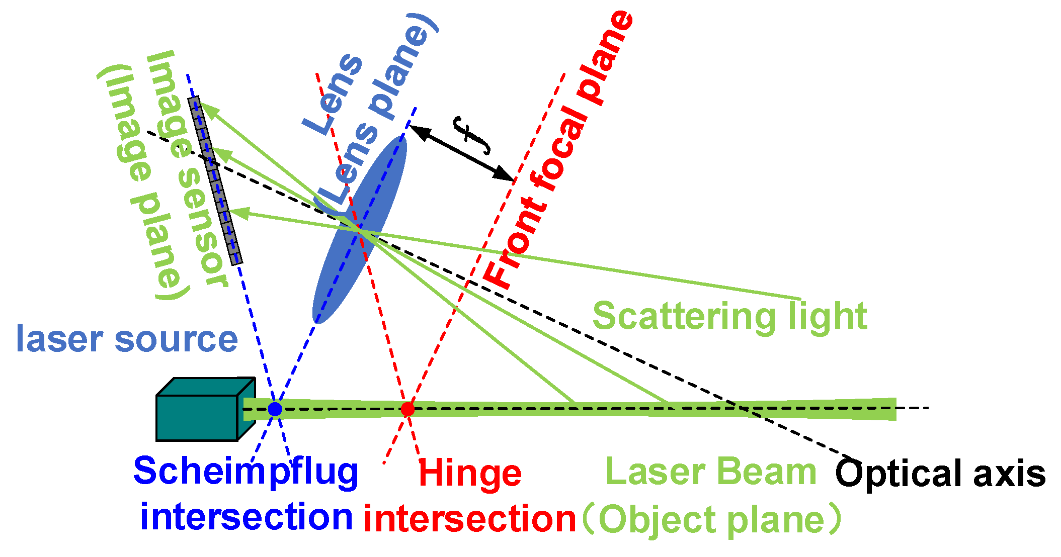
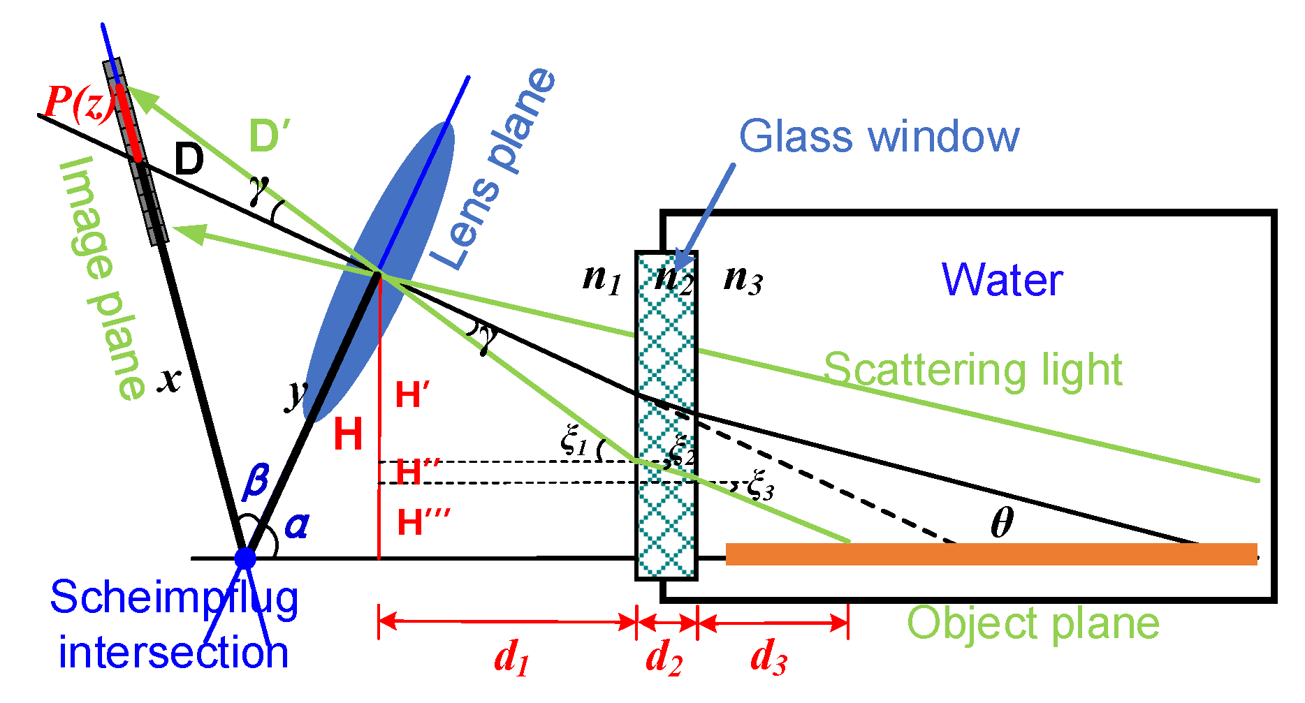
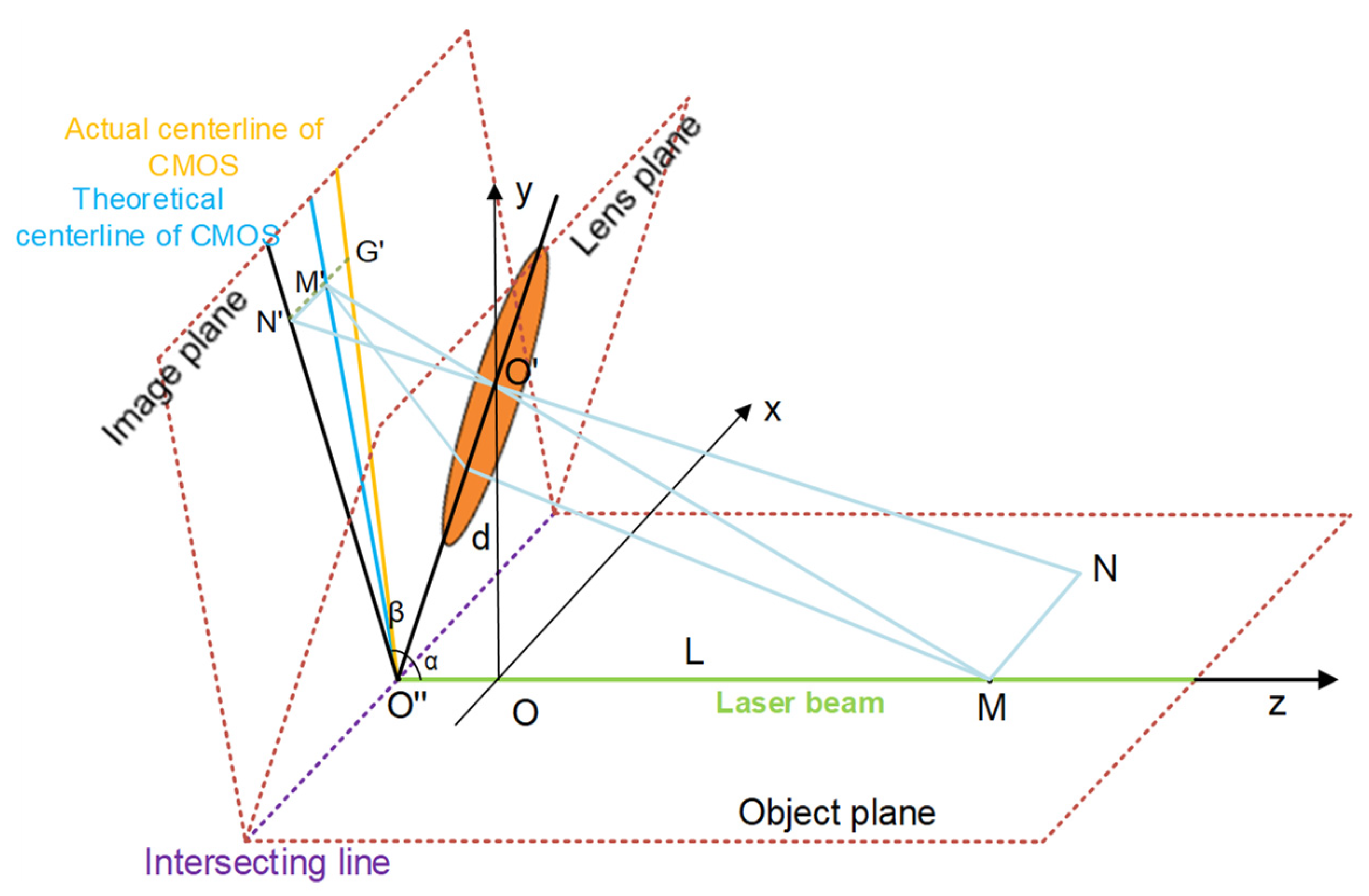
2.1. General Principle
2.2. Specifications of the Scheimpflug Lidar System
2.2.1. Transmitter
2.2.2. Receiver
2.2.3. Detector
3. Experiment and Methodology
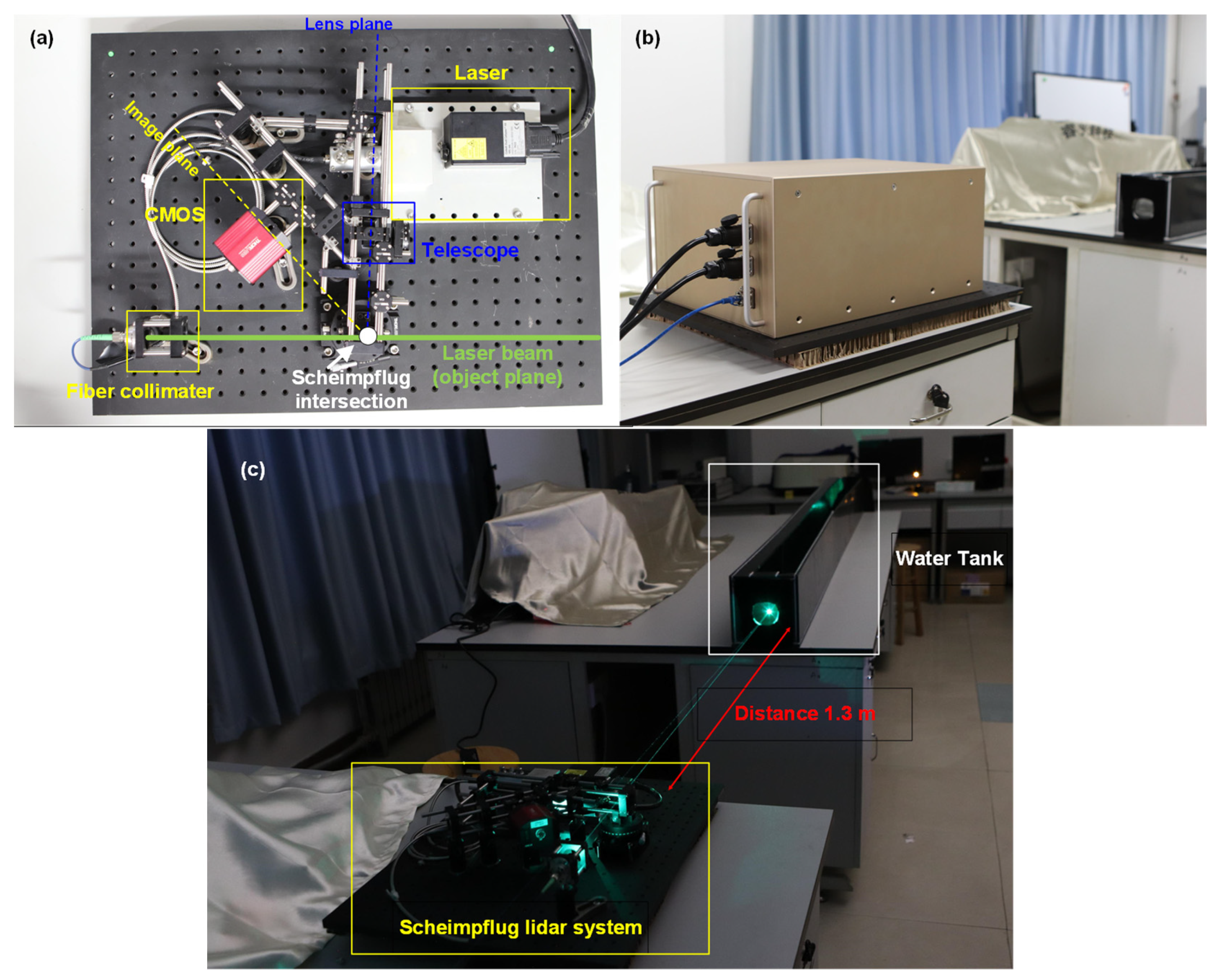
3.1. Experimental Setup
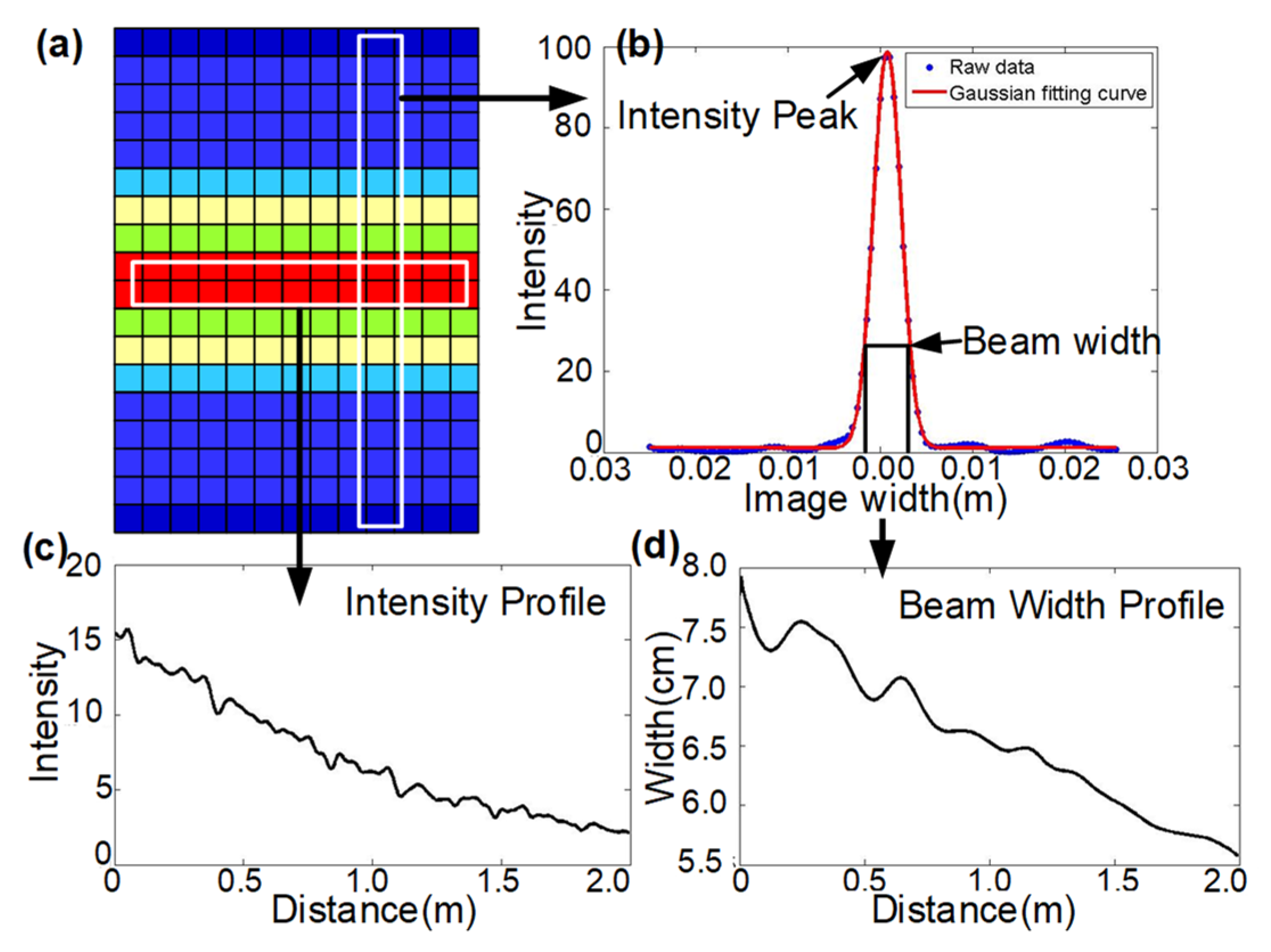
3.2. Imaging Processing
3.3. Monte Carlo Simulation
4. Results
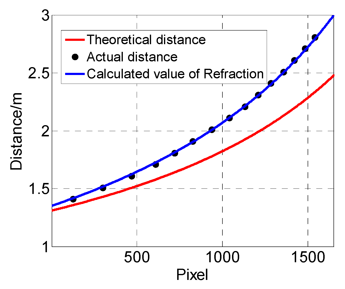
Validation
5. Discussions and Conclusions
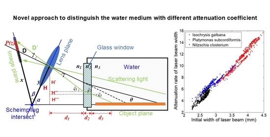
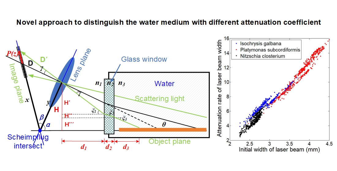
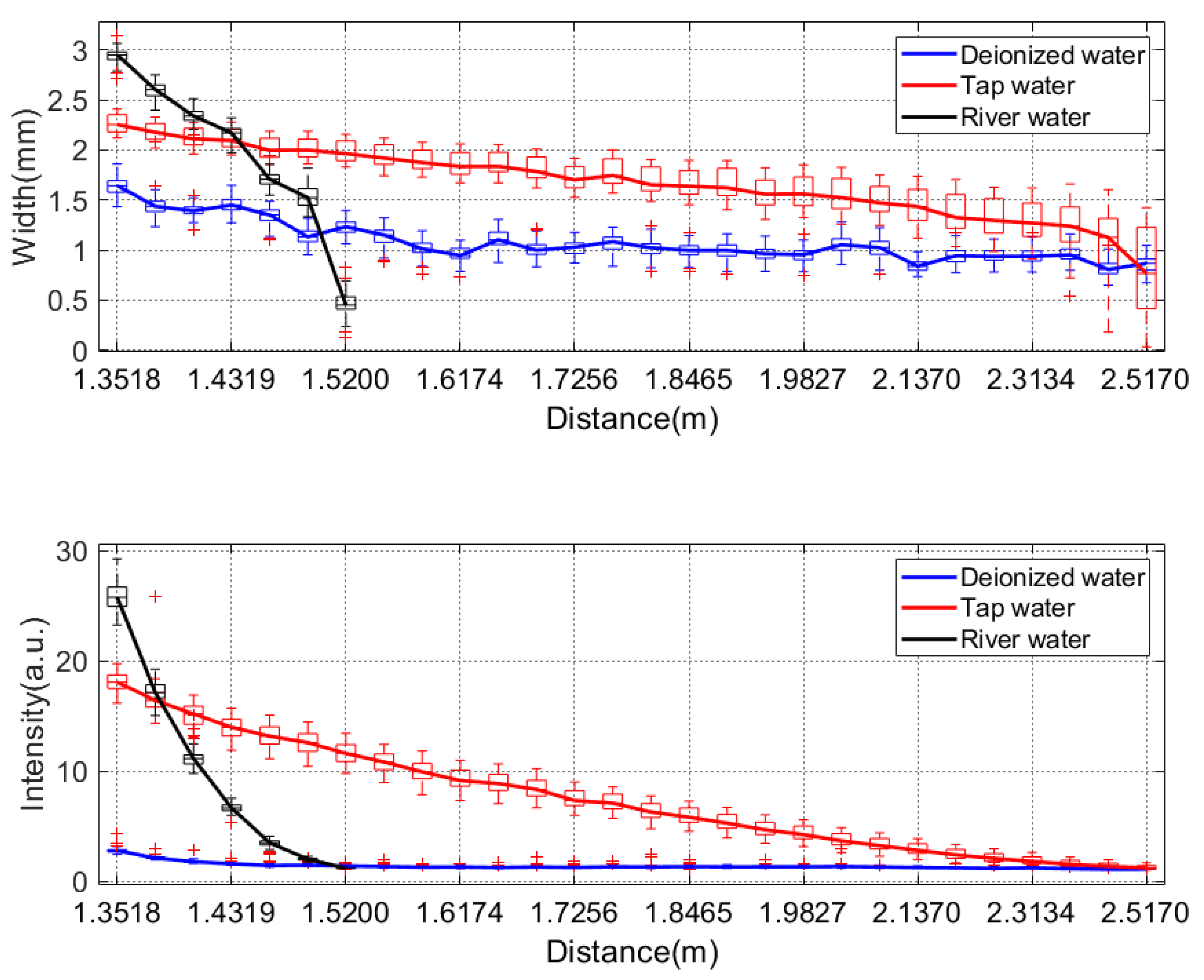
- A novel optical approach was developed to measure the scattering intensity and to quantify the characteristics of the suspended particles within small angles at backwards and distinguish water medium with different attenuation coefficients.
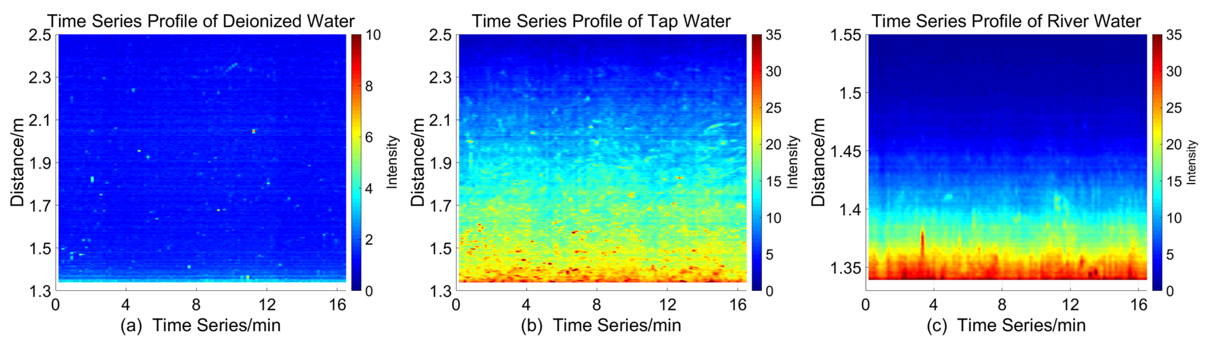
- The work aimed to verify the capability of the Scheimpflug system to distinguish different water mediums with different optical parameters.
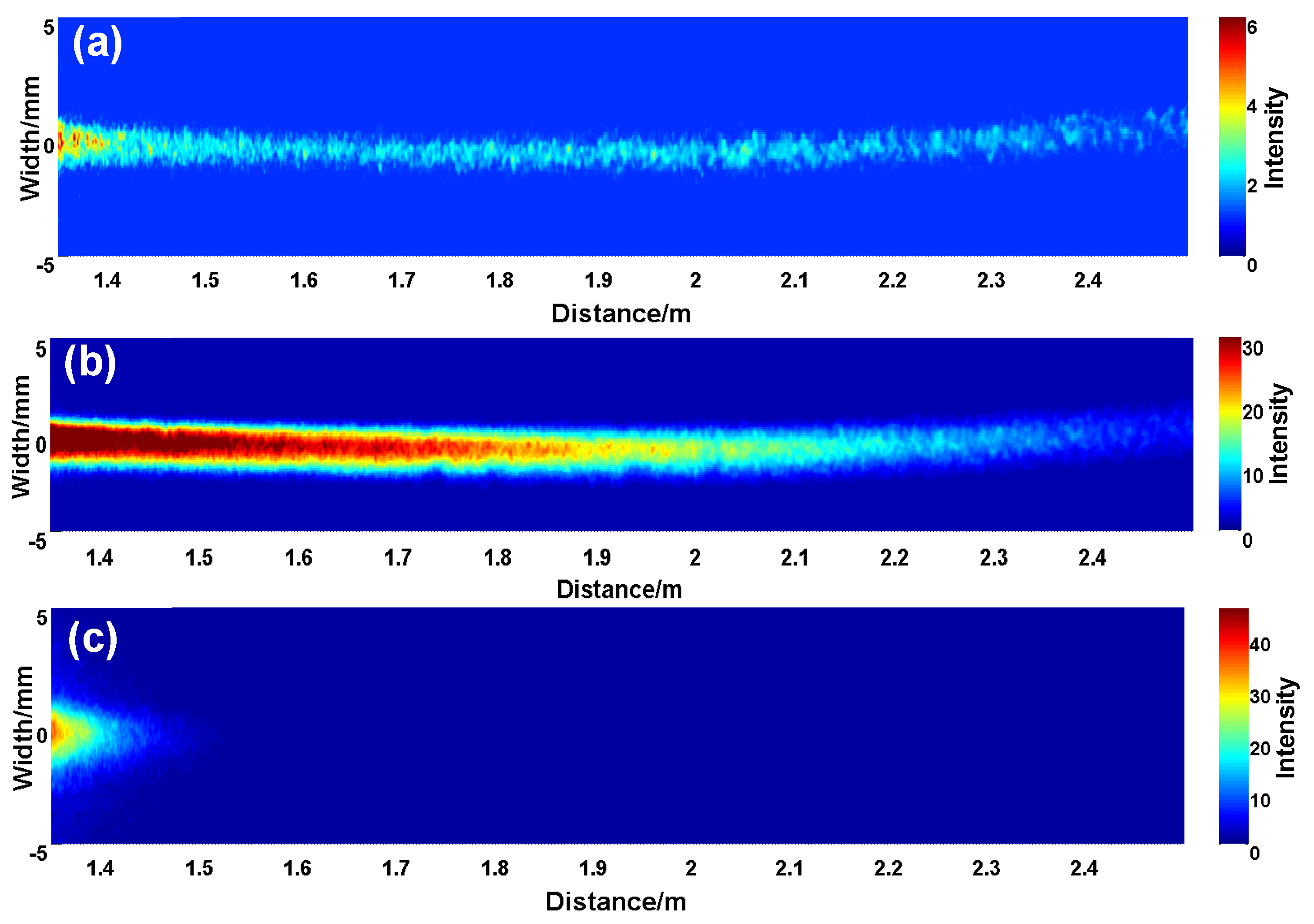
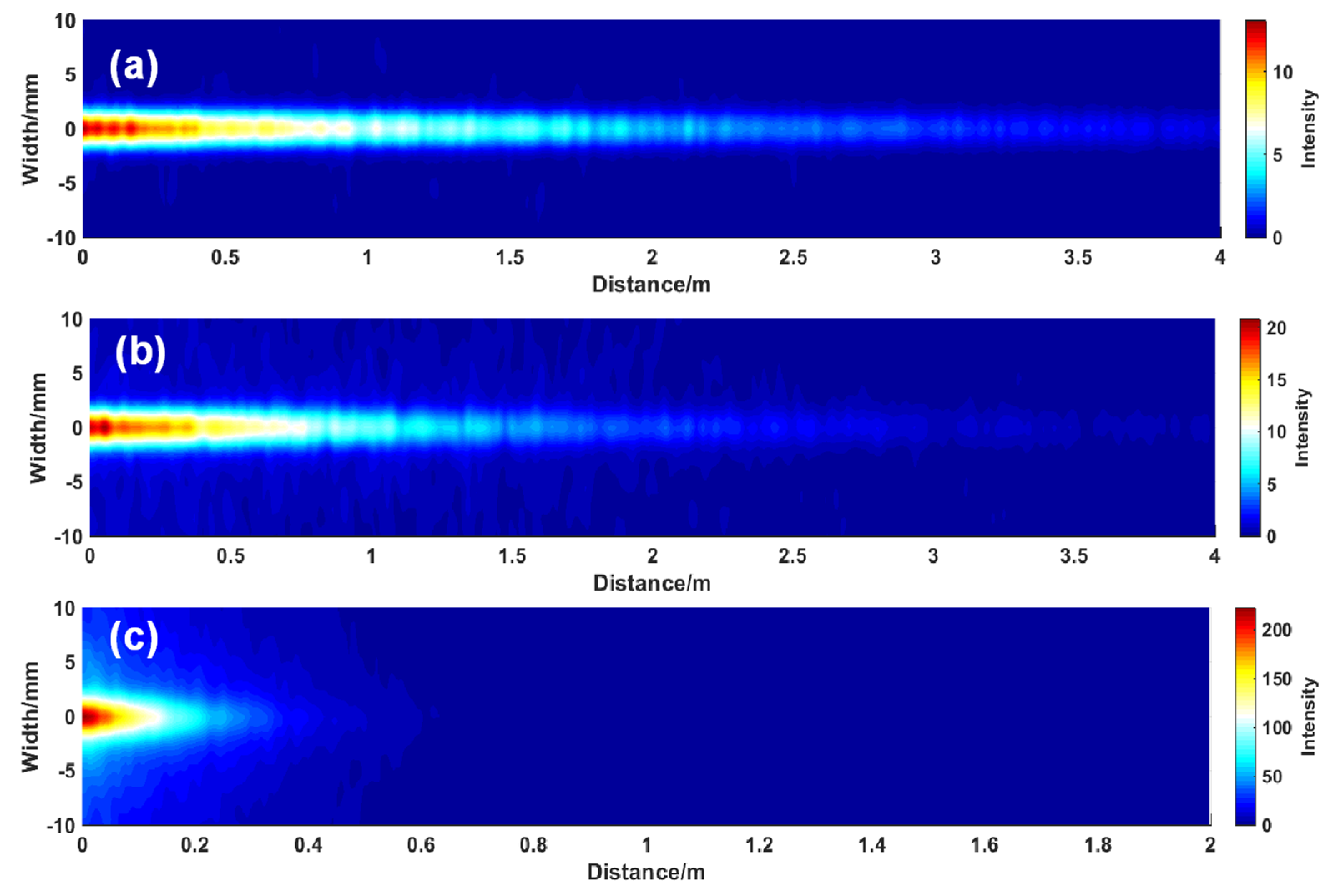
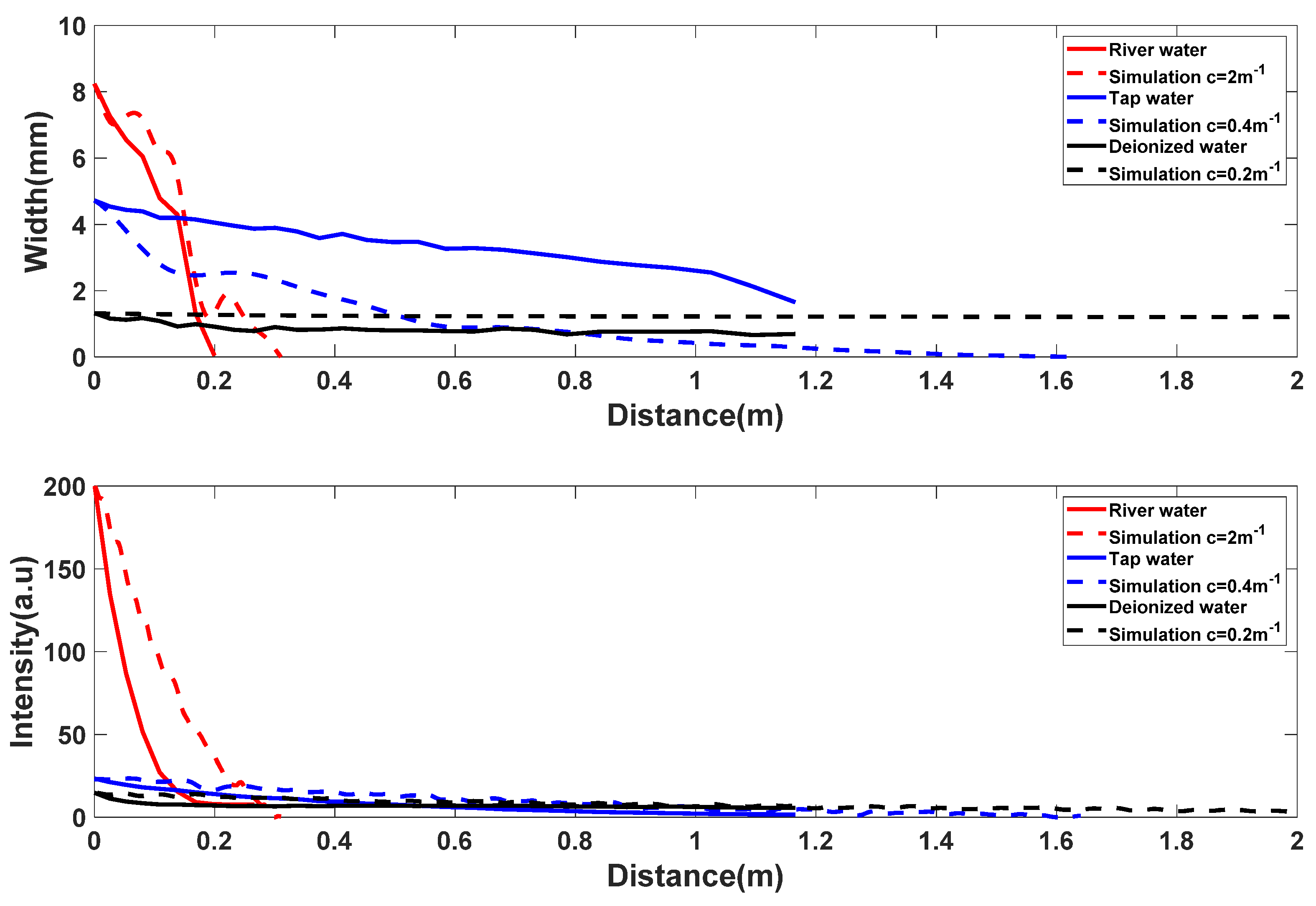
- Intensity-range maps simulated by the Monte Carlo methods under three different water mediums with different attenuation coefficients were developed.
Author Contributions
Funding
Institutional Review Board Statement
Informed Consent Statement
Data Availability Statement
Acknowledgments
Conflicts of Interest
Appendix A
Appendix B

Appendix C

References
- Soomets, T.; Uudeberg, K.; Jakovels, D.; Brauns, A.; Zagars, M.; Kutser, T. Validation and Comparison of Water Quality Products in Baltic Lakes Using Sentinel-2 MSI and Sentinel-3 OLCI Data. Sensors 2020, 20, 742. [Google Scholar] [CrossRef] [PubMed]
- Aguilar-Maldonado, J.A.; Santamaría-del-Ángel, E.; Gonzalez-Silvera, A.; Sebastiá-Frasquet, M.T. Detection of Phytoplankton Temporal Anomalies Based on Satellite Inherent Optical Properties: A Tool for Monitoring Phytoplankton Blooms. Sensors 2019, 19, 3339. [Google Scholar] [CrossRef]
- Milton, K.; Joao, A.L.; Cristina, M.B. Simultaneous measurements of Chlorophyll concentration by lidar, fluorometry, above-water radiometry, and ocean color MODIS images in the Southwestern Atlantic. Sensors 2009, 9, 528–541. [Google Scholar] [CrossRef]
- Michael, E.L.; Marlon, R.L. A new method for the measurement of the optical volume scattering function in the upper ocean. J. Atmos. Ocean. Technol. 2003, 20, 563–571. [Google Scholar] [CrossRef]
- Eric, R.; Norman, J.M. Inherent optical property estimation in deep waters. Opt. Express 2011, 19, 24986–25005. [Google Scholar] [CrossRef]
- David, R.L. Remote sensing of bottom reflectance and water attenuation parameters in shallow water using aircraft and Landsat data. Int. J. Remote Sens. 1981, 2, 71–82. [Google Scholar] [CrossRef]
- Ina, L.; Fethi, B.; Charles, T.; Rüdiger, R.; David, B.; Alex, N.; Jill, S. Optical closure in marine waters from in situ inherent optical property measurements. Opt. Express 2016, 24, 14036–14052. [Google Scholar] [CrossRef]
- Li, C.; Cao, W. An instrument for in-situ measuring the volume scattering function of water: Design, Calibration and Primary Experiments. Sensors 2012, 12, 4514–4533. [Google Scholar] [CrossRef]
- Malik, C.; Richard, S.; Eric, D. Radiative transfer model for the computation of radiance and polarization in an ocean–atmosphere system: Polarization properties of suspended matter for remote sensing. Appl. Opt. 2001, 40, 2398–2416. [Google Scholar] [CrossRef]
- Jin, Z.; Stamnes, K. Radiative transfer in nonuniformly refracting layered media: Atmosphere–ocean system. Appl. Opt. 1994, 33, 431–442. [Google Scholar] [CrossRef]
- Gordon, H.R.; Wang, M. Retrieval of water-leaving radiance and aerosol optical thickness over the oceans with SeaWiFS: A preliminary algorithm. Appl. Opt. 1994, 33, 443–452. [Google Scholar] [CrossRef]
- Massey, G.M.; Friedrichs, C.T. Laser In-Situ Scattering and Transmissometer (LISST) Observations in Support of the Sensor Insertion System Duck, NC October 1997; Data Report (Virginia Institute of Marine Science) no. 57; Virginia Institute of Marine Science, College of William and Mary, Commonwealth of Virginia: Gloucester Point, VA, USA, 1997. [Google Scholar] [CrossRef]
- Doxaran, D.; Leymarie, E.; Nechad, B.; Dogliotti, A.; Ruddick, K.; Gernez, P.; Knaeps, E. Improved correction methods for field measurements of particulate light backscattering in turbid waters. Opt. Express 2016, 24, 3615–3637. [Google Scholar] [CrossRef]
- Roesler, C.; Uitz, J.; Claustre, H.; Boss, E.; Xing, X.; Organelli, E.; Barbieux, M. Recommendations for obtaining unbiased chlorophyll estimates from in situ chlorophyll fluorometers: A global analysis of WET Labs ECO sensors. Limnol. Oceanogr. Methods 2017, 15, 572–585. [Google Scholar] [CrossRef]
- Kim, H.; Lee, S.B.; Min, K.S. Shoreline change analysis using airborne LiDAR bathymetry for coastal monitoring. J. Coast. Res. 2017, 79, 269–273. [Google Scholar] [CrossRef]
- Collister, B.L.; Zimmerman, R.C.; Sukenik, C.I.; Hill, V.J.; Balch, W.M. Remote sensing of optical characteristics and particle distributions of the upper ocean using shipboard lidar. Remote Sens. Environ. 2018, 215, 85–96. [Google Scholar] [CrossRef]
- Behrenfeld, M.J.; Hu, Y.; O’Malley, R.T.; Boss, E.S.; Hostetler, C.A.; Siegel, D.A.; Sarmiento, J.L.; Schulien, J.; Hair, J.W.; Lu, X.; et al. Annual boom–bust cycles of polar phytoplankton biomass revealed by space-based lidar. Nat. Geosci. 2017, 10, 118–122. [Google Scholar] [CrossRef]
- Wu, S.; Liu, B.; Liu, J.; Zhai, X.; Feng, C.; Wang, G.; Gallacher, D. Wind turbine wake visualization and characteristics analysis by Doppler lidar. Opt. Express 2016, 24, A762–A780. [Google Scholar] [CrossRef]
- Zhai, X.; Wu, S.; Liu, B. Doppler lidar investigation of wind turbine wake characteristics and atmospheric turbulence under different surface roughness. Opt. Express 2017, 25, A515–A529. [Google Scholar] [CrossRef]
- Zhang, H.; Wu, S.; Wang, Q.; Liu, B.; Yin, B.; Zhai, X. Airport low-level wind shear lidar observation at Beijing Capital International Airport. Infrared Phys. Technol. 2019, 96, 113–122. [Google Scholar] [CrossRef]
- Dai, G.; Wu, S.; Song, X. Depolarization ratio profiles calibration and observations of aerosol and cloud in the Tibetan Plateau based on polarization Raman lidar. Remote Sens. 2018, 10, 378. [Google Scholar] [CrossRef]
- Mei, L.; Brydegard, M. Atmospheric aerosol monitoring by an elastic Scheimpflug lidar system. Opt. Express 2015, 23, A1613–A1628. [Google Scholar] [CrossRef]
- Liu, Z.; Li, L.; Li, H. Preliminary Studies on Atmospheric Monitoring by Employing a Portable Unmanned Mie-Scattering Scheimpflug Lidar System. Remote Sens. 2019, 11, 837. [Google Scholar] [CrossRef]
- Sun, G.; Qin, L.; Hou, Z.; Jing, X.; He, F. Small-scale Scheimpflug lidar for aerosol extinction coefficient and vertical atmospheric transmittance detection. Opt. Express 2018, 26, 7423–7436. [Google Scholar] [CrossRef]
- Shaw, J.A.; Seldomridge, N.L.; Dunkle, D.L.; Nugent, P.W.; Spangler, L.H.; Bromenshenk, J.J.; Henderson, C.B.; Churnside, J.H.; Wilson, J.J. Polarization lidar measurements of honey bees in flight for locating land mines. Opt. Express 2005, 13, 5853–5863. [Google Scholar] [CrossRef]
- Kirkeby, C.; Wellenreuther, M.; Brydegaard, M. Observations of movement dynamics of flying insects using high resolution lidar. Sci. Rep. 2016, 6, 29083. [Google Scholar] [CrossRef]
- Tauc, M.J.; Fristrup, K.M.; Repasky, K.S.; Shaw, J.A. Field demonstration of a wing-beat modulation lidar for the 3D mapping of flying insects. OSA Contin. 2019, 2, 332–348. [Google Scholar] [CrossRef]
- Li, Y.; Wang, K.; Quintero-Torres, R.; Brick, R.; Sokolov, A.V.; Scully, M.O. Insect flight velocity measurement with a CW near-IR Scheimpflug lidar system. Opt. Express 2020, 28, 21891–21902. [Google Scholar] [CrossRef]
- Mei, L.; Kong, Z.; Guan, P. Implementation of a violet Scheimpflug lidar system for atmospheric aerosol studies. Opt. Express 2018, 26, A260–A274. [Google Scholar] [CrossRef]
- Mei, L.; Brydegaard, M. Continuous-wave differential absorption lidar. Laser Photonics Rev. 2015, 9, 629–636. [Google Scholar] [CrossRef]
- Mei, L.; Guan, P.; Kong, Z. Remote sensing of atmospheric NO 2 by employing the continuous-wave differential absorption lidar technique. Opt. Express 2017, 25, A953–A962. [Google Scholar] [CrossRef]
- Lin, H.; Zhang, Y.; Mei, L. Fluorescence Scheimpflug LiDAR developed for the three-dimension profiling of plants. Opt. Express 2020, 28, 9269–9279. [Google Scholar] [CrossRef] [PubMed]
- Gordon, H.R. Interpretation of airborne oceanic lidar: Effects of multiple scattering. Appl. Opt. 1982, 21, 2996–3001. [Google Scholar] [CrossRef] [PubMed]
- Walker, R.E.; McLean, J.W. Lidar equations for turbid media with pulse stretching. Appl. Opt. 1999, 38, 2384–2397. [Google Scholar] [CrossRef] [PubMed]
- Roddewig, M.R.; Churnside, J.H.; Shaw, J.A. Lidar measurements of the diffuse attenuation coefficient in Yellow Lake. Appl. Opt. 2020, 59, 3097–3101. [Google Scholar] [CrossRef]
- Bogucki, D.J.; Piskozub, J.; Carr, M.E.; Spiers, G.D. Monte Carlo simulation of propagation of a short light beam through turbulent oceanic flow. Opt. Express 2007, 15, 13988–13996. [Google Scholar] [CrossRef]
- Liu, D.; Xu, P.; Zhou, Y.; Chen, W.; Han, B.; Zhu, X.; Chen, S. Lidar remote sensing of seawater optical properties: Experiment and Monte Carlo simulation. IEEE Trans. Geosci. Remote Sens. 2019, 57, 9489–9498. [Google Scholar] [CrossRef]
- Poole, L.R.; Venable, D.D.; Campbell, J.W. Semianalytic Monte Carlo radiative transfer model for oceanographic lidar systems. Appl. Opt. 1981, 20, 3653–3656. [Google Scholar] [CrossRef]
- Churnside, J.H. Review of profiling oceanographic lidar. Opt. Eng. 2014, 53, 051405. [Google Scholar] [CrossRef]
- Morel, A.; Prieur, P. Analysis of variations in ocean color. Limnol. Oceanogr. 1997, 22, 709–722. [Google Scholar] [CrossRef]
- Gordon, H.R.; Morel, A. Remote assessment of ocean color for interpretation of satellite visible imagery: A review. In Lecture Notes on Coastal and Estuarine Studies; Springer: New York, NY, USA, 1983. [Google Scholar]
- Petzold, T.J. Volume Scattering Functions for Selected Ocean Waters; Naval Air Development Center: Warminster, PA, USA, 1972. [Google Scholar]
- Sassen, K.; Zhu, J.; Webley, P.; Dean, K.; Cobb, P. Volcanic ash plume identification using polarization lidar: Augustine eruption, Alaska. Geophys. Res. Lett. 2007, 34. [Google Scholar] [CrossRef]


| Name | Size Distribution (μm) |
|---|---|
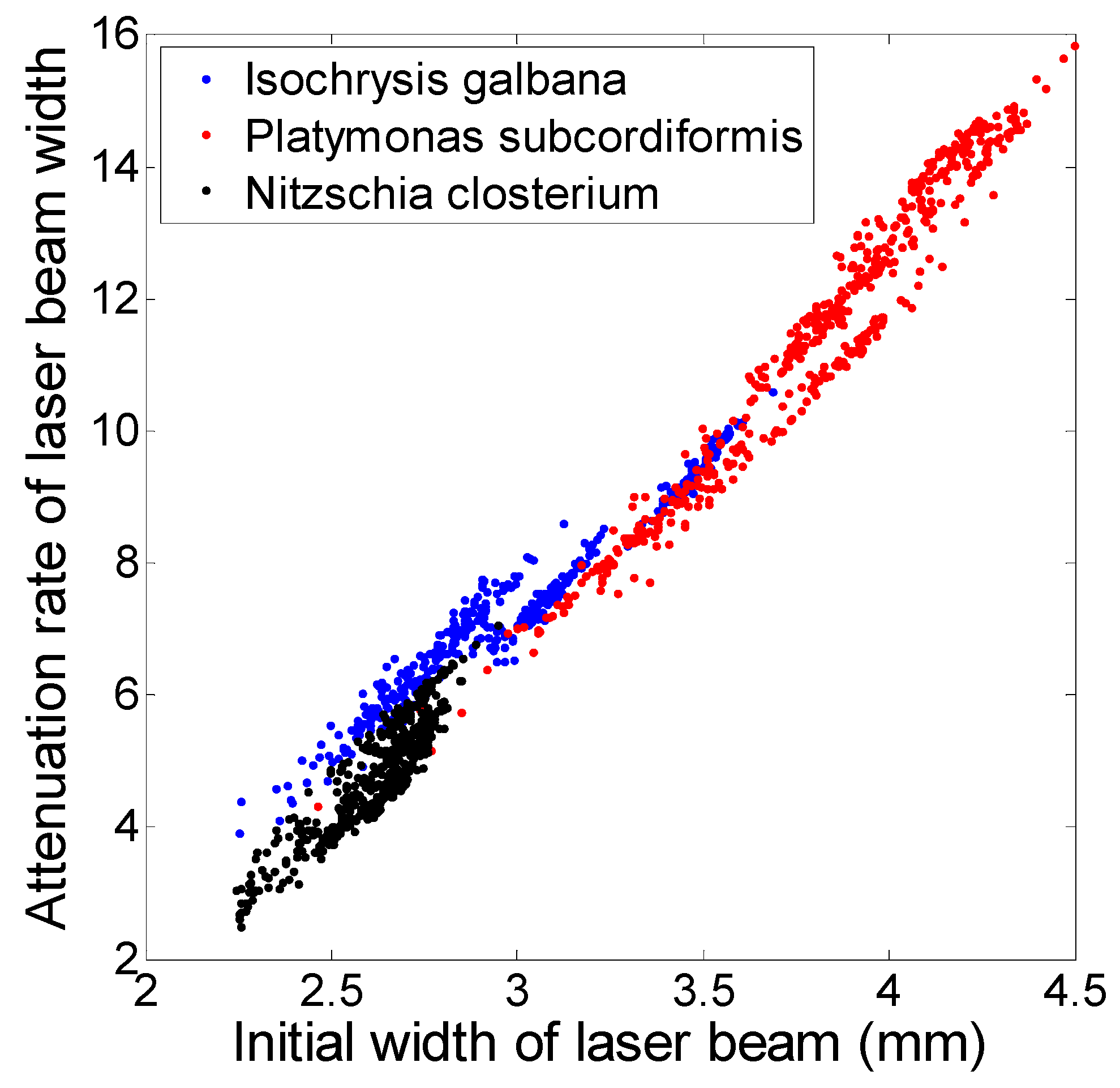
| Isochrysis galbana | Length: 4.4~7.1 Width: 2.7~4.4 Thickness: 2.4~3.0 |
| Platymonas subcordiformis | Length: 11.0~14.0 Width: 7.0~9.0 Thickness: 3.5~5.0 |
| Nitzschia closterium | Length: 12.0~23.0 Width: 2.0~3.0 Thickness: 2.4~3.0 |
| Water Types | a (m−1) | b (m−1) | c (m−1) |
|---|---|---|---|
| Pure sea water | 0.0405 | 0.0025 | 0.043 |
| Clear sea water | 0.114 | 0.037 | 0.151 |
| Coastal sea water | 0.179 | 0.219 | 0.398 |
| Turbid sea water | 0.366 | 1.824 | 2.190 |
Publisher’s Note: MDPI stays neutral with regard to jurisdictional claims in published maps and institutional affiliations. |
© 2021 by the authors. Licensee MDPI, Basel, Switzerland. This article is an open access article distributed under the terms and conditions of the Creative Commons Attribution (CC BY) license (https://creativecommons.org/licenses/by/4.0/).
Share and Cite
Zhang, H.; Zhang, Y.; Li, Z.; Liu, B.; Yin, B.; Wu, S. Small Angle Scattering Intensity Measurement by an Improved Ocean Scheimpflug Lidar System. Remote Sens. 2021, 13, 2390. https://doi.org/10.3390/rs13122390
Zhang H, Zhang Y, Li Z, Liu B, Yin B, Wu S. Small Angle Scattering Intensity Measurement by an Improved Ocean Scheimpflug Lidar System. Remote Sensing. 2021; 13(12):2390. https://doi.org/10.3390/rs13122390
Chicago/Turabian StyleZhang, Hongwei, Yuanshuai Zhang, Ziwang Li, Bingyi Liu, Bin Yin, and Songhua Wu. 2021. "Small Angle Scattering Intensity Measurement by an Improved Ocean Scheimpflug Lidar System" Remote Sensing 13, no. 12: 2390. https://doi.org/10.3390/rs13122390
APA StyleZhang, H., Zhang, Y., Li, Z., Liu, B., Yin, B., & Wu, S. (2021). Small Angle Scattering Intensity Measurement by an Improved Ocean Scheimpflug Lidar System. Remote Sensing, 13(12), 2390. https://doi.org/10.3390/rs13122390