Abstract
Land cover maps obtained at high spatial and temporal resolutions are necessary to support monitoring and management applications in areas with many smallholder and low-input agricultural systems, as those characteristic in Mozambique. Various regional and global land cover products based on Earth Observation data have been developed and made publicly available but their application in regions characterized by a large variety of agro-systems with a dynamic nature is limited by several constraints. Challenges in the classification of spatially heterogeneous landscapes, as in Mozambique, include the definition of the adequate spatial resolution and data input combinations for accurately mapping land cover. Therefore, several combinations of variables were tested for their suitability as input for random forest ensemble classifier aimed at mapping the spatial dynamics of smallholder agricultural landscape in Vilankulo district in Mozambique. The variables comprised spectral bands from Landsat 7 ETM+ and Landsat 8 OLI/TIRS, vegetation indices and textural features and the classification was performed within the Google Earth Engine cloud computing for the years 2012, 2015, and 2018. The study of three different years aimed at evaluating the temporal dynamics of the landscape, typically characterized by high shifting nature. For the three years, the best performing variables included three selected spectral bands and textural features extracted using a window size of 25. The classification overall accuracy was 0.94 for the year 2012, 0.98 for 2015, and 0.89 for 2018, suggesting that the produced maps are reliable. In addition, the areal statistics of the class classified as agriculture were very similar to the ground truth data as reported by the Serviços Distritais de Actividades Económicas (SDAE), with an average percentage deviation below 10%. When comparing the three years studied, the natural vegetation classes are the predominant covers while the agriculture is the most important cause of land cover changes.
1. Introduction
Food security, sustainable agricultural production, and poverty reduction are top priorities and challenging societal issues in Mozambique. The production and productivity of the main crops is very low due to limited use of improved agricultural inputs and the post-harvest losses are high. Therefore, the access to food for the gross part of Mozambican population relying on agricultural production is only guaranteed during short periods. As such, about 24% of households are food insecure and there is an extremely high level of chronic under-nutrition (43%) which affects almost one in every two children under the age of five years [1].
Mapping the cropland extent, distribution, and characteristics is of great importance to support measures to mitigate these priority problems in Mozambique. In fact, accurate and consistent information on cropland and the dynamic location of major crop types is required to support future policy, investment, and logistical decisions [2,3], as well as production monitoring [4]. Timely cropland information directly feeds early warning systems, such as FAO Global Information and Early Warning System (GIEWS), Global Monitoring for Food Security (GMFS), and Famine Early Warning Systems Network (FEWS NET) [5,6]. Moreover, this information is also relevant for other disciplines, such as environmental impact and mitigation measures of the foreseen climate scenarios [7]. In agriculture monitoring, as well as climate modeling, cropland maps can be used as a mask to isolate agricultural land for (1) time-series analysis for crop condition monitoring and (2) to examine how the cropland responds to different climatic scenarios [3]. Additionally, timely and accurate assessment of land cover and land use is essential in understanding how climate variability affects regional crop production and for supporting the allocation of resources for medium and long-term planning. This issue is particularly relevant considering that Mozambique is highly vulnerable to extreme weather events like droughts and floods (ranks 3rd amongst African countries) and to erratic and unpredictable precipitation patterns. These conditions contribute to instability in crop production and often limit access to food. Traditional smallholder and resources-poor farming systems dominate the agricultural landscape in Mozambique, with 99% of fields smaller than 1.5 hectares and growing mainly maize (Zea mays L.) or cassava (Manihot esculenta Crantz) for own consumption [8]. These traditional farming systems are characterized by a highly dynamic shifting nature because when the production starts to decline (in a time frame of very few years), the crop fields are left for fallow and new natural areas are open for cultivation.
Smallholder farmers constitute the socio-economic backbone of the country and provide the basis for food security, preserving natural biodiversity, and providing environmental protection [5]. It is therefore imperative to adopt data and tools that enable appropriate monitoring and mapping of these traditional agricultural systems so that they can be included and valued into more global food systems. On the other hand, to meet the rapidly growing demand for food, fueled by a rapid population growth and changing diets, and to enhance economic development, pressure on natural areas (forest and savannahs) is increasing [9,10]. Cultivating more land to increase yield has put natural land and water resources under intense pressure [11,12]. The introduction of agricultural machinery, the use of irrigation systems and fertilizers are contributing to rapidly modify the land surface. Given the rate of agricultural area expansion, the shifting nature of the dominant agricultural system and considering Mozambique’s vulnerability to risks from droughts and floods, there is a need to significantly improve the information management system aiming to feed crop statistics as well as to monitor and support the sustainable use of soil, water, and other resources [1]. In such context, the timely, accurate, and cost-efficient mapping of these peculiar and evolving agricultural systems in Mozambique, at fine scales, is paramount.
Remote sensing, through Earth Observation (EO) imagery, has been critical for land cover classification thanks to its wide area and time-repeated coverage. Several global land cover products have been developed and made publicly available. Among others, the following products are the most widespread: (i) the Global Land Cover database for the year 2000 (GLC2000), a SPOT4-based map produced by the European Commission’s Joint Research Center (JRC), with a spatial resolution of about 1 km at the equator and larger at higher latitudes [13,14,15]; (ii) the Globcover, produced by the European Space Agency with ENVISAT-MERIS data, with a 300 m of spatial resolution [16]; (iii) the Moderate-resolution Imaging Spectroradiometer (MODIS) Collection 5 Land Cover Product, with 500 m of spatial resolution [17]; (iv) the Global Land Cover Characterization database (GLCC), resulting from a concerted effort between the U.S. Geological Survey (USGS), University of Nebraska Lincoln (UNL) and the JRC, which is based on the Advanced Very High Resolution Radiometer (AVHRR) and has a nominal spatial resolution of 1 km [18]; (v) the Global Food Security-support Analysis Data Product (GFSAD1000), with a nominal scale of 1 km [19]; (vi) the global Spatial Production Allocation Model (SPAM) dataset, which utilizes several datasets and ancillary information, with a spatial resolution of about 10 km at the equator [13]; (vii) the International Institute for Applied Systems Analysis-International Food Policy Research Institute (IIASA-IFPRI) cropland product, a cropland percentage hybrid map generated using some of the datasets mentioned above, with a spatial resolution of 1 km [2]; the National Geomatic Center of China (NGCC) 30 m global land cover (Globeland 30), based on Landsat and China Environmental Disaster Alleviation Satellite (HJ – 1) [20].
In almost all the above-mentioned products, the coarse spatial resolution hinders the careful assessment of cropland class, which is characterized by a large variety of agro-systems with a dynamic nature. This issue is more pronounced in regions with prevalence of traditional smallholder and resource-poor farming systems, such as in many African countries [3,13,21]. In addition, the authors of [3,12,22] argued that some of these datasets are often not reliable over croplands, as they show important disagreement with each other and with national statistics. Other important limitations of the current global land cover maps are the lack of temporal updates, the limited number of land cover classes, and the types of classes defined, which are of limited use in finer scale applications [13].
There is growing interest in mapping smallholder dominated landscapes [23,24,25,26,27,28,29,30,31]. In general, smallholder cropland mapping is hindered by characteristics such as small field size, heterogeneity in management practices, landscape fragmentation, and the widespread presence of trees within the fields [24,32]. These characteristics differ widely between countries, agro-ecological zones, socio-economic context, and even region or province, making difficult the definition of the kind of spatial resolution and data input combinations for accurately mapping smallholders, as discussed by [30,32,33]. As such, there are studies reporting accurate land cover classification results within smallholder dominated landscapes using high-resolution imagery [29], very high-resolution imagery [23], or a combination [27]. The classification input data and the features calculated from the data, e.g., textural features at different window sizes, also impact on the classification accuracy, e.g., [33,34,35,36,37]. The textural features represent the spatial variation in contiguous pixel values and thus provide a quantitative measure of spatial context. These texture features are extracted through the application of multiple functions to the image bands at different window sizes, and thus can result in a large volume of input data with potentially relevant information for the classification [37]. Although the use of different sets of features in land cover classification has been widely explored, e.g., [34,35,38], more efforts are needed towards assessing the best combination of features when classifying shifting smallholder agricultural landscapes typical in several African countries as in Mozambique. According to [32] the selection of appropriate imagery and input feature for shifting smallholder classification is probably a context-specific issue.
The development of powerful cloud-based computational frameworks, coupled with the increasing accessibility of imagery resulting from the Landsat Global Archive Consolidation (LGAC) initiative [39] and the European Commission Copernicus programme (Sentinel 2A and 2B) [40] is making custom classification more accessible, and have the potential to help overcome the limitations of existing products. An example of the combined use of these assets is the Google Earth Engine (GEE), a planetary-scale platform for geospatial data science powered by Google’s cloud platform [41]. As pointed out by [13], GEE is an invaluable tool by making available a huge data pool of satellite imagery and access to robust algorithms that can be applied for diversified types of uses, including image classification. In fact, numerous studies have been developed to perform classification within GEE at regional [42,43,44,45] and global scales [46,47]. Amongst others, the frequently used classifiers include random forest (RF) [48]; support vector machine (SVM) [49], maximum entropy model (MaxEnt) [50]; classification and regression trees (CART) [51]. The RF, which is a classifier based on an ensemble of classification trees, has been demonstrated to provide higher accuracies in image classification applications than other techniques [52,53], independent of the type of data used and of the targeted environment. Moreover, RF is recognized by its ability to cope with a large set of input variables, which results from the use of a random subset of input features in the division of every node [37].
As highlighted by [54], the rising availability of improved RS data and tools offers the opportunity for the development of land cover and land uses maps at finer spatial and temporal resolutions, which are suitable to support applications in an agricultural setting with predominance of smallholder and resource-poor agricultural systems. This is particularly crucial in the face of rising climate variability and the associated uncertainties on smallholder agriculture [40]. Additionally, according to [3], Mozambique is one of the three Southern African countries of high priority for cropland mapping and which would really benefit from a timely land cover/land use update.
Most previous studies on smallholder cropland mapping considered only a single date or a single season time scale. However, making use of multitemporal imagery (from various years) is needed to capture both the spatial dynamics and the temporal shifting characteristic of smallholder agriculture in Mozambique.
In this context, the main objective of the current study is to develop and test an automated land cover classification and mapping for Vilankulo district in Mozambique using GEE cloud computing and based on different types of features derived from Landsat imagery for three years within the period between 2012 and 2018. The types of features tested include Landsat spectral bands, spectral vegetation indices, and textural features derived from the spectral bands. The specific objectives include (i) evaluating the best combination of input variables for the classification process; (ii) assessing the most adequate window size for the texture input features; (iii) assessing the spatial and temporal dynamics of agriculture in Vilankulo; (iv) comparing the statistics of agricultural areas as extracted from the produced maps to those yearly reported by the Local Government entities.
2. Materials and Methods
2.1. Study Area Description
The current study was conducted in the district of Vilankulo, within the province of Inhambane in southern Mozambique (Figure 1), and includes agricultural seasons of the years 2012, 2015, and 2018.
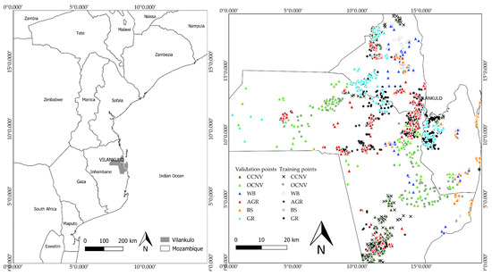
Figure 1.
Location of Vilankulo district in Mozambique (left) and map of Vilankulo district (right) with location of the training and validation datasets. CCNV—close canopy natural vegetation; OCNV—open canopy natural vegetation; WB—water bodies; AGR—agriculture; BS—bare soils; GR—grassland.
Climatologically, Vilankulo is characterized by a semi-arid to arid climate and presents two distinct seasons, a warm and rainy season running from October to March and a cold and dry season that runs from April to August.
The district of Vilankulo shapes well the complexity and heterogeneity of a landscape characterized by diversified land covers types, including agriculture, open and close canopy natural vegetation, water bodies, grasslands, bare soils, and human settlement areas. The agriculture is characterized by two cropping seasons, one during the rainy season and another during the dry season. The agriculture is mainly rainfed and is practiced only in the rainy season in mixed crop systems (maize, peanuts, beans, cassava, etc.); generally multipurpose trees species are also left within the crop fields for shade, fruits, medicines, and firewood collection. During the dry season, the rainfed croplands are not cultivated. In addition, rainfed croplands may be left for fallow after three or four years of consecutive cropping seasons, when the crop production drops considerably, and new natural areas are open for cultivation. Large scale irrigated crops (mainly maize, beans, soybean, and potatoes) have been introduced more recently and although grown throughout the entire year, it is still restricted to a small number of zones within the study area. Additionally, during the dry season, the cultivation is concentrated in areas neighboring water bodies (lagoons and rivers), where vegetables (e.g., tomatoes, cabbage, onion) are grown in small areas using handheld watering cans or small scales pumping irrigation systems.
The open-canopy natural vegetation (OCNV) comprises areas with vegetation bellow 5 m height and canopy cover below 10%; close canopy vegetation (CCNV) corresponds to areas with vegetation above 5 m height and canopy cover above or equal to 10%; water bodies (WB) comprise areas periodically or permanently covered by water; grasslands areas (GR) are primarily covered by grass with or without scattered shrubs; bare soils (BS) are uncovered areas which in the study area include prepared areas for agriculture, sand bands along water bodies; and agriculture (AGR) consists of cultivated fields.
2.2. Landsat Image Selection and Pre-Processing
Due to its high number of bands, Landsat 8 OLI/TIRS was taken as the prime source of data for the study and a search for all USGS Surface Reflectance (SR) images from the Landsat 8 OLI/TIRS sensor covering Vilankulo district in the main cropping seasons of 2015 and 2018 (October to March) was performed within the GEE’s data pool. The images used for each year are listed in Table 1.

Table 1.
Landsat 8 OLI/TIRS used in this study.
The study area is covered by three Landsat scenes of the path/row 166/75, 166/76, and 167/75.
Pre-processing of Landsat 8 OLI/TIRS images consisted of application of quality bands to remove cloud contamination.
For the year 2012, prior to the Landsat 8 OLI/TIRS launch (February 2013), a search for Landsat 7 ETM+ was done and six atmospherically corrected surface reflectance images and with cloud cover below 5% were identified. In this year, there was an anticipation of cropping season, taking advantage of good meteorological conditions observed in September. As such, an image of September was used for the scene with path/row 167/75. The USGS Gap-Fill algorithm, as implemented within GEE, was applied to fill the SLC-failure gaps in all selected Landsat 7 ETM+ images. The methodology involves using data from other scenes of the same reference (source scenes), to fill the gaps in the scenes of interest (fill scenes). The source scenes were selected within a time interval of less than four months relative to the date of the fill scenes (Table 2).
Table 2.
Landsat 7 ETM+ imagery used in the study.
2.3. Texture Features
Texture is a distinctive property of all surfaces. It contains important information about the spatial distribution, structural arrangement of surfaces, and their relationship to the surrounding environment [55]. Various methods can be used to derive textural information, for example, the first and second-order local statistics [56] and grey level co-occurrence matrix (GLCM) measurements [55]. Local statistics (LS) describe the moments of a neighborhood of individual pixels in an image region, while GLCM-based texture features characterize the distance and angular relationships among pixels. The GLCM is a tabulation of how often different combinations of pixel brightness values (grey levels) occur in an image. It counts the number of times a pixel of value X lies next to a pixel of value Y, in a given direction and distance, and then derives statistics from this tabulation. GLCM can be classified into two groups: (i) occurrence or first order measures, which describe a statistical property, such as pixel variance or skewness within a specified neighborhood of an image [57,58]; and (ii) co-occurrence or second order measures, which characterize the relative frequencies between two pixel brightness values linked by a spatial relation [59,60]. The second order GLCM texture measures have been the most common textural features used in remote sensing studies, including for forest structure modelling [61,62,63], habitat modelling [64], and land cover classification [65,66,67].
In this study, the 14 GLCM metrics proposed by [55], namely Angular Second Moment (asm), Contrast (contrast), Correlation (corr), Variance (var), Inverse Difference Moment (idm), Sum Average (savg), Sum Variance (svar), Sum Entropy (sent), Entropy (ent), Difference variance (dvar), Difference entropy (dent), Information Measure of correlation 1 (imcorr1), Information Measure of correlation 2 (imcorr2), and maximum correlation coefficient (maxcorr), and an additional four textural features from [68], specifically, Dissimilarity (diss), Inertia (inertia), Cluster Shade (shade) and Cluster prominence (prom), were computed for each Landsat band. As the value of texture variables depends mostly on window size and spatial resolution [61], six different window sizes (2, 5, 10, 20, 25, and 30) were tested while the 3 × 3 square default kernel size was kept constant.
2.4. Vegetation Indices
Four vegetation indices frequently used in land cover and agricultural studies were computed: normalized difference vegetation index (NDVI) [69]; soil adjusted vegetation index (SAVI) [70]; enhanced vegetation index (EVI) [71]; and the normalized water difference index (NWDI) [72]. NDVI is one of the most used vegetation indices for vegetation phenology characterization thanks to its sensitivity to photosynthetically active biomass and its ability to discriminate vegetation/non-vegetation, as well as wetland/non-wetland cover classes. SAVI was included to make use of its ability to minimize the soil background effect, as the study area presents large areas of sparse vegetation. EVI can be useful in areas of high leaf area index (LAI) where NDVI may saturate and NDWI is useful to discriminate water from land due to its sensitiveness to open water [73].
2.5. Image Composites
For each year studied, when more than one image per scene existed, an aggregation method on a per-pixel, per-band basis was applied by using the median value. The Pearson’s correlation coefficient was used to assess the correlation between Landsat bands. Bands of the same spectral region showed correlation coefficient greater than 0.90 for both visible and short-wave infrared regions. As such, only three bands were selected for further analysis, being the band 1, B1 (presenting the least correlation coefficient (0.24) with the B5); band 5, B5 (presenting the least correlation coefficient with all bands (0.36) in average); and band 6, B6 (presenting the least correlation with all bands (0.60), as compared to the B7, of the same spectral region).
The final image composites for the years 2015 and 2018 comprised 61 features: (i) three reflective Landsat 8 bands (Band 1—deep blue; Band 5—NIR; Band 6—SWIR1), (ii) four vegetation indices (NDVI, SAVI, EVI, and NWDI), and (iii) 54 GLCM textural features (18 GLCM × 3 bands). For the year 2012, the final image composites included the same numbers of features, but the textural features were extracted from reflective Landsat 7 bands (Band 1—blue; Band 4—NIR; Band 5—SWIR1).
2.6. Training and Validation Samples Collection
Six land cover types, characteristic of the study area landscape, were considered for image classification: (i) Close canopy natural vegetation (CCNV), (ii) Open canopy natural vegetation (OCNV), (iii) Water Bodies (WB), (iv) Agriculture, (v) Bare soils (BS), and Grassland (GR). Each land cover type is characterized according to the description provided in Section 2.1. The urban settlements were excluded from the classification process by using a mask derived from available cartography.
Global positioning system (GPS) points of each land cover type were collected during two field campaigns in 2017 and in 2019 and used as references during the on-screen collection of training data. During the field campaigns, farmers were asked about cultivation in previous years in order to ensure that only croplands operating for at least two consecutive years were included. The GPS points were then overlaid to the Landsat RGB and to very high-resolution Google Earth imagery of the corresponding cropping season and used as reference to select additional training samples. For the years where no ground data were available, the training data was selected based on visual inspection and interpretation of both Google Earth very high-resolution imagery and Landsat RGB composite. Visual interpretation of reference imagery was based on elements that help to identify land cover features such as location, size, shape, tone, color, shadow, texture, and pattern. A similar procedure was used by [74,75].
The validation data were generated by a stratified random sampling method from the classification results. The method was performed for each map (2012, 2015, and 2018) and, for each cover class, setting the number of validation points to at least 30% of the respective training points. This procedure enabled independence between training and validation data. It was also implemented in previous studies by [34]. Table 3 presents the number of training and validation samples used in each year and Figure 1 shows the spatial distribution of training and validation samples within the study area.
Table 3.
Number of training and validation samples per class and per year. CCNV—close canopy natural vegetation; OCNV—open canopy natural vegetation; WB—water bodies; AGR—agriculture; BS—bare soils; GR—grassland.
2.7. Input Features Selection for Classification
For the selection of optimal input features, the three non-correlated Landsat spectral bands, four vegetation indices (VIs), and the 18 GLCM textural features extracted in the three Landsat bands were initially considered.
Subsequently, combinations involving one or more types of the above features were established, including (Table 4) (i) Landsat bands and 18 GLCM per Landsat band (T1: Angular Second Moment (asm), Contrast (contrast), Correlation (corr), Variance (var), Inverse Difference Moment (idm), Sum Average (savg), Sum Variance (svar), Sum Entropy (sent), Entropy (ent), Difference variance (dvar), Difference entropy (dent), Information Measure of correlation 1 (imcorr1), Information Measure of correlation 2 (imcorr2), Maximum Correlation Coefficient (maxcorr), Dissimilarity (diss), Inertia (inertia), Cluster Shade (shade), Cluster prominence (prom)); (ii) Landsat bands and five GLCM textural features (T2: contrast, corr, variance, sevg, diss); (iii) Landsat bands and five GLCM textural features (T3: asm, shade, ent, prom, inertia); (iv) Landsat bands and six GLCM textural features (T4: asm, contrast, var, corr, ent, and idm); (v) Landsat bands; (vi) Landsat bands and four VIs.
Table 4.
Feature combinations as tested and average separability per class of land cover type, per feature combination, and average separability per feature combination.
For the combinations involving textural features, six different window sizes (2, 5, 10, 20, 25, and 30) were considered.
The subsets of five and six GLCM textural features selected for the combinations tested (#: 7–20 in Table 4) were identified among the most relevant according to the literature (asm, contrast, variance, correlation, entropy, inverse difference moment, dissimilarity) [60,76,77,78,79]. The textural features proposed by [68], were also included. These are suggested to improve the perceptual concepts of uniformity, proximity, and the qualities of texture periodicity and gradient, when combined with the so called most relevant GLCM textural metrics. The inverse divergence moment (idm) indicates the image homogeneity as it assumes larger values for smaller grey tone differences in pair elements. Contrast is a degree of spatial frequency, the difference between the maximum and the minimum values of a neighboring set of pixels; high contrast values denote high coarse texture. The dissimilarity (diss) informs about the heterogeneity of the grey levels; coarser textures present higher values of dissimilarity. Entropy (ent) indicates the disorder of an image; non-texturally uniform image presents very large entropy. Angular second moment (asm) is a measure of textural uniformity (pixel pair repetition); high asm values occur when the grey level distribution has either a contrast or a periodic form. Correlation (corr) indicates the grey tone linear dependencies in the image; high correlation values imply a linear relationship between the grey levels of pixel pairs. More information about the GLCM features can be found in [55,78].
The Jeffreys–Matusita distance (JM) was computed for each feature combination and all possible pair of classes. The JM is a pair-wise measure of class separability based on the probability distribution of two classes [80,81,82]. JM ranges from 0 to 2.0; values below 1.0 indicate that two classes are not separable; values between 1.0 and 1.5 indicate that two classes are separable but with some degree of confusion, and between 1.5 and 1.9, the classes are clearly separable; completely separable classes present JM values above 1.9 [38]. The selection of final feature combination considered the largest JM for the least separable pairs of classes, the number of features in the combination, and the GLCM window size. A similar approach was applied in previous studies [38,83,84].
2.8. Classifier Algorithm
In this study we used the random forest classifier (RF) [48], within the GEE platform. The RF can be described as the collection of tree-structured classifiers. It produces multiple decision trees, using randomly selected subsets of training samples and variables. As such, a classification result is obtained in each tree trained on a subset of the original training sample; subsequently a majority vote is used to create the final classification result. This classifier algorithm is considered very fast, robust against over fitting, allows forming as many trees as the user wants, and each decision tree uses a random subset of training data and a random subset of input predictor variables, which reduces the correlation between decision trees as well as the overall computational complexity [85]. In our study, a RF with 500 trees was created and the number of features per split was set to the square root of the total number of features, which corresponds to the standard settings [86].
2.9. Accuracy Assessment
A confusion matrix and the accuracy assessment of each map were computed using the validation data set for each land cover type. The widely applied overall accuracy (OA), Kappa coefficient (KC), producer accuracy (PA), and consumer accuracy (CA) were computed and used to assess the quality of derived land cover maps. The OA determines the overall efficiency of the algorithm and is measured by dividing the total number of correctly classified samples by the total number of the testing samples. The KC indicates the degree of agreement between the ground truth data and the predicted values. The PA measures how well a pixel has been classified. It includes the error of omission which refers to the proportion of observed features on the ground that are erroneously excluded from a class. The CA measures the reliability of the map, informing how well the map represents what is really on the ground and it includes the error of commission which refers to pixels erroneously included in a class [73,87].
Furthermore, the statistics of cropped areas for each year were computed and compared to those from the Local Government entity responsible for agricultural issues within the district (Serviços Distritais de Actividades Económicas, SDAE). SDAE estimates the agricultural area (ha) and production (ton) within the district based on the share of economically active population as reported by the National Census and share of population in agricultural sector, and the number and size of croplands as reported by the National Agrarian Census.
3. Results
3.1. Input Feature Selection
The separability analysis, based on the JM distance, shows that in 12 feature combinations tested (#: 1, 7, and 13–26), the average separability for all classes is bellow one, denoting that most of the classes are not separable. In the remaining features combinations (#: 2–6 and 8–12) the average separability is between 1 and 1.5 indicating that most of classes are separable but with some level of confusion (Table 4).
Except for the class CCNV, the other classes showed high sensitivity to the window size of textural features (Table 4), increasing the separability with the increase of the window size for the combinations #1–#12. For the combinations #13–#24, the pattern of separability between classes according to the window size was less evident.
The feature combinations #4 and #11 (Table 4) yielded very similar average separability for all classes and for these combinations more homogeneous separability results among classes were obtained (Table 5: #4–#11).
Table 5.
Jeffreys–Matusita distance for all possible pairs of classes as assessed for different feature combinations.
Considering the results presented in Table 4 and Table 5, combination #11 was selected for the classification in this study, taking over combination #4 mainly due to its relatively low number of features (18). The features in this combination include three Landsat bands and five GLCM textural measures (asm, shade, ent, prom, inertia) extracted from the three Landsat bands using window 25. For this feature combination, the least separable classes were grassland (GR) and open canopy natural vegetation (OCNV) and close canopy natural vegetation (CCNV) and agriculture (AGR). The highest separability was achieved between the following pairs of classes: GR and CCNV water bodies (WB); GR and; GR and agriculture (AGR); GR and bare soils (BS); OCNV and AGR and OCNV and WB (Table 5: #11).
3.2. Spatial and Temporal Dynamics of Agriculture
3.2.1. Classification Results
The spatial and temporal (2012, 2015, and 2018) distribution of each land cover class is mapped in Figure 2. Visual inspection of maps denotes increase of class agriculture (AGR) throughout the study period. Spatially, the cultivated area tends to span from north to the south of district while the western portion is predominately occupied by the class open canopy natural vegetation (OCNV), which is the most predominant class within all the study area.
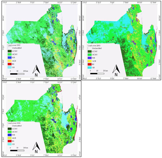
Figure 2.
Land cover maps of Vilankulo for the years 2012 (upper left), 2015 (upper right), and 2018 (lower left). CCNV—close canopy natural vegetation; OCNV—open canopy natural vegetation; WB—water bodies; AGR—agriculture; BS—bare soils; GR—grassland.
Table 6 presents the confusion matrices derived from the analysis of the validation dataset for each year. For the three years under consideration, the least accurately classified land cover class was OCNV. Most of OCNV incorrectly classified pixels were attributed to the classes CCNV, AGR, and GR. The class WB was consistently the most accurately classified with all the validation pixels correctly classified.
Table 6.
Confusion matrix of classification for the years 2012, 2015, and 2018. CCNV—close canopy natural vegetation; OCNV—open canopy natural vegetation; WB—water bodies; AGR—agriculture; BS—bare soils; GR—grassland; PA—producer accuracy; CA—consumer accuracy.
The classification overall accuracy (OA) and the kappa coefficient (KC) are presented in Table 7 for the three years. In all years both OA and KC present values consistently above 0.85, suggesting that all the classes were mapped with high accuracy.
Table 7.
Overall accuracy and Kappa coefficient.
3.2.2. Land Cover Statistics and Land Cover Changes
Table 8 and Table 9 present the land cover changes statistics, respectively, from 2012 to 2015 and from 2015 to 2018, as extracted from classification maps. The results indicate that the landscape of the study area is mostly occupied by natural vegetation classes, namely, close canopy natural vegetation (CCNV), open canopy natural vegetation (OCNV), and grassland (GR). Together the three classes comprise 86%, 85%, and 82% for the years 2012, 2015, and 2018, respectively. During the two time intervals, the changes in these classes occurred mainly within them but also between each of them and the class agriculture. The class agriculture (AGR) showed an increase from 68,417.28 ha in 2012 to 75,564.90 ha in 2015 and 89,442.72 ha in 2018. The water bodies remained almost unchanged from 2012 to 2015 but a larger increase was verified in the time interval between 2015 and 2018. The class bare soils (BS) experienced very small changes throughout the analyzed period (Table 8 and Table 9).
Table 8.
Land cover change matrix relative to the period 2012–2015.
Table 9.
Land cover change matrix relative to the period 2015–2018. CCNV—close canopy natural vegetation; OCNV—open canopy natural vegetation; WB—water bodies; AGR—agriculture; BS—bare soils; GR—grassland.
3.3. Comparison between Remote Sensed Classification and Agricultural Statistics
Due to data availability constraints, the comparison between remote sensing derived areas and ground truth data from statistical census was performed only for the class agriculture (AGR), for which annual statistical information is made available by a local Governmental Entity, the ‘Serviços Distritais de Actividades Económicas (SDAE)’. Figure 3 depicts the comparison between cultivated area as derived from the Landsat-derived maps and the SDAE data, denoting a good agreement between the two data sources. For the three studied years the mean percentage differences between actual ground truth data and remote sensed agrarian areas were below 10% and always negative, the highest deviation of 15.5% being observed in 2012. These measures of accuracy are in relation to the agrarian census, which also has its own inaccuracies.
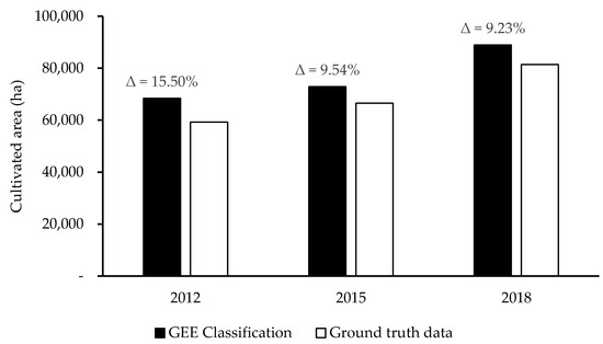
Figure 3.
Comparison between cultivated area derived from remote sensing data (classification results) and from ‘Serviços Distritais de Actividades Económicas (SDAE)’ (Local agrarian data). The percentage of overestimation of Google Earth Engine (GEE) classification relative to ground truth data is provided for each year.
4. Discussion
The selected input features for land cover classification in the study area include five GLCM textural features (angular second moment—asm, entropy—ent, inertia—inertia, cluster shade—shade, cluster prominence—prom), and three Landsat spectral bands (Band 1—deep blue, Band 5—NIR, and Band 6—SWIR1 for Landsat 8; and Band 1—blue, Band 4—NIR, and Band 5—SWIR1 for Landsat 7). Several studies have shown that integrating optical spectral data with texture features representing the spatial variability in pixel values can improve classification accuracy [33]. The textural features asm and ent have been included as optimal features for land cover classification in previous studies, e.g., [76,78,79]. In this study, asm and ent performed poorly when combined together with other so called most relevant textural features (texture features combinations #17–#20; Table 5), but results improved when asm and ent were combined with the textural features inertia, shade, and prom (texture features combinations #1–#12; Table 5). These results suggest that textural features inertia, shade, and prom may have improved the separability of different cover classes as argued by [68]. The Landsat spectral bands selected in this study are widely used as important features for land cover classification in diversified types of landscapes [13,88,89]. The increase of window values for textural feature extraction showed notable gain in land cover class separability up to window equal to 25 for combinations #1–#12 (Table 4). The increase of class separability with the increase of window is plausible for the study area which presents high degree of spatial variability. In a previous study, the authors [35] concluded that for areas displaying a lower degree of spatial variation small window sizes perform better, while for heterogeneous landscapes texture features extracted using large window values highly improve the classification accuracies. The fact that in this study the class close canopy natural vegetation (CCNV) was insensitive to window increase in several combinations of features may be explained by the within homogeneity that characterizes this type of land cover class in the study area.
Overall, the separability between the land cover classes was good. Lower separability occurred between open canopy natural vegetation (OCNV) and grassland (GR) and close canopy natural vegetation (CCNV) and agriculture (AGR) (Table 4 and Table 5). The low separability between OCNV and GR could be explained by the fact that the distinction of these classes was based on the tree/shrub cover percentage or density as observed in the field and from high-resolution imagery. Nevertheless, the two classes may present similar spectral behavior as consequence of defoliation of the trees comprising the upper canopy. Defoliation and leaf development have been indicated as the main factor of seasonality of spectral behavior in deciduous forest canopies [90,91]. When the defoliation occurs in the upper canopy trees, the spectral signature of the site is dominated by the understory vegetation. The opposite is verified in case of leaf development [90]. Other authors also reported lower separability performance between land cover classes related with sparse vegetation and low shrublands [88]. The low separability between CCNV and AGR may be explained by the fact that in the study area, forest areas are characterized by high fragmentation, with interstices occupied by other land cover types including AGR. Additionally, AGR is characterized by mixed crop systems, which generally include multipurpose trees within the fields. Additionally, in [92] the authors reported the complexity of classifying mosaic areas comprising different proportions of various homogeneous classes including forests.
The overall accuracy of the classification performed in this study (percentage values: 89%–98%; Table 7) outperformed the results of previous studies equally using the random forest algorithm with varying data types and in diversified types of landscapes and area extensions. For example, 85% overall accuracy in crop type classification using a multi-spectral time series of RapidEye images [93]; more than 80% for a time series of Landsat 7 images in homogeneous regions [94]; around 89% for a time series of Landsat 7 and 8 in heterogeneous regions [13]; up to 71.7 for Worldview 2 time series in heterogeneous regions [95] and 85.9% for crop discrimination using SPOT 5 images [96]. This may be attributed to the fact that in this study, a reduced spatial extent was under consideration, what made it easier to take the local conditions into account and tune the classification accordingly. Nevertheless, the overall accuracy of these studies reports to different land cover classes, including classes relative to different crop types. The lower classification accuracy for the year 2018 (0.89) as compared to the years 2012 (0.94) and 2015 (0.98) may equally be justified by the high fragmentation of forest areas within the study area. In fact, from Figure 2 it is noticeable that the forest fragmentation is higher in 2018, mainly due to agricultural expansion. Due to the early mentioned characteristics of agricultural systems, the confusion between this class and the forested areas is higher in 2018, what is confirmed in the confusion matrices presented in the Table 6.
Most OCNV misclassified pixels were erroneously classified as other vegetated classes (CCNV, AGR, and GR). This may be due to the seasonality in canopy spectral signature, which is characteristic in deciduous vegetation [90]. In fact, within the study area, CCNV pixels may temporally seem OCNV due to defoliation and the same process can make OCNV appear similar to AGR or GR. The inaccurately classified BS pixels as AGR (Table 6) could be due to the effect of soil background during initial stages of crop development, as various satellite images used in the classification were from dates corresponding to the initial phase of crops growth cycle (Table 1).
The land cover analysis showed that the study area landscape is predominantly covered by natural vegetation classes (CCNV, OCNV, and GR), and experiences a strong dynamic from one land cover class to another (Figure 2). Changes between the three natural vegetation classes appear to be largely due to spectral similarities caused by vegetation seasonality characteristics rather than due to conversion from one to another class. Similar findings were reported in previous studies, e.g., [35,38,78]. As was expected, the class agriculture (AGR) ranks first as the driving of effective land cover conversion, specifically for the class OCNV. During the period 2012–2018 a total of 60,945.12 ha of OCNV area was converted into AGR while 74,752.38 ha was recovered from AGR to OCNV. In the same period, a total of 16,203.78 ha was converted from all other cover classes to AGR (Table 8 and Table 9). These land cover dynamic of transitions from AGR to other classes and vice-versa confirms the shifting nature of agriculture in the study area, which is characterized by systematically leaving old croplands for fallow and setting new areas for cultivation in natural vegetation areas. As pointed out by [9,11,97], in most African countries natural areas (forests and savannas) are under increasing pressure as the cultivation of more and more land is the means to meet the growing food demand. Additionally, the authors of [11,97,98,99] pointed out that anthropogenic land conversion is a primary cause of habitat and biodiversity loss.
The statistics of agriculture area as derived from the classification are relatively greater than those reported by the Local Governmental Entity, the SDAE, but the mean difference for the three years is rather low (slightly above 10%; Figure 3). The SDAE’s statistics, as the overall agricultural statistics relying on farm surveys, have their own accuracy errors, which may result from the respondent (literacy degree, mistrust), the interviewer, the survey instrument (questionnaire design), the mode of data collection, and the incompleteness of the census list. The mean difference between the satellite-based classification and ground truth statistics from SDAE are within the average error of field surveys based agricultural censuses in developing countries (average error of 11% between the area measured and the area estimated by farmers) [99].
In a study to map cropping intensity of smallholder farms in India, the authors [25] reported a large discrepancy between cropped area estimated through remote sensing, using Landsat data, and the area of agricultural census (percentage difference of 150.8%). Likewise, [100] the authors found that irrigation area derived using MODIS 500 m data was consistently greater than the ground truth data in most of the Indian States but the percentage difference was of about 17.2%.
The good accuracy results obtained for the maps produced in this study indicate their reliability for cropland area estimation, while adding a spatially distribution information. This finding is very important considering that cropland mapping is a pre-requisite for crop monitoring through remote sensing.
The applied methodology may most likely be applied straightforward in other districts of Mozambique, given the similarities of agricultural systems. However, its application in other locations across the globe, should be considered with care as the appropriateness of a method depends on the goals of the study, the scale of analysis, and the characteristics of the agricultural system in question [30,32,33].
5. Conclusions
In this study, Google Earth Engine cloud computing was successfully applied for land cover classification in Vilankulo district in Mozambique. The best performing input variables for the random forest ensemble classifier were identified through systematic testing of different types of features. The selected input features included spectral bands and texture features. Furthermore, the best window size for the texture features computation was selected based on land cover classes separability, allowing the identification of the classes with higher sensitivity to this specific parameter in liaison to the inherent specificities of each class. The classification was applied to various years allowing to evaluate the shifting dynamics of smallholder agriculture in a time frame between 2012 and 2018.
The classes close canopy natural vegetation (CCNV), open canopy natural vegetation (OCNV), and grassland (GR) are the prevalent land cover types within the district while agriculture (AGR) is the most important cause of land cover change either by opening new cropping fields or by leaving the old ones for fallow. The cultivated area consistently increased throughout the entire study period and new spatial patterns were identified, with more concentrated agriculture areas spanning to the south east portion of the district.
The produced maps yielded high overall accuracy and the derived agricultural statistics present reasonable agreement with the ground truth statistics from SDAE.
The operational applications of this study results include timely and spatially distributed monitoring of agricultural areas, which can contribute to the improvement of agricultural statistics, to support local decisions regarding agriculture management and associated inputs management (e.g., irrigation water), to feed crop growth simulation models, among others. Additionally, the results allow the monitoring of natural vegetation dynamics for several years, which can support management decisions related to biodiversity and natural resources conservation. Moreover, on demand products may be derived based upon the methodology developed. Nevertheless, future research should address testing other types of remote sensing data (e.g., Sentinel-1 and Sentinel-2) either paired or not paired with Landsat data.
Author Contributions
Conceptualization, S.M., I.P. and M.C.; methodology, S.M., I.P. and M.C.; validation, I.P. and M.C.; formal analysis, S.M.; writing—original draft preparation, S.M.; supervision, I.P. and M.C. All authors have read and agreed to the published version of the manuscript.
Funding
This research received no external funding.
Acknowledgments
Sosdito Mananze acknowledges the Austrian Partnership Programme in Higher Education & Research for Development (APPEAR) for the funding through the project EO4Africa; the Ministério de Ciência e Tecnologia, Ensino Superior e Técnico Profissional, for the funding through the HEST project and Emma Izquierdo-Verdiguier for her support with the Google Earth code writing, and Isabel Pôças acknowledges the Post-Doctoral grant of the Research Infrastructure Enabling Green E-science for the SKA (ENGAGE-SKA) funded by COMPETE2020 and Fundação para a Ciência e a Tecnologia (POCI-01-0145-FEDER-022217).
Conflicts of Interest
The authors declare no conflict of interest.
References
- FAO. FAO, Country Programming Framework for Mozambique 2016–2020; FAO: Maputo, Mozambique, 2016; p. 13. [Google Scholar]
- Fritz, S.; See, L.; McCallum, I.; You, L.; Bun, A.; Moltchanova, E.; Duerauer, M.; Albrecht, F.; Schill, C.; Perger, C.; et al. Mapping global cropland and field size. Glob. Chang. Biol. 2015, 21, 1980–1992. [Google Scholar] [CrossRef]
- Waldner, F.; Fritz, S.; Di Gregorio, A.; Defourny, P. Mapping Priorities to Focus Cropland Mapping Activities: Fitness Assessment of Existing Global, Regional and National Cropland Maps. Remote Sens. 2015, 7, 7959–7986. [Google Scholar] [CrossRef]
- Justice, C.O.; Becker-Reshef, I. Report from the Workshop on Developing a Strategy for Global Agricultural Monitoring in the Framework of Group on Earth Observations (GEO); UN FAO: Rome, Italy, 2007; p. 67. [Google Scholar]
- Hannerz, F.; Lotsch, A. Assessment of remotely sensed and statistical inventories of African agricultural fields. Int. J. Remote Sens. 2008, 29, 3787–3804. [Google Scholar] [CrossRef]
- Vancutsem, C.; Marinho, E.; Kayitakire, F.; See, L.; Fritz, S. Harmonizing and combining existing land cover/land use datasets for cropland area monitoring at the African continental scale. Remote Sens. 2012, 5, 22. [Google Scholar] [CrossRef]
- Lobell, D.B.; Bala, G.; Duffy, P.B. Biogeophysical impacts of cropland management changes on climate. Geophys. Res. Lett. 2006, 33. [Google Scholar] [CrossRef]
- INE. Censo Agro-Pecuário CAP 2009–2010: Resultados preliminares-Moçambique; Instituto Nacional de Estatistcas: Madrid, Spain, 2011; p. 125. [Google Scholar]
- Morris, M.B.H.; Byerlee, D.; Savanti, P.; Staatz, J. Awakening Africa’s Sleeping Giant: Prospects for Commercial Agriculture in the Guinea Savannah Zone and Beyond; The World Bank: Washington, DC, USA, 2009. [Google Scholar]
- United Nations. World Population Prospects: The 2012 Revision, Highlights and Advance Tables; United Nations: New York, NY, USA, 2013. [Google Scholar]
- Brink, A.B.; Eva, H.D. Monitoring 25 years of land cover change dynamics in Africa: A sample based remote sensing approach. Appl. Geogr. 2009, 29, 12. [Google Scholar] [CrossRef]
- Ramankutty, N.; Evan, A.T.; Monfreda, C.; Foley, J.A. Farming the planet: 1. Geographic distribution of global agricultural lands in the year 2000. Glob. Biogeochem. Cycles 2008, 22. [Google Scholar] [CrossRef]
- Azzari, G.; Lobell, D.B. Landsat-based classification in the cloud: An opportunity for a paradigm shift in land cover monitoring. Remote Sens. Environ. 2017, 202, 64–74. [Google Scholar] [CrossRef]
- Bartholomé, E.; Belward, A.S. GLC2000: A new approach to global land cover mapping from Earth observation data. Int. J. Remote Sens. 2005, 26, 1959–1977. [Google Scholar] [CrossRef]
- Fritz, S.; Bartholomé, E.; Belward, A.; Hartley, A.; Stibig, H.J.; Eva, H.; Mayaux, P.; Bartalev, S.; Latifovic, R.; Kolmert, S.; et al. Harmonisation, Mosaicing and Production of the Global Land Cover 2000 Database (Beta Version); EC-JRC: Ispra, Italy, 2003. [Google Scholar]
- Arino, O.; Gross, D.; Ranera, F.; Leroy, M.; Bicheron, P.; Brockman, C.; Defourny, P.; Vancutsem, C.; Achard, F.; Durieux, L.; et al. GlobCover: ESA service for global land cover from MERIS. In Proceedings of the 2007 IEEE International Geoscience and Remote Sensing Symposium, Barcelona, Spain, 23–28 July 2007; pp. 2412–2415. [Google Scholar]
- Friedl, M.A.; Sulla-Menashe, D.; Tan, B.; Schneider, A.; Ramankutty, N.; Sibley, A.; Huang, X. MODIS Collection 5 global land cover: Algorithm refinements and characterization of new datasets. Remote Sens. Environ. 2010, 114, 168–182. [Google Scholar] [CrossRef]
- Loveland, T.R.; Reed, B.C.; Brown, J.F.; Ohlen, D.O.; Zhu, Z.; Yang, L.; Merchant, J.W. Development of a global land cover characteristics database and IGBP DISCover from 1 km AVHRR data. Int. J. Remote Sens. 2000, 21, 1303–1330. [Google Scholar] [CrossRef]
- Thenkabail, P.S.; Knox, J.W.; Ozdogan, M.; Gumma, M.K.; Congalton, R.G.; Wu, Z.; Milesi, C.; Finkral, A.; Marshall, M.; Mariotto, I.; et al. Assessing future risks to agricultural productivity, water resources and food security: How can remote sensing help? Photogramm. Eng. Remote Sens. 2012, 78, 773–782. [Google Scholar]
- Chen, J.; Chen, J.; Liao, A.; Cao, X.; Chen, L.; Chen, X.; He, C.; Han, G.; Peng, S.; Lu, M.; et al. Global land cover mapping at 30m resolution: A POK-based operational approach. ISPRS J. Photogramm. Remote Sens. 2015, 103, 7–27. [Google Scholar] [CrossRef]
- Anderson, W.; You, L.; Wood, S.; Wood-Sichra, U.; Wu, W. An analysis of methodological and spatial differences in global cropping systems models and maps. Glob. Ecol. Biogeogr. 2015, 24, 180–191. [Google Scholar] [CrossRef]
- Fritz, S.; See, L.; McCallum, I.; Schill, C.; Obersteiner, M.; van der Velde, M.; Boettcher, H.; Havlík, P.; Achard, F. Highlighting continued uncertainty in global land cover maps for the user community. Environ. Res. Lett. 2011, 6, 044005. [Google Scholar] [CrossRef]
- Debats, S.R.; Luo, D.; Estes, L.D.; Fuchs, T.J.; Caylor, K.K. A generalized computer vision approach to mapping crop fields in heterogeneous agricultural landscapes. Remote Sens. Environ. 2016, 179, 210–221. [Google Scholar] [CrossRef]
- Delrue, J.; Bydekerke, L.; Eerens, H.; Gilliams, S.; Piccard, I.; Swinnen, E. Crop mapping in countries with small-scale farming: A case study for West Shewa, Ethiopia. Int. J. Remote Sens. 2013, 34, 2566–2582. [Google Scholar] [CrossRef]
- Jain, M.; Mondal, P.; DeFries, R.S.; Small, C.; Galford, G.L. Mapping cropping intensity of smallholder farms: A comparison of methods using multiple sensors. Remote Sens. Environ. 2013, 134, 210–223. [Google Scholar] [CrossRef]
- Jin, Z.; Azzari, G.; You, C.; Di Tommaso, S.; Aston, S.; Burke, M.; Lobell, D.B. Smallholder maize area and yield mapping at national scales with Google Earth Engine. Remote Sens. Environ. 2019, 228, 115–128. [Google Scholar] [CrossRef]
- Lebourgeois, V.; Dupuy, S.; Vintrou, É.; Ameline, M.; Butler, S.; Bégué, A. A Combined Random Forest and OBIA Classification Scheme for Mapping Smallholder Agriculture at Different Nomenclature Levels Using Multisource Data (Simulated Sentinel-2 Time Series, VHRS and DEM). Remote Sens. 2017, 9, 259. [Google Scholar] [CrossRef]
- McCarty, J.L.; Neigh, C.S.R.; Carroll, M.L.; Wooten, M.R. Extracting smallholder cropped area in Tigray, Ethiopia with wall-to-wall sub-meter WorldView and moderate resolution Landsat 8 imagery. Remote Sens. Environ. 2017, 202, 142–151. [Google Scholar] [CrossRef]
- Sweeney, S.; Ruseva, T.; Estes, L.; Evans, T. Mapping Cropland in Smallholder-Dominated Savannas: Integrating Remote Sensing Techniques and Probabilistic Modeling. Remote Sens. 2015, 7, 15295–15317. [Google Scholar] [CrossRef]
- Timmermans, A. Mapping Cropland in Smallholder Farmer Systems in South-Africa Using Sentinel-2 Imagery; Université Catholique de Louvain: Louvain, Belgium, 2018. [Google Scholar]
- Vogels, M.; De Jong, S.; Sterk, G.; Douma, H.; Addink, E. Spatio-Temporal Patterns of Smallholder Irrigated Agriculture in the Horn of Africa Using GEOBIA and Sentinel-2 Imagery. Remote Sens. 2019, 11, 143. [Google Scholar] [CrossRef]
- Lambert, M.-J.; Pierre, T.; Xavier, B.; Philippe, B.; Pierre, D. Estimating smallholder crops production at village level from Sentinel-2 time series in Mali’s cotton belt. Remote Sens. Environ. 2018, 216. [Google Scholar] [CrossRef]
- Räsänen, A.; Virtanen, T. Data and resolution requirements in mapping vegetation in spatially heterogeneous landscapes. Remote Sens. Environ. 2019, 230, 111207. [Google Scholar] [CrossRef]
- Chen, W.; Li, X.; He, H.; Wang, L. Assessing Different Feature Sets’ Effects on Land Cover Classification in Complex Surface-Mined Landscapes by ZiYuan-3 Satellite Imagery. Remote Sensing 2018, 10, 23. [Google Scholar] [CrossRef]
- Coburn, C.A.; Roberts, A.C.B. A multiscale texture analysis procedure for improved forest stand classification. Int. J. Remote Sens. 2004, 25, 4287–4308. [Google Scholar] [CrossRef]
- Khatami, R.; Mountrakis, G.; Stehman, S.V. A meta-analysis of remote sensing research on supervised pixel-based land-cover image classification processes: General guidelines for practitioners and future research. Remote Sens. Environ. 2016, 177, 89–100. [Google Scholar] [CrossRef]
- Rodriguez-Galiano, V.F.; Chica-Olmo, M.; Abarca-Hernandez, F.; Atkinson, P.M.; Jeganathan, C. Random Forest classification of Mediterranean land cover using multi-seasonal imagery and multi-seasonal texture. Remote Sens. Environ. 2012, 121, 93–107. [Google Scholar] [CrossRef]
- Wu, W.; Zucca, C.; Karam, F.; Liu, G. Enhancing the performance of regional land cover mapping. Int. J. Appl. Earth Obs. Geoinf. 2016, 52, 422–432. [Google Scholar] [CrossRef]
- Wulder, M.A.; White, J.C.; Loveland, T.R.; Woodcock, C.E.; Belward, A.S.; Cohen, W.B.; Fosnight, E.A.; Shaw, J.; Masek, J.G.; Roy, D.P. The global Landsat archive: Status, consolidation, and direction. Remote Sens. Environ. 2016, 185, 271–283. [Google Scholar] [CrossRef]
- Kpienbaareh, D.; Kansanga, M.; Luginaah, I. Examining the potential of open source remote sensing for building effective decision support systems for precision agriculture in resource-poor settings. GeoJournal 2018. [Google Scholar] [CrossRef]
- Gorelick, N.; Hancher, M.; Dixon, M.; Ilyushchenko, S.; Thau, D.; Moore, R. Google Earth Engine: Planetary-scale geospatial analysis for everyone. Remote Sens. Environ. 2017, 202, 18–27. [Google Scholar] [CrossRef]
- Dong, J.; Xiao, X.; Menarguez, M.A.; Zhang, G.; Qin, Y.; Thau, D.; Biradar, C.; Moore, B. Mapping paddy rice planting area in northeastern Asia with Landsat 8 images, phenology-based algorithm and Google Earth Engine. Remote Sens. Environ. 2016, 185, 142–154. [Google Scholar] [CrossRef]
- Padarian, J.; Minasny, B.; McBratney, A.B. Using Google’s cloud-based platform for digital soil mapping. Comput. Geosci. 2015, 83, 80–88. [Google Scholar] [CrossRef]
- Patel, N.N.; Angiuli, E.; Gamba, P.; Gaughan, A.; Lisini, G.; Stevens, F.R.; Tatem, A.J.; Trianni, G. Multitemporal settlement and population mapping from Landsat using Google Earth Engine. Int. J. Appl. Earth Obs. Geoinf. 2015, 35, 199–208. [Google Scholar] [CrossRef]
- Simonetti, D.; Simonetti, E.; Szantoi, Z.; Lupi, A.; Eva, H.D. First Results from the Phenology-Based Synthesis Classifier Using Landsat 8 Imagery. IEEE Geosci. Remote Sens. Lett. 2015, 12, 1496–1500. [Google Scholar] [CrossRef]
- Hansen, M.C.; Potapov, P.V.; Moore, R.; Hancher, M.; Turubanova, S.A.; Tyukavina, A.; Thau, D.; Stehman, S.V.; Goetz, S.J.; Loveland, T.R.; et al. High-Resolution Global Maps of 21st-Century Forest Cover Change. Science 2013, 342, 850–853. [Google Scholar] [CrossRef]
- Pekel, J.-F.; Cottam, A.; Gorelick, N.; Belward, A.S. High-resolution mapping of global surface water and its long-term changes. Nature 2016, 540, 418. [Google Scholar] [CrossRef]
- Breiman, L. Random Forests. Mach. Learn. 2001, 45, 5–32. [Google Scholar] [CrossRef]
- Cortes, C.; Vapnik, V. Support-vector networks. Mach. Learn. 1995, 20, 273–297. [Google Scholar] [CrossRef]
- Phillips, S.J.; Anderson, R.P.; Schapire, R.E. Maximum entropy modeling of species geographic distributions. Ecol. Model. 2006, 190, 231–259. [Google Scholar] [CrossRef]
- Breiman, L.; Friedman, J.; Stone, C.; Olshen, R. Classification and Regression Trees; Chapman&Hall/CRC: Boca Raton, FL, USA, 1984. [Google Scholar]
- Belgiu, M.; Drăguţ, L. Random forest in remote sensing: A review of applications and future directions. ISPRS J. Photogramm. Remote Sens. 2016, 114, 24–31. [Google Scholar] [CrossRef]
- Gómez, C.; White, J.C.; Wulder, M.A. Optical remotely sensed time series data for land cover classification: A review. ISPRS J. Photogramm. Remote Sens. 2016, 116, 55–72. [Google Scholar] [CrossRef]
- Pretty, J.N.; Noble, A.D.; Bossio, D.; Dixon, J.; Hine, R.E.; Penning de Vries, F.W.T.; Morison, J.I.L. Resource-Conserving Agriculture Increases Yields in Developing Countries. Environ. Sci. Technol. 2006, 40, 1114–1119. [Google Scholar] [CrossRef] [PubMed]
- Haralick, R.M.; Shanmugam, K.; Dinstein, I. Textural Features for Image Classification. IEEE Trans. Syst. ManCybern. 1973, SMC-3, 610–621. [Google Scholar] [CrossRef]
- Kuplich, T.M.; Curran, P.J.; Atkinson, P.M. Relating SAR image texture to the biomass of regenerating tropical forests. Int. J. Remote Sens. 2005, 26, 4829–4854. [Google Scholar] [CrossRef]
- Asner, G.P.; Palace, M.; Keller, M.; Pereira, R., Jr.; Silva, J.N.M.; Zweede, J.C. Estimating Canopy Structure in an Amazon Forest from Laser Range Finder and IKONOS Satellite Observations1. Biotropica 2002, 34, 483–492. [Google Scholar] [CrossRef]
- Wright, C.; Gallant, A. Improved wetland remote sensing in Yellowstone National Park using classification trees to combine TM imagery and ancillary environmental data. Remote Sens. Environ. 2007, 107, 582–605. [Google Scholar] [CrossRef]
- Augusteijn, M.F.; Clemens, L.E.; Shaw, K.A. Performance evaluation of texture measures for ground cover identification in satellite images by means of a neural network classifier. IEEE Trans. Geosci. Remote Sens. 1995, 33, 616–626. [Google Scholar] [CrossRef]
- Baraldi, A.; Parmiggiani, F. An investigation of the textural characteristics associated with Gray Level Co-occurrence Matrix statistical parameters. Geosci. Remote Sens. IEEE Trans. 1995, 33, 293–304. [Google Scholar] [CrossRef]
- Castillo-Santiago, M.; Ricker, M.; Jong, B. Estimation of tropical forest structure from SPOT5 satellite images. Int. J. Remote Sens. 2010, 31, 2767–2782. [Google Scholar] [CrossRef]
- Kayitakire, F.; Hamel, C.; Defourny, P. Retrieving forest structure variables based on image texture analysis and IKONOS-2 imagery. Remote Sens. Environ. 2006, 102, 390–401. [Google Scholar] [CrossRef]
- Ozdemir, I.; Karnieli, A. Predicting forest structural parameters using the image texture derived from WorldView-2 multispectral imagery in a dryland forest, Israel. Int. J. Appl. Earth Obs. Geoinf. 2011, 13, 701–710. [Google Scholar] [CrossRef]
- Estes, L.D.; Reillo, P.R.; Mwangi, A.G.; Okin, G.S.; Shugart, H.H. Remote sensing of structural complexity indices for habitat and species distribution modeling. Remote Sens. Environ. 2010, 114, 792–804. [Google Scholar] [CrossRef]
- Beekhuizen, J.; Clarke, K.C. Toward accountable land use mapping: Using geocomputation to improve classification accuracy and reveal uncertainty. Int. J. Appl. Earth Obs. Geoinf. 2010, 12, 127–137. [Google Scholar] [CrossRef]
- Kimothi, M.; Dasari, A. Methodology to map the spread of an invasive plant (Lantana camara L.) in forest ecosystems using Indian remote sensing satellite data. Int. J. Remote Sens. 2010, 31, 3273–3289. [Google Scholar] [CrossRef]
- Pacifici, F.; Chini, M.; Emery, W.J. A neural network approach using multi-scale textural metrics from very high-resolution panchromatic imagery for urban land-use classification. Remote Sens. Environ. 2009, 113, 1276–1292. [Google Scholar] [CrossRef]
- Conners, R.W.; Trivedi, M.M.; Harlow, C.A. Segmentation of a high-resolution urban scene using texture operators. Comput. Vis. Graph. Image Process. 1984, 25, 273–310. [Google Scholar] [CrossRef]
- Rouse, J.W.; Haas, R.H.; Schell, J.A.; Deering, D.W. Monitoring vegetation systems in the Great Plains with ERTS. Proceedings of Third Earth Resources Technology Satellite Symposium, Washington, DC, USA, 10–14 December 1973; p. 9. [Google Scholar]
- Huete, A.R. A soil-adjusted vegetation index (SAVI). Remote Sens. Environ. 1988, 25, 295–309. [Google Scholar] [CrossRef]
- Huete, A.; Didan, K.; Miura, T.; Rodriguez, E.P.; Gao, X.; Ferreira, L.G. Overview of the radiometric and biophysical performance of the MODIS vegetation indices. Remote Sens. Environ. 2002, 83, 195–213. [Google Scholar] [CrossRef]
- McFeeters, S.K. The use of the Normalized Difference Water Index (NDWI) in the delineation of open water features. Int. J. Remote Sens. 1996, 17, 1425–1432. [Google Scholar] [CrossRef]
- Mahdianpari, M.; Salehi, B.; Mohammadimanesh, F.; Homayouni, S.; Gill, E. The First Wetland Inventory Map of Newfoundland at a Spatial Resolution of 10 m Using Sentinel-1 and Sentinel-2 Data on the Google Earth Engine Cloud Computing Platform. Remote Sens. 2018, 11, 43. [Google Scholar] [CrossRef]
- De Alban, J.D.; Connette, G.; Oswald, P.; Webb, E. Combined Landsat and L-Band SAR Data Improves Land Cover Classification and Change Detection in Dynamic Tropical Landscapes. Remote Sens. 2018, 10, 306. [Google Scholar] [CrossRef]
- Qadir, A.; Mondal, P. Synergistic Use of Radar and Optical Satellite Data for Improved Monsoon Cropland Mapping in India. Remote Sens. 2020, 12, 522. [Google Scholar] [CrossRef]
- Cossu, R. Segmentation by means of textural analysis. Pixel 1988, 1, 4. [Google Scholar]
- Carr, J.R.; Miranda, F.P.d. The semivariogram in comparison to the co-occurrence matrix for classification of image texture. IEEE Trans. Geosci. Remote Sens. 1998, 36, 1945–1952. [Google Scholar] [CrossRef]
- Rao, P.; Seshasai, M.; Kandrika, S.; Rao, M.; Rao, B.; Dwivedi, R.; Venkataratnam, L. Textural analysis of IRS-1D panchromatic data for land cover classification. Int. J. Remote Sens. 2002, 23, 3327–3345. [Google Scholar] [CrossRef]
- Solberg, A.H.S. Contextual data fusion applied to forest map revision. IEEE Trans. Geosci. Remote Sens. 1999, 37, 1234–1243. [Google Scholar] [CrossRef]
- Mishra, N.B.; Crews, K.A. Mapping vegetation morphology types in a dry savanna ecosystem: Integrating hierarchical object-based image analysis with Random Forest. Int. J. Remote Sens. 2014, 35, 1175–1198. [Google Scholar] [CrossRef]
- Richards, J.A.; Jia, X. Remote Sensing Digital Image Analysis: An Introduction, 4th ed.; Springer: Berlin, Germany, 2006. [Google Scholar]
- Swain, P.H.; King, R.C. Two effective feature selection criteria for multispectral remote sensing. In Proceedings of the International Joint Conference on Pattern Recognition, Washington, DC, USA, 1 January 1973; p. 6. [Google Scholar]
- Swain, H.; Davis, S.M. Remote Sensing: The Quantitative Approach; McGraw-Hill: New York, NY, USA, 1978. [Google Scholar]
- Turner, M.G. Landscape Ecology: The Effect of Pattern on Process. Annu. Rev. Ecol. Syst. 1989, 20, 171–197. [Google Scholar] [CrossRef]
- Breiman, L.; Cutler, A. Random Forests Homepage. Available online: http://www.stat.berkeley.edu/~breiman/RandomForests/cc_home.htm (accessed on 29 May 2019).
- Akar, Ö.; Güngör, O. Integrating multiple texture methods and NDVI to the Random Forest classification algorithm to detect tea and hazelnut plantation areas in northeast Turkey. Int. J. Remote Sens. 2015, 36, 442–464. [Google Scholar] [CrossRef]
- Congalton, R.G. A review of assessing the accuracy of classifications of remotely sensed data. Remote Sens. Environ. 1991, 37, 35–46. [Google Scholar] [CrossRef]
- Pôças, I.; Cunha, M.; Marçal, A.; Pereira, L. An evaluation of changes in a mountainous rural landscape of Northeast Portugal using remotely sensed data. Landsc. Urban Plan. 2011, 101, 253–261. [Google Scholar] [CrossRef]
- Xu, Y.; Yu, L.; Zhao, F.R.; Cai, X.; Zhao, J.; Lu, H.; Gong, P. Tracking annual cropland changes from 1984 to 2016 using time-series Landsat images with a change-detection and post-classification approach: Experiments from three sites in Africa. Remote Sens. Environ. 2018, 218, 13–31. [Google Scholar] [CrossRef]
- Samanta, A.; Knyazikhin, Y.; Xu, L.; Dickinson, R.E.; Fu, R.; Costa, M.H.; Saatchi, S.S.; Nemani, R.R.; Myneni, R.B. Seasonal changes in leaf area of Amazon forests from leaf flushing and abscission. J. Geophys. Res. Biogeosci. 2012, 117. [Google Scholar] [CrossRef]
- Wu, Q.; Song, C.; Song, J.; Wang, J.; Chen, S.; Yu, B. Impacts of Leaf Age on Canopy Spectral Signature Variation in Evergreen Chinese Fir Forests. Remote Sens. 2018, 10, 262. [Google Scholar] [CrossRef]
- Carrao, H.; Sarmento, P.; Araújo, A.; Caetano, M. Separability Aanalysis of Land Cover Classes at Regional Scale: A Comparative Study of MERIS and MODIS Data; European Space Agency, (Special Publication) ESA SP: Paris, France, 2007. [Google Scholar]
- Nitze, I.; Schulthess, U.; Asche, H. Comparison of machine learning algorithms random forest, artificial neural network and support vector machine to maximum likelihood for supervised crop type classification. Proceedings of 4th Conference on GEographic Object-Based Image Analysis, Rio de Janeiro, Brazil, 7–9 May 2012; p. 35. [Google Scholar]
- Tatsumi, K.; Yamashiki, Y.; Canales Torres, M.A.; Taipe, C.L.R. Crop classification of upland fields using Random forest of time-series Landsat 7 ETM+ data. Comput. Electron. Agric. 2015, 115, 171–179. [Google Scholar] [CrossRef]
- Aguilar, R.; Zurita-Milla, R.; Izquierdo-Verdiguier, E.; de By, R.A. A Cloud-Based Multi-Temporal Ensemble Classifier to Map Smallholder Farming Systems. Remote Sens. 2018, 10, 729. [Google Scholar] [CrossRef]
- Ok, A.O.; Akar, O.; Gungor, O. Evaluation of random forest method for agricultural crop classification. Eur. J. Remote Sens. 2012, 45, 421–432. [Google Scholar] [CrossRef]
- Jacobson, A.; Dhanota, J.; Godfrey, J.; Jacobson, H.; Rossman, Z.; Stanish, A.; Walker, H.; Riggio, J. A novel approach to mapping land conversion using Google Earth with an application to East Africa. Environ. Model. Softw. 2015, 72, 1–9. [Google Scholar] [CrossRef]
- Pimm, S.L.; Jenkins, C.N.; Abell, R.; Brooks, T.M.; Gittleman, J.L.; Joppa, L.N.; Raven, P.H.; Roberts, C.M.; Sexton, J.O. The biodiversity of species and their rates of extinction, distribution, and protection. Science 2014, 344, 1246752. [Google Scholar] [CrossRef] [PubMed]
- De Groote, H.; Traoré, O. The cost of accuracy in crop area estimation. Agric. Syst. 2005, 84, 21–38. [Google Scholar] [CrossRef]
- Dheeravath, V.; Thenkabail, P.; Chandrakantha, G.; Noojipady, P.; Reddy, G.P.O.; Biradar, C.; Gumma, M.; Velpuri, N.M. Irrigated areas of India derived using MODIS 500 m time series for the years 2001–2003. ISPRS J. Photogramm. Remote Sens. 2010, 65, 42–59. [Google Scholar] [CrossRef]


© 2020 by the authors. Licensee MDPI, Basel, Switzerland. This article is an open access article distributed under the terms and conditions of the Creative Commons Attribution (CC BY) license (http://creativecommons.org/licenses/by/4.0/).