Land Cover Mapping in Cloud-Prone Tropical Areas Using Sentinel-2 Data: Integrating Spectral Features with Ndvi Temporal Dynamics

 ,
, 

Abstract
1. Introduction
2. Materials and Methods
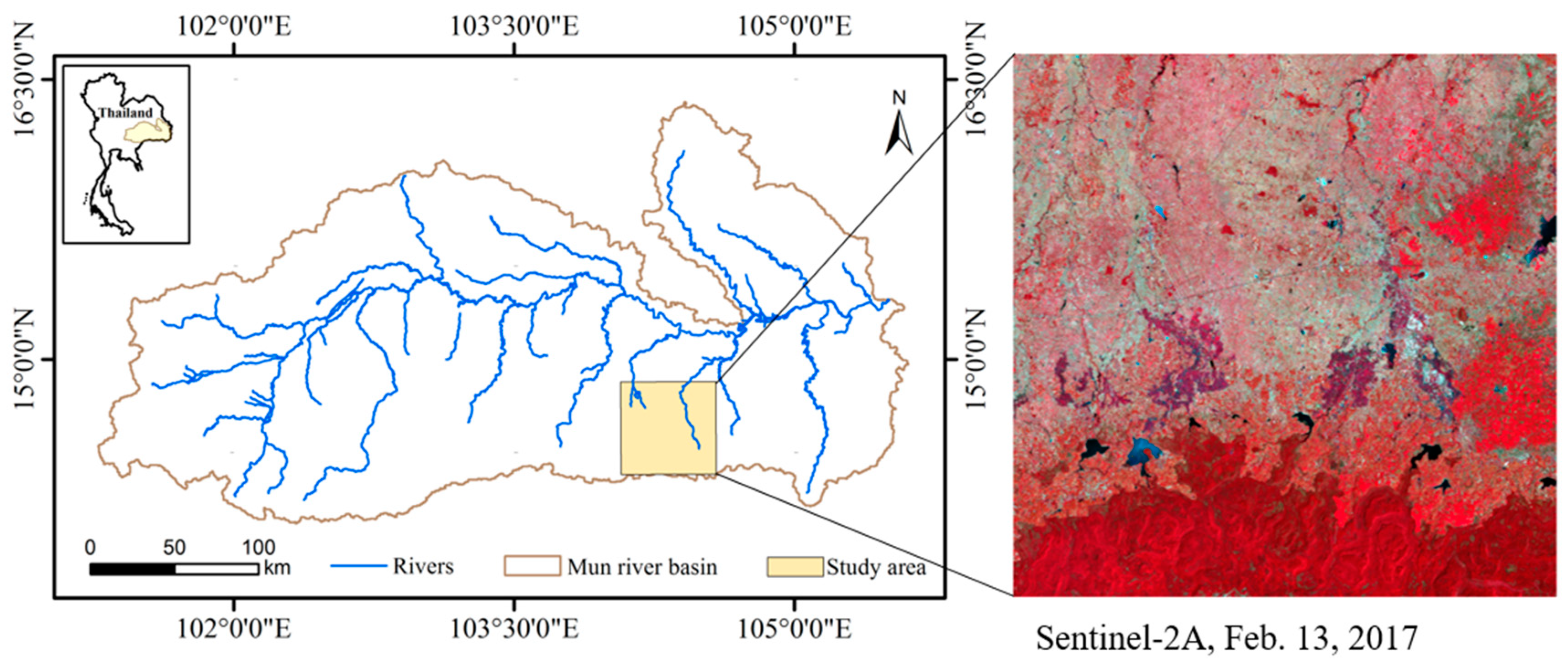
2.1. Study Area
2.2. Data and Preprocessing
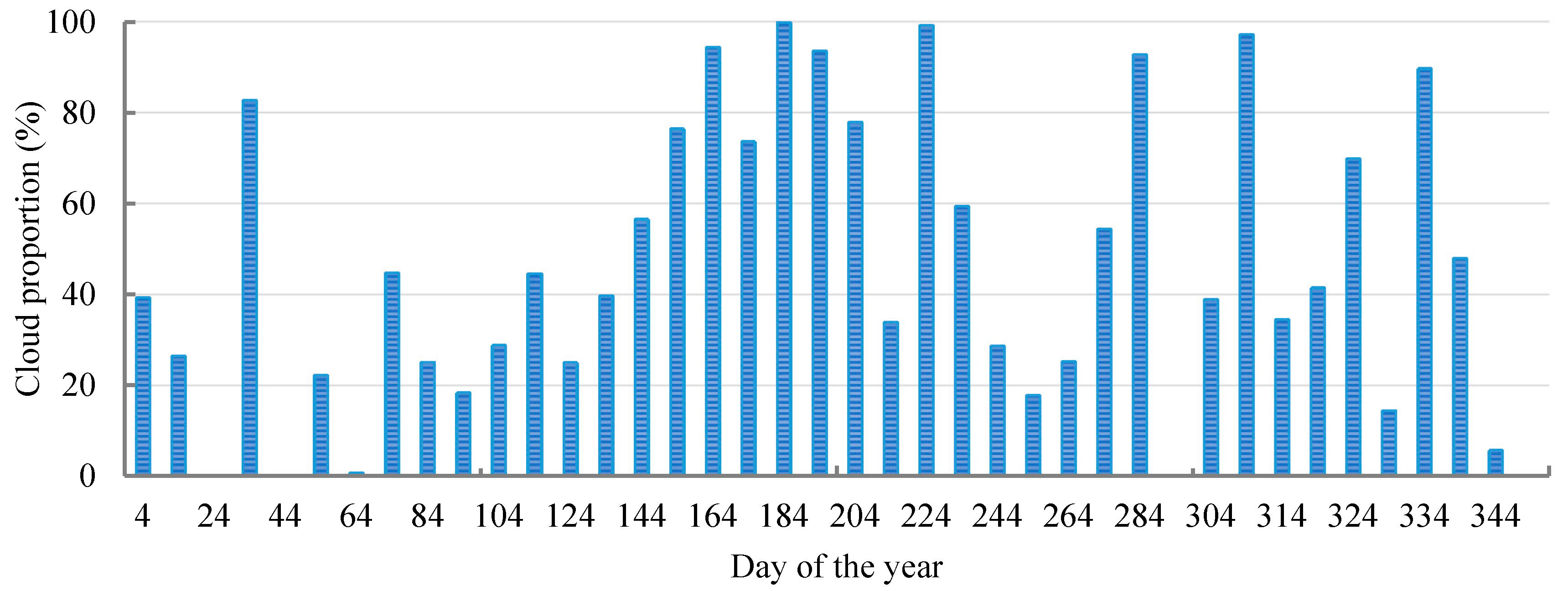
2.2.1. Sentinel-2 Single-Date Image Data
2.2.2. Stacking Time-Series Sentinel-2 NDVI
2.2.3. Ground Survey Data and Sample Datasets
2.3. Methods
2.3.1. Spectral and Textural Feature Analysis
2.3.2. Time-Series NDVI Statistical Indicator Analysis
- (1)
- NDVI_meanThe mean value reflects the concentrated trend in time-series NDVI data. The time-series dataset is represented as . N is the length of X, and the mean value () of X is calculated by
- (2)
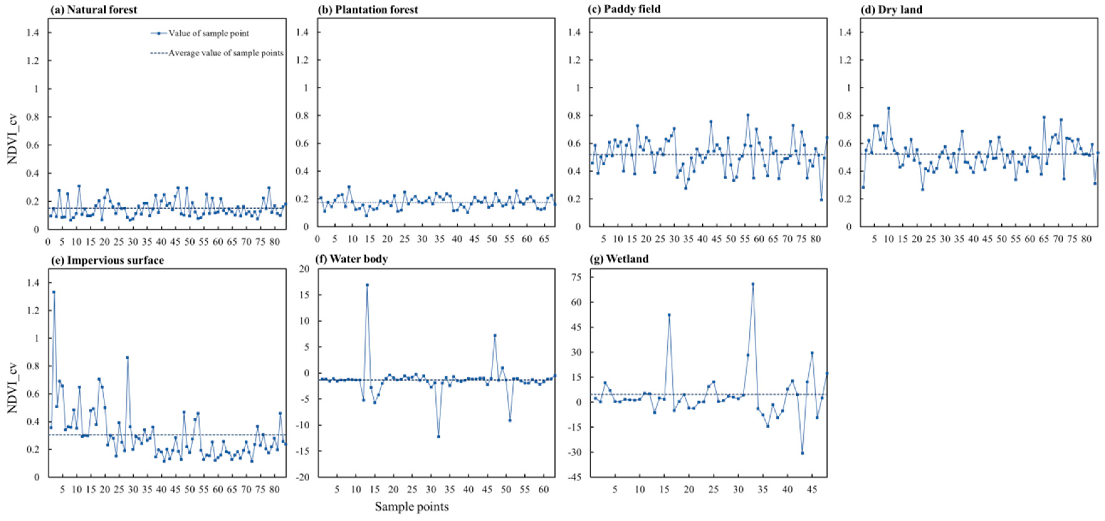
- NDVI_cvThe coefficient of variation reflects the dispersion degree and concentrated tendency of time-series NDVI data. This value is influenced by both the dispersion degree and the average population level. It is calculated bywhere is the mean value of the time-series data, and represents the standard deviation and reflects the dispersion degree of time-series data. is calculated asBoth NDVI_mean and NDVI_cv were calculated for each pixel based on NDVI time-series stack data within a Python development environment.
2.3.3. Random Forest Classification
2.3.4. Accuracy Assessment
3. Results
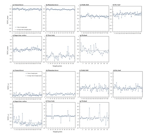
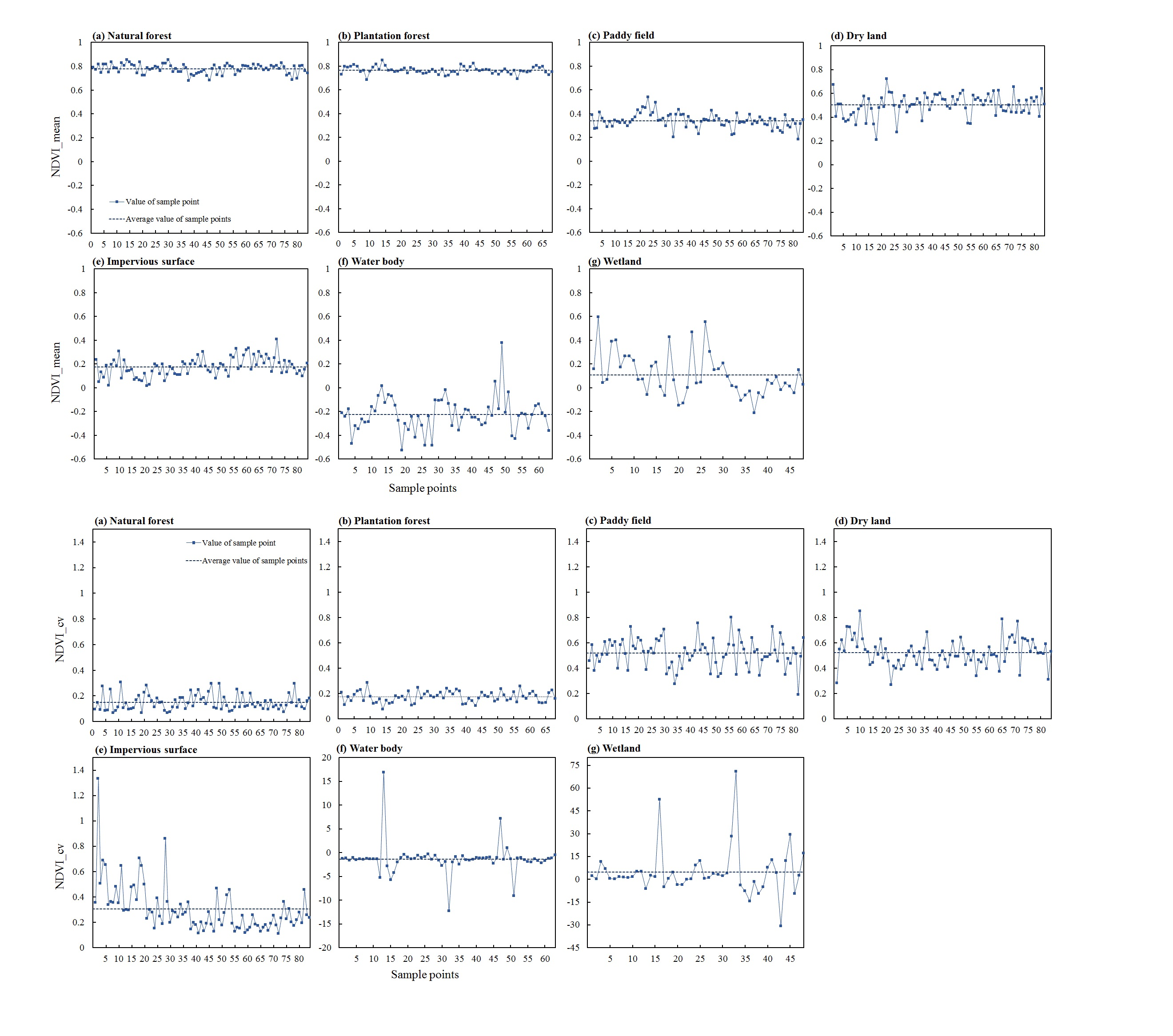
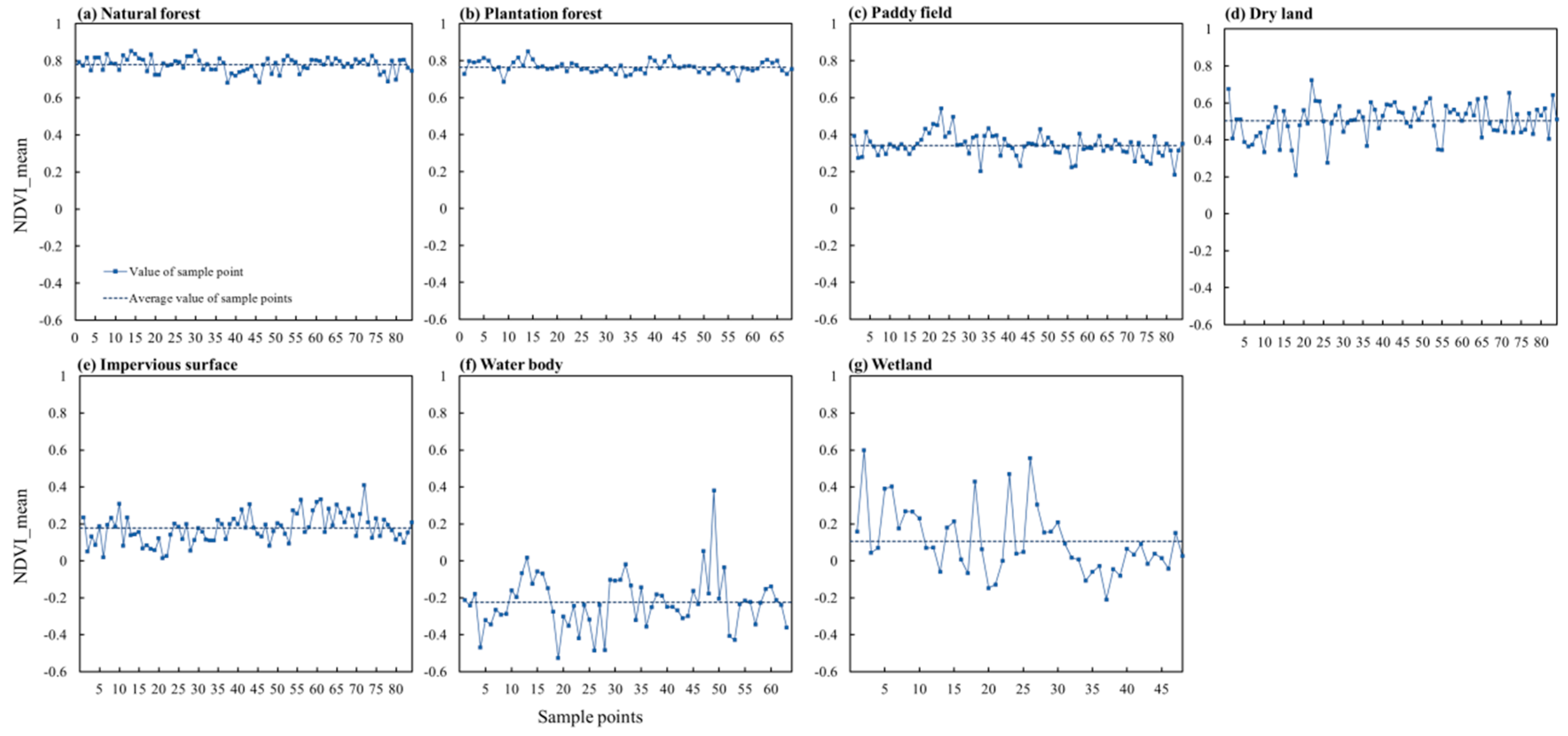
3.1. Separability of NDVI_mean and NDVI_cv for Different Land Cover Types
3.1.1. NDVI_mean
3.1.2. NDVI_cv
3.2. The Importance of Different Features
3.3. Comparison of Classification Results from Different Feature Combinations
- Spectral bands only (SB)
- Spectral bands and textural features (SBT)
- Spectral bands, textural features, and NDVI_mean (SBTM)
- Spectral bands, textural features, and NDVI_cv (SBTC)
- Spectral bands, textural features, and NDVI_mean + NDVI_cv (SBTMC)
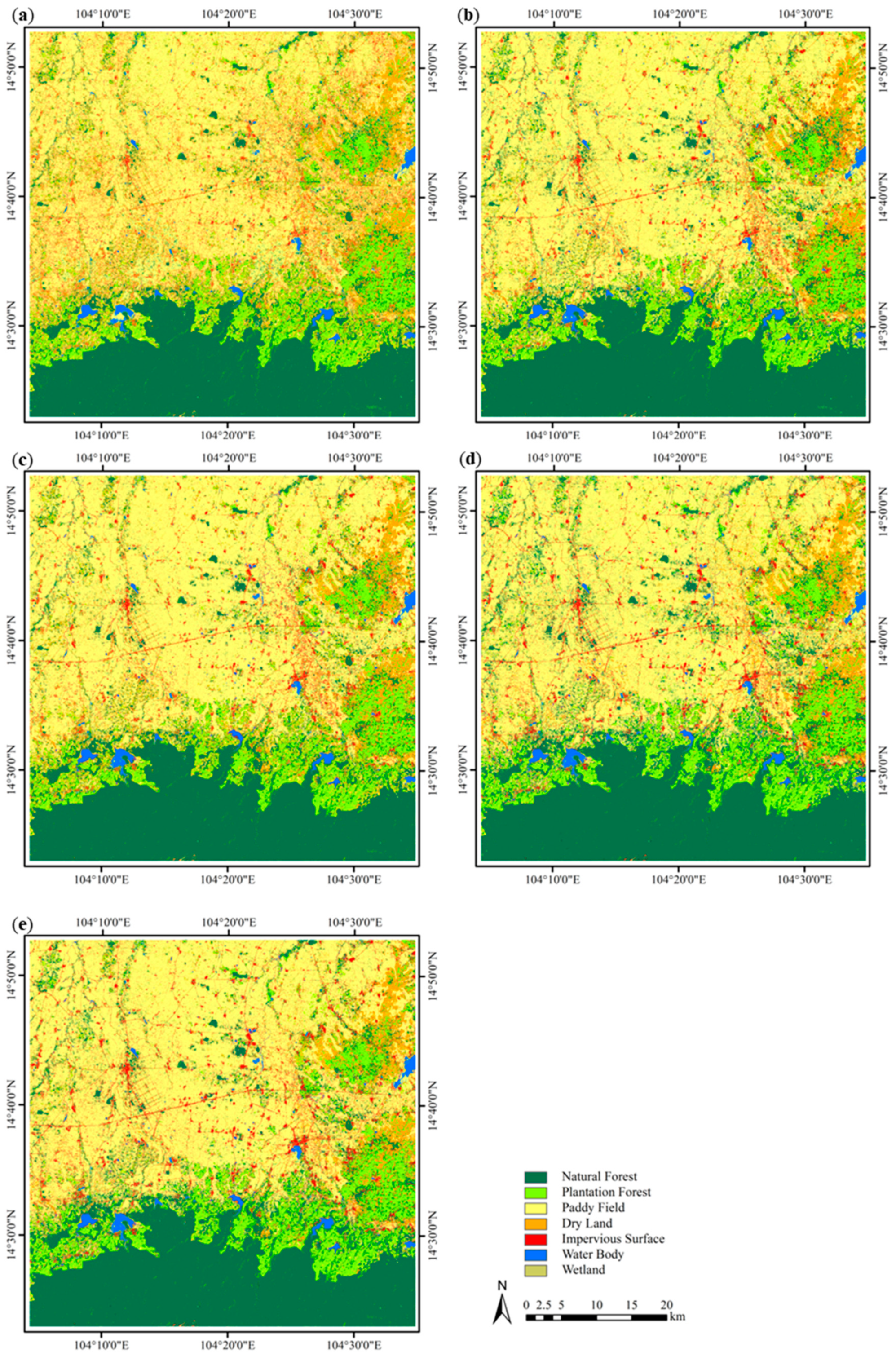
3.3.1. Spectral Bands Only (SB)
3.3.2. Spectral Bands and Textural Features (SBT)
3.3.3. SBT+NDVI_mean (SBTM) and SBT+NDVI_cv (SBTC)
3.3.4. SBT+NDVI_mean+NDVI_cv (SBTMC)
4. Discussion
4.1. The Advantages of Statistical Indicators for Land Cover Classification in Cloud-Prone Regions
4.2. Difficulty in Land Cover Classification at Fine Scales
4.2.1. Natural Forest vs. Plantation Forest
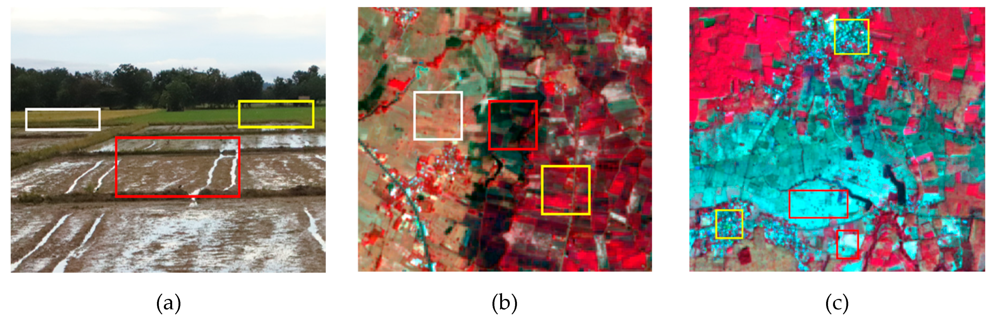
4.2.2. Paddy Field vs. Dry Field
4.2.3. Wetlands vs. Others
4.3. Uncertainty in Feature Importance Measures of the Random Forest Model
5. Conclusions
Author Contributions
Funding
Conflicts of Interest
References
- Bounoua, L.; DeFries, R.; Collatz, G.J.; Sellers, P.; Khan, H. Effects of land cover conversion on surface climate. Clim. Chang. 2002, 52, 29–64. [Google Scholar] [CrossRef]
- Herold, M.; Mayaux, P.; Woodcock, C.; Baccini, A.; Schmullius, C. Some challenges in global land cover mapping: An assessment of agreement and accuracy in existing 1 km datasets. Remote Sens. Environ. 2008, 112, 2538–2556. [Google Scholar] [CrossRef]
- Running, S.W. Ecosystem disturbance, carbon, and climate. Science 2008, 321, 652–653. [Google Scholar] [CrossRef]
- Gómez, C.; White, J.C.; Wulder, M.A. Optical remotely sensed time series data for land cover classification: A review. ISPRS J. Photogramm. Remote Sens. 2016, 116, 55–72. [Google Scholar] [CrossRef]
- Deng, C.; Wu, C. The use of single-date MODIS imagery for estimating large-scale urban impervious surface fraction with spectral mixture analysis and machine learning techniques. ISPRS J. Photogramm. Remote Sens. 2013, 86, 100–110. [Google Scholar] [CrossRef]
- Shoko, C.; Mutanga, O. Examining the strength of the newly-launched Sentinel 2 MSI sensor in detecting and discriminating subtle differences between C3 and C4 grass species. ISPRS J. Photogramm. Remote Sens. 2017, 129, 32–40. [Google Scholar] [CrossRef]
- Csillik, O.; Belgiu, M.; Asner, G.P.; Kelly, M. Object-based time-constrained dynamic time warping classification of crops using Sentinel-2. Remote Sens. 2019, 11, 1257. [Google Scholar] [CrossRef]
- Griffiths, P.; Nendel, C.; Hostert, P. Intra-annual reflectance composites from Sentinel-2 and Landsat for national-scale crop and land cover mapping. Remote Sens. Environ. 2019, 220, 135–151. [Google Scholar] [CrossRef]
- Hansen, M.C.; Potapov, P.V.; Moore, R.; Hancher, M.; Turubanova, S.A.; Tyukavina, A.; Thau, D.; Stehman, S.; Goetz, S.J.; Loveland, T.R. High-resolution global maps of 21st-century forest cover change. Science 2013, 342, 850–853. [Google Scholar] [CrossRef]
- Ludwig, C.; Walli, A.; Schleicher, C.; Weichselbaum, J.; Riffler, M. A highly automated algorithm for wetland detection using multi-temporal optical satellite data. Remote Sens. Environ. 2019, 224, 333–351. [Google Scholar] [CrossRef]
- Vuolo, F.; Neuwirth, M.; Immitzer, M.; Atzberger, C.; Ng, W.-T. How much does multi-temporal Sentinel-2 data improve crop type classification? Int. J. Appl. Earth Obs. Geoinf. 2018, 72, 122–130. [Google Scholar] [CrossRef]
- Khatami, R.; Mountrakis, G.; Stehman, S.V. A meta-analysis of remote sensing research on supervised pixel-based land-cover image classification processes: General guidelines for practitioners and future research. Remote Sens. Environ. 2016, 177, 89–100. [Google Scholar] [CrossRef]
- Parmentier, B.; Eastman, J.R. Land transitions from multivariate time series: Using seasonal trend analysis and segmentation to detect land-cover changes. Int. J. Remote Sens. 2014, 35, 671–692. [Google Scholar] [CrossRef]
- Sexton, J.O.; Urban, D.L.; Donohue, M.J.; Song, C. Long-term land cover dynamics by multi-temporal classification across the Landsat-5 record. Remote Sens. Environ. 2013, 128, 246–258. [Google Scholar] [CrossRef]
- Shao, Y.; Lunetta, R.S.; Wheeler, B.; Iiames, J.S.; Campbell, J.B. An evaluation of time-series smoothing algorithms for land-cover classifications using MODIS-NDVI multi-temporal data. Remote Sens. Environ. 2016, 174, 258–265. [Google Scholar] [CrossRef]
- Guan, X.; Huang, C.; Liu, G.; Meng, X.; Liu, Q. Mapping rice cropping systems in Vietnam using an NDVI-based time-series similarity measurement based on DTW distance. Remote Sens. 2016, 8, 19. [Google Scholar] [CrossRef]
- Jia, K.; Liang, S.; Zhang, N.; Wei, X.; Gu, X.; Zhao, X.; Yao, Y.; Xie, X. Land cover classification of finer resolution remote sensing data integrating temporal features from time series coarser resolution data. ISPRS J. Photogramm. Remote Sens. 2014, 93, 49–55. [Google Scholar] [CrossRef]
- Loveland, T.R.; Reed, B.C.; Brown, J.F.; Ohlen, D.O.; Zhu, Z.; Yang, L.; Merchant, J.W. Development of a global land cover characteristics database and IGBP DISCover from 1 km AVHRR data. Int. J. Remote Sens. 2000, 21, 1303–1330. [Google Scholar] [CrossRef]
- Xiao, X.; Boles, S.; Liu, J.; Zhuang, D.; Liu, M. Characterization of forest types in Northeastern China, using multi-temporal SPOT-4 VEGETATION sensor data. Remote Sens. Environ. 2002, 82, 335–348. [Google Scholar] [CrossRef]
- Immitzer, M.; Vuolo, F.; Atzberger, C. First experience with Sentinel-2 data for crop and tree species classifications in central Europe. Remote Sens. 2016, 8, 166. [Google Scholar] [CrossRef]
- Rujoiu-Mare, M.-R.; Olariu, B.; Mihai, B.-A.; Nistor, C.; Săvulescu, I. Land cover classification in Romanian Carpathians and Subcarpathians using multi-date Sentinel-2 remote sensing imagery. Eur. J. Remote Sens. 2017, 50, 496–508. [Google Scholar] [CrossRef]
- Rapinel, S.; Mony, C.; Lecoq, L.; Clement, B.; Thomas, A.; Hubert-Moy, L. Evaluation of Sentinel-2 time-series for mapping floodplain grassland plant communities. Remote Sens. Environ. 2019, 223, 115–129. [Google Scholar] [CrossRef]
- Hościło, A.; Lewandowska, A. Mapping forest type and tree species on a regional scale using multi-temporal Sentinel-2 data. Remote Sens. 2019, 11, 929. [Google Scholar] [CrossRef]
- Belgiu, M.; Csillik, O. Sentinel-2 cropland mapping using pixel-based and object-based time-weighted dynamic time warping analysis. Remote Sens. Environ. 2018, 204, 509–523. [Google Scholar] [CrossRef]
- Leinenkugel, P.; Wolters, M.L.; Kuenzer, C.; Oppelt, N.; Dech, S. Sensitivity analysis for predicting continuous fields of tree-cover and fractional land-cover distributions in cloud-prone areas. Int. J. Remote Sens. 2014, 35, 2799–2821. [Google Scholar] [CrossRef]
- Petitjean, F.; Inglada, J.; Gançarski, P. Satellite image time series analysis under time warping. IEEE Trans. Geosci. Remote Sens. 2012, 50, 3081–3095. [Google Scholar] [CrossRef]
- Leinenkugel, P.; Kuenzer, C.; Oppelt, N.; Dech, S. Characterisation of land surface phenology and land cover based on moderate resolution satellite data in cloud prone areas—A novel product for the Mekong Basin. Remote Sens. Environ. 2013, 136, 180–198. [Google Scholar] [CrossRef]
- Torbick, N.; Ledoux, L.; Salas, W.; Zhao, M. Regional mapping of plantation extent using multisensor imagery. Remote Sens. 2016, 8, 236. [Google Scholar] [CrossRef]
- Zhao, Z.; Liu, G.; Liu, Q.; Huang, C.; Li, H.; Wu, C. Distribution characteristics and seasonal variation of soil nutrients in the Mun River Basin, Thailand. Int. J. Environ. Res. Public Health 2018, 15, 1818. [Google Scholar] [CrossRef]
- Guan, X.; Liu, G.; Huang, C.; Meng, X.; Liu, Q.; Wu, C.; Ablat, X.; Chen, Z.; Wang, Q. An Open-Boundary Locally Weighted Dynamic Time Warping Method for Cropland Mapping. ISPRS Int. J. Geo-Inf. 2018, 7, 75. [Google Scholar] [CrossRef]
- Chatziantoniou, A.; Psomiadis, E.; Petropoulos, G.P. Co-Orbital Sentinel 1 and 2 for LULC mapping with emphasis on wetlands in a mediterranean setting based on machine learning. Remote Sens. 2017, 9, 1259. [Google Scholar] [CrossRef]
- Louis, J.; Debaecker, V.; Pflug, B.; Main-Knorn, M.; Bieniarz, J.; Mueller-Wilm, U.; Cadau, E.; Gascon, F. Sentinel-2 Sen2Cor: L2A processor for users. In Proceedings of the Living Planet Symposium 2016, Prague, Czech, 9–13 May 2016. Spacebooks Online. [Google Scholar]
- Exelis, V. ENVI 5.3; Exelis VIS: Boulder, CO, USA, 2015. [Google Scholar]
- Yu, L.; Gong, P. Google Earth as a virtual globe tool for Earth science applications at the global scale: Progress and perspectives. Int. J. Remote Sens. 2012, 33, 3966–3986. [Google Scholar] [CrossRef]
- Price, M.H. Mastering ArcGIS; McGraw-Hill: New York, NY, USA, 2010. [Google Scholar]
- Haralick, R.M.; Shanmugam, K.; Dinstein, I.H. Textural features for image classification. IEEE Trans. Syst. ManCybern. 1973, 610–621. [Google Scholar] [CrossRef]
- Jensen, J.R. Introductory Digital Image Processing: A Remote Sensing Perspective, 4th ed.; Pearson Education: Glenview, IL, USA, 2016. [Google Scholar]
- Breiman, L. Random forests. Mach. Learn. 2001, 45, 5–32. [Google Scholar] [CrossRef]
- Belgiu, M.; Drăguţ, L. Random forest in remote sensing: A review of applications and future directions. ISPRS J. Photogramm. Remote Sens. 2016, 114, 24–31. [Google Scholar] [CrossRef]
- Rodriguez-Galiano, V.F.; Ghimire, B.; Rogan, J.; Chica-Olmo, M.; Rigol-Sanchez, J.P. An assessment of the effectiveness of a random forest classifier for land-cover classification. ISPRS J. Photogramm. Remote Sens. 2012, 67, 93–104. [Google Scholar] [CrossRef]
- Li, M.; Ma, L.; Blaschke, T.; Cheng, L.; Tiede, D. A systematic comparison of different object-based classification techniques using high spatial resolution imagery in agricultural environments. Int. J. Appl. Earth Obs. Geoinf. 2016, 49, 87–98. [Google Scholar] [CrossRef]
- Warmerdam, F. The Geospatial Data Abstraction Library, in Open Source Approaches in Spatial Data Handling; Springer: Berlin/Heidelberg, Germany, 2008; pp. 87–104. [Google Scholar]
- Gislason, P.O.; Benediktsson, J.A.; Sveinsson, J.R. Random forests for land cover classification. Pattern Recognit. Lett. 2006, 27, 294–300. [Google Scholar] [CrossRef]
- Foody, G.M. Status of land cover classification accuracy assessment. Remote Sens. Environ. 2002, 80, 185–201. [Google Scholar] [CrossRef]
- Congalton, R.G. A review of assessing the accuracy of classifications of remotely sensed data. Remote Sens. Environ. 1991, 37, 35–46. [Google Scholar] [CrossRef]
- Cohen, J. A coefficient of agreement for nominal scales. Educ. Psychol. Meas. 1960, 20, 37–46. [Google Scholar] [CrossRef]
- Brown, J.C.; Kastens, J.H.; Coutinho, A.C.; de Castro Victoria, D.; Bishop, C.R. Classifying multiyear agricultural land use data from Mato Grosso using time-series MODIS vegetation index data. Remote Sens. Environ. 2013, 130, 39–50. [Google Scholar] [CrossRef]
- Basnet, B.; Vodacek, A. Tracking land use/land cover dynamics in cloud prone areas using moderate resolution satellite data: A case study in Central Africa. Remote Sens. 2015, 7, 6683–6709. [Google Scholar] [CrossRef]
- Ju, J.; Roy, D.P. The availability of cloud-free Landsat ETM+ data over the conterminous United States and globally. Remote Sens. Environ. 2008, 112, 1196–1211. [Google Scholar] [CrossRef]
- Miettinen, J.; Liew, S.C. Separability of insular Southeast Asian woody plantation species in the 50 m resolution ALOS PALSAR mosaic product. Remote Sens. Lett. 2011, 2, 299–307. [Google Scholar] [CrossRef]
- Culbert, P.D.; Pidgeon, A.M.; Louis, V.S.; Bash, D.; Radeloff, V.C. The impact of phenological variation on texture measures of remotely sensed imagery. IEEE J. Sel. Top. Appl. Earth Obs. Remote Sens. 2009, 2, 299–309. [Google Scholar] [CrossRef]
- Dian, Y.; Li, Z.; Pang, Y. Spectral and texture features combined for forest tree species classification with airborne hyperspectral imagery. J. Indian Soc. Remote Sens. 2015, 43, 101–107. [Google Scholar] [CrossRef]
- Xiao, X.; Boles, S.; Liu, J.; Zhuang, D.; Frolking, S.; Li, C.; Salas, W.; Moore, B., III. Mapping paddy rice agriculture in southern China using multi-temporal MODIS images. Remote Sens. Environ. 2005, 95, 480–492. [Google Scholar] [CrossRef]
- Park, S.; Im, J.; Park, S.; Yoo, C.; Han, H.; Rhee, J. Classification and mapping of paddy rice by combining Landsat and SAR time series data. Remote Sens. 2018, 10, 447. [Google Scholar] [CrossRef]
- Wang, D.; Wan, B.; Qiu, P.; Su, Y.; Guo, Q.; Wang, R.; Sun, F.; Wu, X. Evaluating the performance of sentinel-2, landsat 8 and pléiades-1 in mapping mangrove extent and species. Remote Sens. 2018, 10, 1468. [Google Scholar] [CrossRef]
- Zhu, J.; Pan, Z.; Wang, H.; Huang, P.; Sun, J.; Qin, F.; Liu, Z. An Improved Multi-temporal and Multi-feature Tea Plantation Identification Method Using Sentinel-2 Imagery. Sensors 2019, 19, 2087. [Google Scholar] [CrossRef] [PubMed]
- Ramoelo, A.; Cho, M.; Mathieu, R.; Skidmore, A.K. Potential of Sentinel-2 spectral configuration to assess rangeland quality. J. Appl. Remote Sens. 2015, 9, 094096. [Google Scholar] [CrossRef]
- Schultz, B.; Immitzer, M.; Formaggio, A.R.; Sanches, I.D.A.; Luiz, A.J.B.; Atzberger, C. Self-guided segmentation and classification of multi-temporal Landsat 8 images for crop type mapping in Southeastern Brazil. Remote Sens. 2015, 7, 14482–14508. [Google Scholar] [CrossRef]
- Schuster, C.; Förster, M.; Kleinschmit, B. Testing the red edge channel for improving land-use classifications based on high-resolution multi-spectral satellite data. Int. J. Remote Sens. 2012, 33, 5583–5599. [Google Scholar] [CrossRef]


| No. | Features | Importance | OOB accuracy | No. | Features | Importance | OOB accuracy |
|---|---|---|---|---|---|---|---|
| 1 | NIR-2 | 0.10050 | 0.72482 | 12 | NIR-1 | 0.04578 | 0.99751 |
| 2 | Red edge-1 | 0.09822 | 0.91278 | 13 | NDVI_cv | 0.04481 | 0.99748 |
| 3 | Red | 0.07824 | 0.94389 | 14 | Red edge-2 | 0.04001 | 0.99788 |
| 4 | NDVI_mean | 0.07004 | 0.98054 | 15 | ENT _2 | 0.02297 | 0.99788 |
| 5 | Green | 0.06544 | 0.98764 | 16 | ASM _1 | 0.01926 | 0.99788 |
| 6 | MEAN_1 | 0.06429 | 0.99484 | 17 | ASM _2 | 0.01536 | 0.99777 |
| 7 | SWIR-1 | 0.06116 | 0.99580 | 18 | CON _2 | 0.01193 | 0.99788 |
| 8 | Red edge-3 | 0.06111 | 0.99696 | 19 | ENT _1 | 0.01141 | 0.99799 |
| 9 | MEAN_2 | 0.05809 | 0.99699 | 20 | COR_2 | 0.01046 | 0.99803 |
| 10 | SWIR-2 | 0.05230 | 0.99710 | 21 | COR_1 | 0.01029 | 0.99807 |
| 11 | Blue | 0.04825 | 0.99740 | 22 | CON_1 | 0.01008 | 0.99803 |
| Natural forest | Plantation forest | Paddy field | Dry field | Water body | Wetland | Impervious surface | Producer’s accuracy | |
|---|---|---|---|---|---|---|---|---|
| Natural forest | 900 | 36 | 45 | 28 | 18 | 87.63% | ||
| Plantation forest | 69 | 479 | 34 | 27 | 2 | 78.40% | ||
| Paddy field | 45 | 31 | 1427 | 105 | 116 | 82.77% | ||
| Dry field | 22 | 28 | 33 | 241 | 5 | 73.25% | ||
| Water body | 13 | 76 | 1 | 84.44% | ||||
| Wetland | 1 | 11 | 5 | 14 | 45.16% | |||
| Impervious surface | 6 | 87 | 37 | 188 | 59.12% | |||
| User’s accuracy | 86.29% | 83.45% | 86.48% | 55.02% | 93.83% | 100.00% | 56.97% |
| Natural forest | Plantation forest | Paddy field | Dry field | Water body | Wetland | Impervious surface | Producer’s accuracy | |
|---|---|---|---|---|---|---|---|---|
| Natural forest | 917 | 17 | 57 | 34 | 2 | 89.29% | ||
| Plantation forest | 66 | 494 | 25 | 26 | 80.85% | |||
| Paddy field | 58 | 7 | 1516 | 91 | 52 | 87.94% | ||
| Dry field | 21 | 22 | 25 | 250 | 11 | 75.99% | ||
| Water body | 3 | 85 | 2 | 94.44% | ||||
| Wetland | 20 | 2 | 9 | 29.03% | ||||
| Impervious surface | 5 | 41 | 14 | 258 | 81.13% | |||
| User’s accuracy | 85.94% | 91.48% | 89.86% | 60.24% | 97.70% | 100.00% | 79.38% |
| Natural forest | Plantation forest | Paddy field | Dry field | Water body | Wetland | Impervious surface | Producer’s accuracy | |
|---|---|---|---|---|---|---|---|---|
| Natural forest | 916 | 23 | 42 | 44 | 2 | 89.19% | ||
| Plantation forest | 59 | 501 | 21 | 30 | 82.00% | |||
| Paddy field | 35 | 2 | 1552 | 77 | 58 | 90.02% | ||
| Dry field | 21 | 22 | 25 | 256 | 5 | 77.81% | ||
| Water body | 2 | 85 | 3 | 94.44% | ||||
| wetland | 15 | 5 | 11 | 35.48% | ||||
| Impervious surface | 4 | 36 | 12 | 266 | 83.65% | |||
| User’s accuracy | 88.50% | 91.42% | 91.67% | 61.10% | 94.44% | 100.00% | 79.64% |
| Natural forest | Plantation forest | Paddy field | Dry field | Water body | Wetland | Impervious surface | Producer’s accuracy | |
|---|---|---|---|---|---|---|---|---|
| Natural forest | 930 | 27 | 50 | 10 | 10 | 90.56% | ||
| Plantation forest | 70 | 515 | 20 | 6 | 84.29% | |||
| Paddy field | 74 | 4 | 1512 | 86 | 48 | 87.70% | ||
| Dry field | 20 | 24 | 26 | 253 | 6 | 76.90% | ||
| Water body | 4 | 1 | 84 | 1 | 93.33% | |||
| Wetland | 9 | 11 | 11 | 35.48% | ||||
| Impervious surface | 6 | 11 | 7 | 294 | 92.45% | |||
| User’s accuracy | 84.55% | 90.35% | 92.65% | 69.70% | 88.42% | 100.00% | 81.89% |
| Natural forest | Plantation forest | Paddy field | Dry field | Water body | Wetland | Impervious surface | Producer’s accuracy | |
|---|---|---|---|---|---|---|---|---|
| Natural forest | 941 | 26 | 38 | 17 | 5 | 91.63% | ||
| Plantation forest | 68 | 514 | 19 | 10 | 84.12% | |||
| Paddy field | 45 | 4 | 1569 | 57 | 49 | 91.01% | ||
| Dry field | 19 | 20 | 28 | 258 | 4 | 78.42% | ||
| Water body | 3 | 85 | 2 | 94.44% | ||||
| Wetland | 10 | 5 | 16 | 51.61% | ||||
| Impervious surface | 5 | 10 | 5 | 298 | 93.71% | |||
| User’s Accuracy | 87.29% | 91.13% | 93.56% | 74.35% | 94.44% | 100.00% | 83.24% |
© 2020 by the authors. Licensee MDPI, Basel, Switzerland. This article is an open access article distributed under the terms and conditions of the Creative Commons Attribution (CC BY) license (http://creativecommons.org/licenses/by/4.0/).
Share and Cite
Huang, C.; Zhang, C.; He, Y.; Liu, Q.; Li, H.; Su, F.; Liu, G.; Bridhikitti, A. Land Cover Mapping in Cloud-Prone Tropical Areas Using Sentinel-2 Data: Integrating Spectral Features with Ndvi Temporal Dynamics. Remote Sens. 2020, 12, 1163. https://doi.org/10.3390/rs12071163
Huang C, Zhang C, He Y, Liu Q, Li H, Su F, Liu G, Bridhikitti A. Land Cover Mapping in Cloud-Prone Tropical Areas Using Sentinel-2 Data: Integrating Spectral Features with Ndvi Temporal Dynamics. Remote Sensing. 2020; 12(7):1163. https://doi.org/10.3390/rs12071163
Chicago/Turabian StyleHuang, Chong, Chenchen Zhang, Yun He, Qingsheng Liu, He Li, Fenzhen Su, Gaohuan Liu, and Arika Bridhikitti. 2020. "Land Cover Mapping in Cloud-Prone Tropical Areas Using Sentinel-2 Data: Integrating Spectral Features with Ndvi Temporal Dynamics" Remote Sensing 12, no. 7: 1163. https://doi.org/10.3390/rs12071163
APA StyleHuang, C., Zhang, C., He, Y., Liu, Q., Li, H., Su, F., Liu, G., & Bridhikitti, A. (2020). Land Cover Mapping in Cloud-Prone Tropical Areas Using Sentinel-2 Data: Integrating Spectral Features with Ndvi Temporal Dynamics. Remote Sensing, 12(7), 1163. https://doi.org/10.3390/rs12071163