Magnetospheric–Ionospheric–Lithospheric Coupling Model. 1: Observations during the 5 August 2018 Bayan Earthquake

Abstract

The short-term prediction of earthquakes is an essential issue connected with human life protection and related social and economic matters. Recent papers have provided some evidence of the link between the lithosphere, lower atmosphere, and ionosphere, even though with marginal statistical evidence. The basic coupling is hypothesized as being via the atmospheric gravity wave (AGW)/acoustic wave (AW) channel. In this paper we analyze a scenario of the low latitude earthquake (Mw = 6.9) which occurred in Indonesia on 5 August 2018, through a multi-instrumental approach, using ground and satellites high quality data. As a result, we derive a new analytical lithospheric–atmospheric–ionospheric–magnetospheric coupling model with the aim to provide quantitative indicators to interpret the observations around 6 h before and at the moment of the earthquake occurrence.

1. Introduction

In the last few years, there has been an increasing interest in the scientific community towards the short-term forecasting of earthquakes (EQs), since many anomalies, statistically correlated with a seismic activity, have been found in the atmosphere and ionosphere, rather than in the lithosphere [1,2,3]. Ionospheric plasma density perturbations, occurring in its lower-side [4], as well as in its upper-side [5], give the most promising results. As a consequence, a few hypotheses have been introduced in order to justify the coupling among lithosphere, atmosphere and ionosphere. The first one, which is based on the chemical transmission, hypothesizes that the atmospheric conductivity can be perturbed by radon outflow close to the earthquake epicenter (EE), leading to a modification of the atmospheric electric field that drives a variation in the ionospheric plasma density profile [6,7,8]. The second one is based on the emission of atmospheric acoustic gravity waves (AGWs). Namely, such oscillations, developing around the EE, perturb the atmosphere in terms of changes in temperature, pressure, ground motion, etc. AGWs can propagate upward and, thus, can drive disturbances in the ionosphere [9,10,11,12]. The third one is electrostatic transmission. Basically, an electrostatic effect is produced in the lithosphere and released in the lower atmosphere by “stress-induced positive holes” which alter the ionospheric ionization status [13,14]. Nonetheless, because of the insufficient amount of experimental evidence supporting those theories, there are many other aspects of the lithosphere–atmosphere–ionosphere coupling process that cannot be explained yet [3,15,16]. In this scenario, models based on AGWs emission seems to provide the most promising results to correctly understand the lithosphere–atmosphere–ionosphere coupling processes in concomitance with an EQ. In fact, many studies using sub-ionospheric soundings through very low frequency/extreme low frequency band before and during a seismic event support the AGW hypothesis—e.g., in [2,4,9,11,17]. Anyway, it has to be stressed that all these observations give no information on the lithosphere/atmosphere coupling mechanisms, since only the lower ionosphere is studied. As a consequence, in recent years, many works hunted for a possible link in the lithosphere–atmosphere–ionosphere system during active seismic conditions. The authors in Korepanov et al. [18], investigating surface atmospheric pressure and magnetic field data during meteorological events, concluded that AGWs are a possible candidate for seismo-ionospheric coupling. A similar study by Nakamura et al. [19] for the 2004 Niigata-Chuetsu EQ (M6.8), using wavelet analyses, confirmed that enhanced variations in the period of 10–100 min of the surface atmospheric pressure and magnetic field data (which are in the range of AGW) enhanced the lower ionosphere perturbation. The authors in Endo et al. [20], using the Japanese F-net wide-band seismic network data, found that, before the 2007 Niigata-Chuetsu Oki and 2008 Iwate-Miyagi EQs, the ground motions in the AGW ranges were enhanced when the lower ionosphere was perturbed. Moreover, the analysis of the crustal motion based on the Global Positioning System data during the 2011 Tohoku EQ suggested a direct time-correlation with very low frequency/extreme low frequency sub-ionospheric and ultra-low frequency magnetic field variations—e.g., in [21,22,23,24]. To conclude, the literature mentioned above provides some evidence on the coupling among lithosphere, lower atmosphere, and ionosphere via the AGW channel.

The present paper, has a two fold approach: on the one hand, it shows the detailed investigation of a Mw 6.9 low latitude earthquake, registered in Indonesia on 5 August 2018, at 11:46 UT, based on a multi-instrumental analysis, using both ground and satellite data; on the other hand, it provides a new analytical magnetospheric–ionospheric–lithospheric coupling model, allowing us, for the first time, to quantitatively explain the experimental observations $\sim 6$ h before and at the moment of the earthquake occurrence. The manuscript is organized in the following way: Section 2 shows all the data and methods used for the entire analysis; Section 3 presents the analysis during the EQ occurrence; Section 4 displays the analysis $\sim 6$ h before the EQ; Section 5 discusses the results obtained and the main features of the new analytical model proposed; in Section 6 the conclusions are summarized.

2. Data and Methods

In the following section, we introduce the data set used and the techniques applied for the analysis.

2.1. Atmospheric Temperature and Acoustic Gravity Waves Evaluation

The atmospheric temperature profiles were retrieved from ERA5, which is the 5^th generation atmospheric data set produced by the European Centre for Medium-Range Weather Forecasts [25]. The model produces global and hourly temperature profiles with high resolution (137 different pressure levels) from near surface up to 0.01 hPa (∼80 km altitude) using observations from satellites, radiosondes, dropsondes, aircraft, and radars [25]. The horizontal resolution is ∼0.28${}^{\circ }$ in both longitude and latitude.

In this study, as a key indicator to estimate the AGW activity, we used the potential energy ($E_P$), which directly depends on the atmospheric vertical temperature profiles [26,27], that in the specific event were retrieved from ERA5. To evaluate $E_P$ values, we used the approach by Yang et al. [28,29]. The potential energy density [27] is defined as:

$$E_P=\frac{1}{2}{\left(\frac{g}{N}\right)}^2\overline{{\left(\frac{T^{\prime }}{\overline{T}}\right)}^2}$$

(1)

where g = 9.8 m/s${}^2$ is the gravitational acceleration (constant with altitude), N is the $Brunt-V\ddot{a}is\ddot{a}l\ddot{a}$ frequency, and $T^{\prime }$ is the fluctuations with respect to the background temperature $\overline{T}$. These three variables are functions of altitude z and were derived from the ERA5 profiles. To retrieve $\overline{T}$, we made a 2 km moving average. $T^{\prime }$ is obtained by subtracting $\overline{T}$ from the original temperature profile.

The term $\overline{{\left(\frac{T^{\prime }}{\overline{T}}\right)}^2}$, representing a variance, was evaluated within a layer of 2-km thickness, using the following equation:

$$\overline{{\left(\frac{T^{\prime }}{\overline{T}}\right)}^2}=\frac{1}{h^{max}-h^{min}}{\int }_{h_{min}}^{h_{max}}{\left(\frac{T^{\prime }}{\overline{T}}\right)}^{2}dh$$

(2)

where $h_{max}$ and $h_{min}$ represent the top and bottom altitudes of the layer, respectively.

2.2. The Vertical Total Electron Content (vTEC)

TEC is the total electron content for the line of sight, from the ground receiver to the GNSS satellite whose instrumentation, tracked by the non-profit university-governed consortium UNAVCO (https://www.unavco.org/), records broadcast signals from the satellite constellation used in this work. Specifically, we selected 13 International GNSS Service stations whose geographic coordinates are reported in

Table 1. Geographic location of the International GNSS Service stations used for the vTEC evaluation.

Site	City	Country	Latitude	Longitude
ALIC00AUS	Alice Springs	Australia	−23.67${}^{\circ }$	133.89${}^{\circ }$
BAKO00IDN	Cibinong	Indonesia	−6.49${}^{\circ }$	106.85${}^{\circ }$
BNOA00IDN	Benoa	Indonesia	−8.7465${}^{\circ }$	115.21${}^{\circ }$
BTNG00IDN	Bitung	Indonesia	1.4389${}^{\circ }$	125.19${}^{\circ }$
CIBG00IDN	Cibinong	Indonesia	−6.4904${}^{\circ }$	106.85${}^{\circ }$
DARW00AUS	Darwin	Australia	−12.8437${}^{\circ }$	131.13${}^{\circ }$
JOG200IDN	Yogyakarta	Indonesia	−7.7638${}^{\circ }$	110.37${}^{\circ }$
KAT100AUS	Katherine	Australia	−14.3760${}^{\circ }$	132.15${}^{\circ }$
MRO100AUS	Boolardy Station	Australia	−26.6966${}^{\circ }$	116.64${}^{\circ }$
NTUS00SGP	Singapore	Singapore	1.3458${}^{\circ }$	103.68${}^{\circ }$
PGEN00PHL	General Santos City	Philippines	6.0649${}^{\circ }$	125.13${}^{\circ }$
PPPC00PHL	Puerto Princesa City	Philippines	9.7729${}^{\circ }$	118.74${}^{\circ }$
XMIS00AUS	Christmas Island	Australia	−10.4499${}^{\circ }$	105.69${}^{\circ }$

, together with the receivers’ identifiers, the city and the country.

The raw data acquired were converted into standard daily RINEX files suitable for processing. Due to the dispersive nature of the ionosphere it was possible to calculate the TEC starting from the code or carrier phase measurements provided by GNSS receivers on different frequencies. TEC was assumed as the total number of free electrons in a cylinder with cross section of 1 m${}^2$ and height equal to the slant signal path. It was defined as the integral of the electron density ($N_e$) along the GNSS signal ray path (z), according to the following equation:

$$TEC={\int }_{satellite}^{receiver}{N}_{e}dz$$

(3)

This quantity can be calculated along each slant path according to the following equation:

$$TEC=\frac{1}{40.3}\left(\frac{f_1{f}_2}{f_1-f_2}\right)(P_2-P_1)-ϵ$$

(4)

Equation (4) describes the so-called geometry-free combination in which $f_1$ and $f_2$ are the two carrier frequencies of the transmitted signal. In more detail, for GNSS signals $f_1$ corresponds to $L_1$ (1575.42 MHz) and $f_2$ corresponds to $L_2$ (1227.60 MHz). $P_1$ and $P_2$ are the corresponding pseudoranges (i.e., the satellite-receiver optical path), while $ϵ$ represents all the frequency-dependent biases induced by the receiver, the satellite and the environment in which the measurement is carried out. As each TEC value obtained from Equation (4) is assimilated to the measure of the electron content along the satellite-receiver path, it is called slant TEC (sTEC). In this way, for each satellite and for each period, TEC measurements take place at different elevation angles and are related to different ionospheric sectors. However, according to the Equation (4), such TEC measurement are affected by biases. So, to minimize such biases, we used the GOPI calibration software (http://seemala.blogspot.it/2011/04/rinex-gps-tecprogram-version-22.html) that provides calibrated TEC values projected to the vertical (vTEC), by assuming the ionosphere as a single, thin, ionized layer located at 350 km [30]. The vertical projection is allowed to obtain TEC values that do not depend on the position of the GNSS receivers at ground. In this paper, the vTEC time series were calculated over each station in the period between 1 August to 10 August 2018, adopting the method described above. vTEC is expressed in units of 10${}^{16}$ m${}^{-2}=1TECu$. All the results are expressed in Universal Time (UT).

2.3. China Seismo-Electromagnetic Satellite (CSES) Data

CSES-01, a sun-synchronous satellite, flies at an altitude of ∼507 km [31], has an orbital descending node time at ∼14:00 LT (local time) and a revisiting period of 5 days. CSES-01 hosts nine payloads: a high-precision magnetometer (HPM) [32], a search coil magnetometer (SCM) [33], an electric field detector (EFD) [34], a Langmuir probe (LAP) [35], a plasma analyzer (PAP) [36], a high energetic particle package (HAPP) [37], an high-energy particle detector (HEPD) [38], a GNSS occultation receiver (GOR) [39], and a tri-band beacon (TBB) [40] to detect magnetospheric signals and perturbations induced from space and ground. In this study we used geomagnetic field (from SCM), electric field (from EFD) and electron density (from LAP) data. The EFD data are in the frequency band from direct current to 2 kHz with a sampling frequency of 2.5 kHz. SCM data are in the frequency band from 10 Hz to 2.2 kHz with a sampling frequency of 51 kHz. Both EFD and SCM vectors were analyzed under the geographical coordinate system. LAP data are sampled every 3 s.

2.4. Ground Magnetometer and Magnetospheric Field Line Resonance Frequency Estimation

The magnetometers at ground used for the present analysis come from the INTERMAGNET magnetometer array network, which is a consortium of observatories guaranteeing a common standard data release to the scientific community, leading to possible comparison among measurements at different observation points. In our analysis used 1 s resolution data from Gingin (GNG) ($\lambda =31.{36}^{\circ }$S and $\varphi =115.{71}^{\circ }$E, $\lambda$ and $\varphi$ being the geographical latitude and longitude, respectively) and Learmonth (LRM) ($\lambda =22.{22}^{\circ }$S and $\varphi =114.1^{\circ }$E).

To evaluate the geomagnetic Field line resonance (FLR) frequency, we used the well established gradient method [41,42,43,44], which relies on geomagnetic observations from a pair of magnetometers slightly separated in latitude and approximately aligned along the same magnetic meridian. The method takes advantage of the fact that the field lines connected to the two stations have similar frequency response, both in amplitude and phase, but are slightly shifted in frequency. In particular, the resonance frequency generally decreases with increasing latitude, except near the plasmapause [45,46] or at very low latitudes ($\lambda <{35}^{\circ }$, [47]). The latitudinal separation between magnetometers must be enough to distinguish the resonance frequency of the two field lines, but, at the same time, ensure sufficient coherency between the two signals. Typically, a separation of 1–3 degrees is required, depending on the latitude and on the quality of the signals. The authors in Waters et al. [44] pointed out that the most reliable determination of the resonance frequency $f^{*}$ is provided by the so-called “cross-phase technique”, which, by analyzing the H (North–South) component of the geomagnetic field, identifies $f^{*}$ as the frequency where the phase difference between the equatorward (E) and poleward (P) ground magnetometer observatories ${\varphi }_E-{\varphi }_P$ maximizes. The $f^{*}$ detected in this way are assumed to be eigen-frequencies of the toroidal oscillations of the given geomagnetic field line [48,49,50].

It is worth mentioning that GNG and LRM magnetometer stations were the closest to the EE observatories sampled at 1 Hz available for the analyzed period. Anyway, as shown in Menk et al. [46], at low latitudes, the results in evaluating the variation in the eigen-frequencies of the toroidal oscillations of a given geomagnetic field line is substantially unchanged unless the distance between the EE and the observatories is either lower than ${20}^{\circ }$ in latitude (corresponding to ∼2100 km), or lower than ${25}^{\circ }$ in longitude (corresponding to ∼2500 km).

2.5. Non-Stationary Signal Decomposition and Their Multiscale Statistical Analysis: The Fast Iterative Filtering Algorithm

The study of techniques for the time-frequency analysis and decomposition of signals is a long lasting line of research which has led over the decades to the development of many important algorithms and approaches [51], which are nowadays commonly used in many research fields. When the signal under analysis is non-stationary, standard methods, such as (Short Time) Fourier Transform and Wavelet Transform, were proven to be inadequate to provide detailed time–frequency information, due to their inherent linearity.

Two decades ago, Huang et al. [52] introduced a game-changing method called Empirical Mode Decomposition (EMD). This is an iterative, local and adaptive data-driven method based on a “divide et impera” approach. The idea is simple, but powerful—we first divide the signal $s\left(t\right)$ into several simple components, called Intrinsic Mode Functions (IMFs), plus a trend $r\left(t\right)$; then, each IMF is analyzed separately in the time-frequency domain via the computation of the instantaneous frequency of each component [51].

In Huang et al. [52], the IMF is informally defined as an oscillatory function that fulfills two properties: the number of zero crossings equals the number of its extrema, plus or minus one; the envelopes connecting its maxima and minima have to be symmetric with respect to the horizontal axis.

The decomposition produced using the EMD algorithm proved to be successful for a wide range of applications [53,54]. Nevertheless, it is hard to study mathematically (checking, for instance, its convergence) due to the repeated usage of envelopes tailored on the specific signal under study.

In the recent years the so-called Iterative Filtering algorithm and its generalizations have been proposed [55,56,57,58], which are based on iterations and do not require any “a priori” assumption on the signal under analysis.

The structure of IF resemble the EMD one. The key difference is in the signal moving average computed in IF, which is obtained as the convolution of the signal $s\left(t\right)$ with an a priori chosen filter function $w\left(t\right)$. This apparently small difference between the way IF and EMD compute the moving average opened the doors to the mathematical analysis of IF [53,56,57,59,60,61] such as the demonstration of its a priori convergence [56,57,61] and its acceleration [59,61] in what is called the Fast Iterative Filtering (FIF) method. FIF allows us to compute the exact same decomposition as IF when the signal is extended periodically at the boundaries. We point out that, whenever the signal is not periodical at the boundaries, we can use the idea proposed in Stallone et al. [54] of pre-extending it as needed, and making it periodical at the newly generated boundaries of the extended signal. FIF proved to be at least two orders of magnitude faster than any other iterative algorithm currently available in the literature for the decomposition of nonstationary signals [59].

For all these reasons, in order to evaluate the multiscale properties of a signal $s\left(t\right)$, we first use FIF to decompose $s\left(t\right)$ into $IM{F}_{\ell }\left(t\right)$, characterized by a peculiar scale of variability ℓ [62], so that $s\left(t\right)={\mathsf{\Sigma }}_{\ell =1}^{m}IM{F}_{\ell }\left(t\right)+r\left(t\right)$, where $r\left(t\right)$ is the residue of the decomposition. The connection between each IMF and the scale of variability ℓ of $s\left(t\right)$ has been analyzed by using the Flandrin [51] technique. A dataset characterized by an evident scale separation can be decomposed into two contributions, namely $s\left(t\right)=s_0\left(t\right)+\delta s\left(t\right)$. Here, $s_0\left(t\right)$ represents the baseline while $\delta s\left(t\right)$ is the variation around the baseline. To identify $\delta s\left(t\right)$, we applied the method proposed by Alberti et al. [63] by defining $\delta s\left(t\right)$ as the reconstruction of a subset $s_1$ of $k<m$ modes,

$$\delta s\left(t\right)={\mathsf{\Sigma }}_{\ell =1}^{k}IM{F}_{\ell }\left(t\right),$$

(5)

characterized by a standardized mean (i.e., the mean divided by the standard deviation) $SM\approx 0$ and by IMF fluctuating at higher frequency. To distinguish between possible instrumental origin fluctuations and real signals, a multiscale statistical analysis is needed. For the different scales ℓ, we consider the statistics of the values $IMF\ell \left(t\right)$. This technique, called multiscale statistical analysis, calculates the moments of the probability distribution $\mathit{p}\left(IM{F}_{\ell }\left(t\right)\right)$—the second (variance $\sigma \left(\ell \right)$), the third (skewness $Sk\left(\ell \right)$), and the fourth (kurtosis excess $K_{ex}=K(\ell -3)$). In addition, it evaluates the relative energy ${ϵ}_{rel}$, and the Shannon information entropy $I\left(\ell \right)$, respectively defined as:

$$\begin{array}{ccc}\hfill {ϵ}_{rel}\left(\ell \right)& =& \frac{{\int }_{\ell }{\left|IM{F}_{\ell }\left(t\right)\right|}^{2}dt}{{\int }_{\ell }{\left|s\left(t\right)\right|}^{2}dt}\hfill \\ \hfill I\left(\ell \right)& =& -{\mathsf{\Sigma }}_{IM{F}_{\ell }}\mathit{p}\left(IM{F}_{\ell }\left(t\right)\right)·lo{g}_2\mathit{p}\left(IM{F}_{\ell }\left(t\right)\right).\hfill \end{array}$$

These parameters measure the variability of the statistics of the signal as functions of the scale considered [64]. In particular, $K_{ex}\left(\ell \right)$ indicates how the different ℓs are rich in rare fluctuations [65]; ${ϵ}_{rel}$ measures how “energetically strong” the ℓ component is in Equation (5). $I\left(\ell \right)$ measures the “degree of randomness” of each $IM{F}_{\ell }\left(t\right)$ component of the signal. In our case the scale ℓ corresponds to the peculiar frequency of each IMF of the signal $s\left(t\right)$.

3. The Bayan 5 August 2018 Earthquake, Co-seismic Observations

On 5 August 2018, a Mw 6.9 earthquake struck the island of Lombok, Indonesia. The epicenter was located in North Lombok Regency at geographic coordinates of 8.28${}^{\circ }$S 116.4${}^{\circ }$E (Bayan). The earthquake occurred at 11:46 UT, at a depth of 31.0 km (INGV—datacatalog) and was caused by a shallow thrust fault near the Flores Back Arc Thrust, at which the Australia and Sunda plates under-thrusts the Indonesian volcanic island arcs (USGS data catalog: https://earthquake.usgs.gov/earthquakes/eventpage/us1000g3ub/executive). It is worth noticing that this earthquake was a part of the Lombok 2018 sequence characterized by four strong $Mw>6.3$ within 1 month, implying a very high-level of seismic activity in the study area. In the following section, we describe all the observations provided during the seismic event.

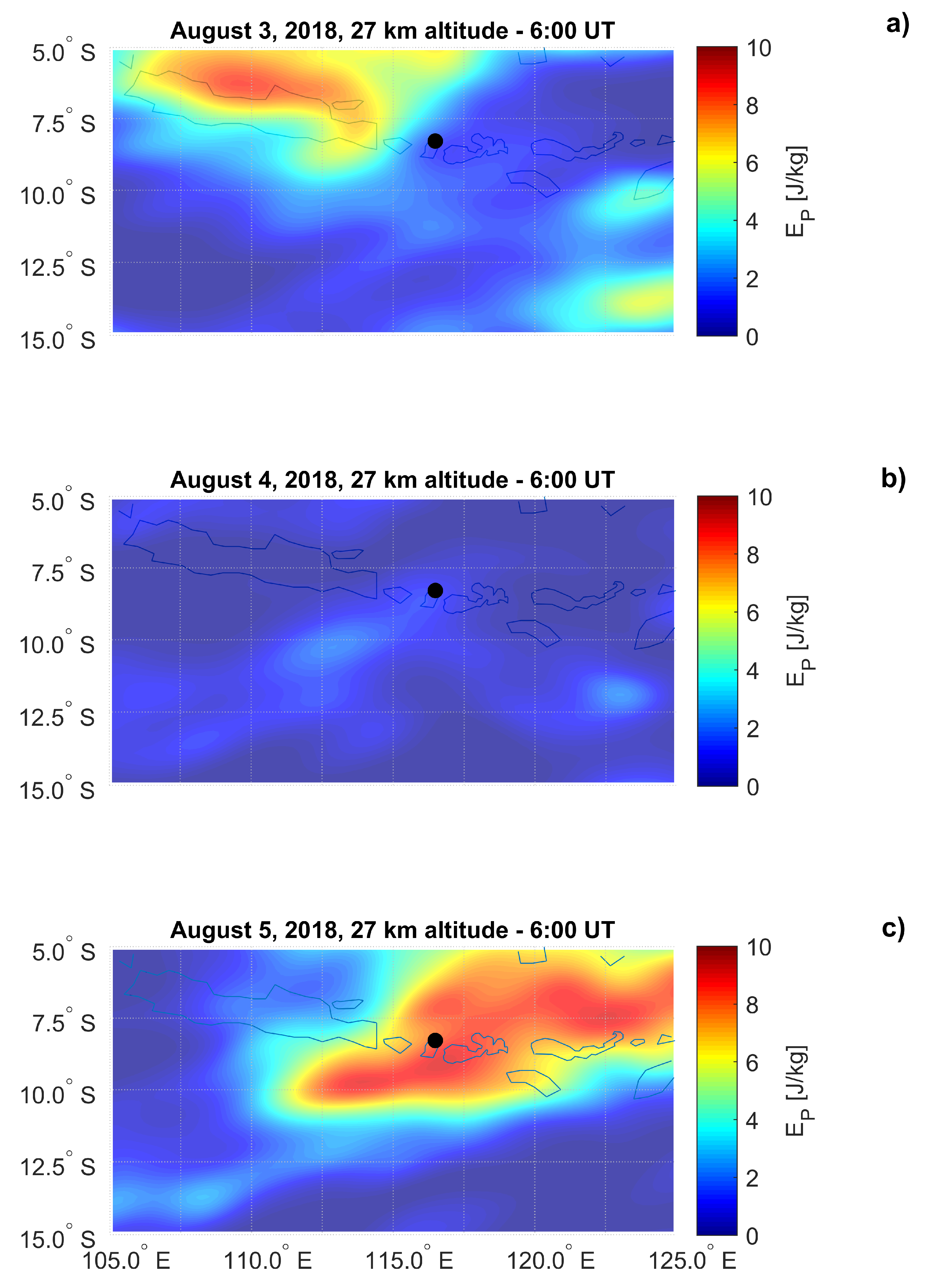
3.1. Acoustic Gravity Waves Observations

Figure 1 shows the $E_P$ calculation for 5 August 2018 at 12:00 UT at the epicenter location. The vertical profiles of the temperature, the background temperature and the temperature deviation are reported in panels (a), (b) and (c), respectively.

Figure 1d,e present the squared term of the $Brunt-V\ddot{a}is\ddot{a}l\ddot{a}$ frequency and the obtained potential energy, respectively. It can be easily seen that the temperature reaches its absolutely maximum at ∼18 km (black dotted line), corresponding to the tropopause [66]. A similar behaviour can be found in both $N^2$ and $E_P$ value [67]. In addition, the potential energy is sometimes additionally enhanced around the stratopause when the temperature changes rapidly with altitude.

In general, AGWs injection is revealed in the temperature deviation (Figure 1c), and its wavelength can be calculated by a full period (if any) variation. In this case, a clear wave can be identified between 5 km and 30 km, whose peaks are at 7.6, 14.1, 23.7 and 27.2 km (red dotted lines), respectively. $E_P$ were maximized at the same altitudes, confirming the injection of AGW. As a consequence, we estimated a ∼7 km vertical wavelength associated with the AGW.

To further check the wave activity around the EE, we evaluated the horizontal distribution of the $E_p$ from 3 to 5 August 2018 (Figure 2). The altitude of these maps was fixed at 27 km, corresponding to the maximum potential energy values between the tropopause (∼17 km) and the stratopause (∼40 km). On 3 August 2018, a clear AGW activity (panel a) is visible at lower latitudes than the EE, caused by a cold front associated with the arrival of a cyclone passing the northern part of Indonesia. On the contrary, 4 August 2018 presents a relatively calm state around the EE (panel b). Interestingly, a strong increase in $E_P$ (panel c) is clearly visible on 5 August 2018 over the EE (black circle), with respect to both of the previous days. The horizontal wavelength of the wave activity (7${}^{\circ }$–11${}^{\circ }$ in longitude) was ∼700–1200 km. Such values are consistent with previous results in Gokhberg and Shalimov [68], Mareev et al. [69] and more recently in Yang et al. [29] who found horizontal AGW wavelength associated to EQ or explosions between 400–1000 km.

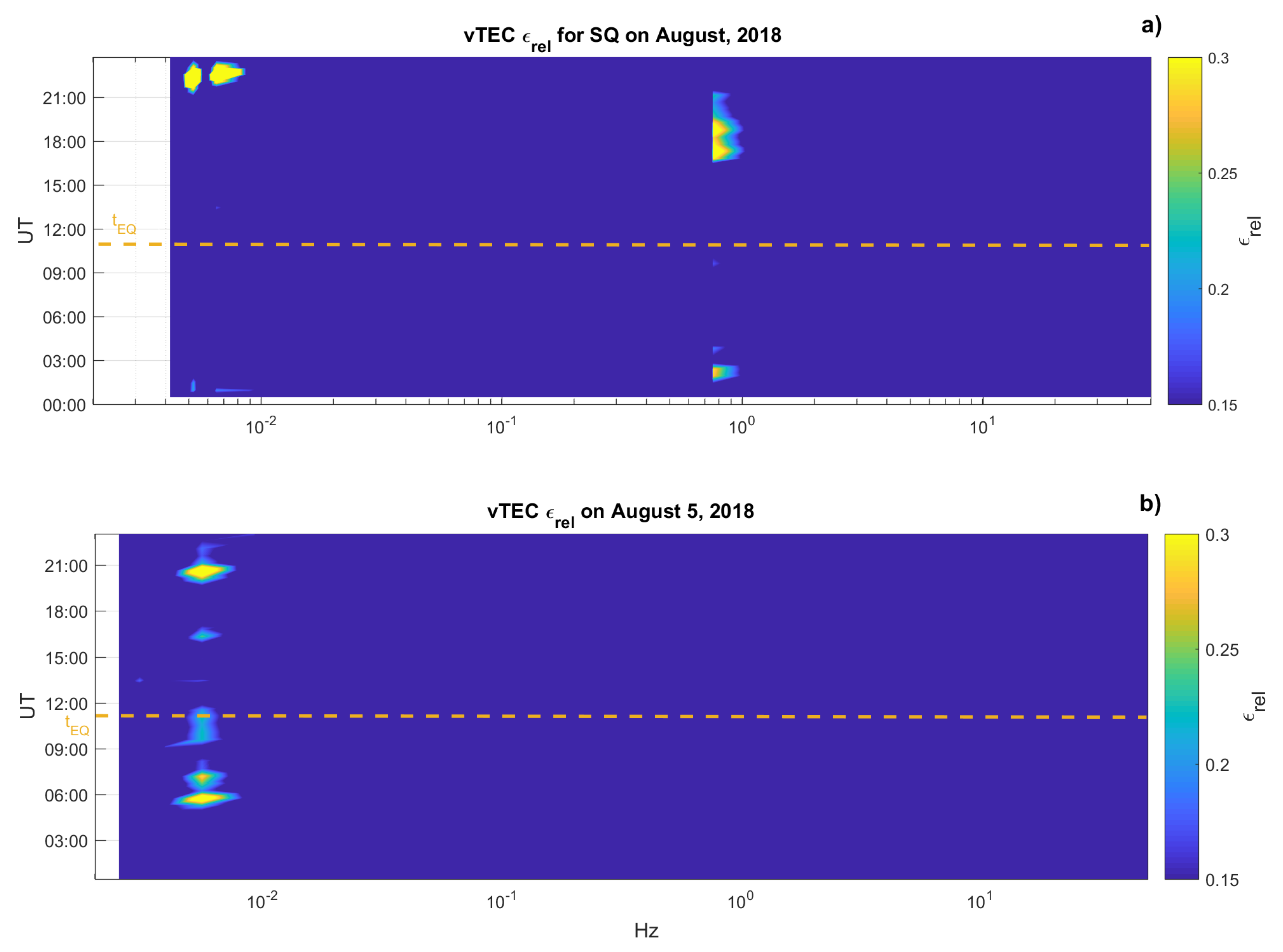
3.2. Vertical Total Electron Content Observations

To identify possible ionospheric anomalies, we determined the variation in vTEC with respect to its background, as follows:

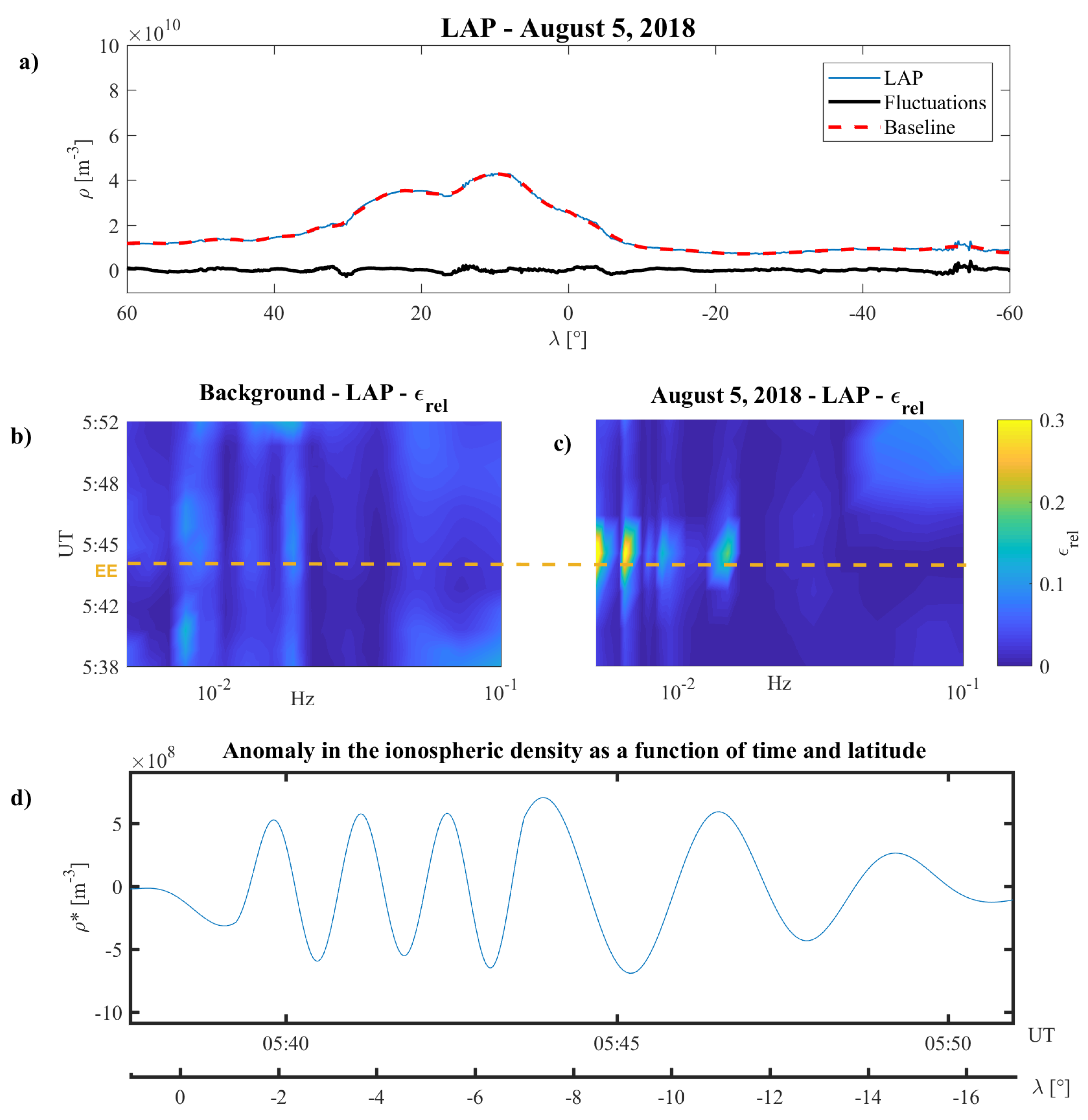
• We identified 10 days of August 2018 characterized by both low solar activity (i.e., −10 nT < Sym-H < 5 nT and $AE<100$ nT, Sym-H and AE being the geomagnetic disturbed time index [70] and Auroral Electrojet index [71], respectively) and low seismic activity (i.e., M < 2, M being the EQ magnitude) in an area of 3${}^{\circ }$× 3${}^{\circ }$ lat × lon around the EE;
• We decomposed the diurnal vTEC observations using the FIF method, which we briefly recalled in Section 2.5. The interested reader can find more details on this algorithm and its pseudo-code in [59,61] FIF code for Matlab is freely available at www.cicone.com);
• We evaluated the 10-day average relative energy spectrogram (${\overline{ϵ}}_{rel}$) after removing the long term trend;
• ${\overline{ϵ}}_{rel}$ is the vTEC background.

Figure 3a shows the evaluated vTEC background over the EQ. Small enhancements in the vTEC values are observed in the local nighttime between 16:00 UT and 20:00 UT (23:00 LT and 03:00 LT). According to Galav et al. [72], this may be due to the pre-reversal enhancement, which is attributed to the variation of the vertical F region drifts at low latitudes.

Figure 3b shows the relative energy for the vTEC on 5 August 2018. It can be easily seen that an anomalous vTEC component ($vTE{C}^{*}$) at $112.3\pm 5$ s switches on at (5:15 ± 0:02) UT and vanishes at (6:35 ± 0:02) UT. Another vTEC component ($vTE{C}^{{}^{\prime \prime }}$), at $97.5\pm 5$ s, switches on at (10:42 ± 0:02) UT vanishing at (11:49± 0:02) UT—i.e., 1 min after the earthquake event.

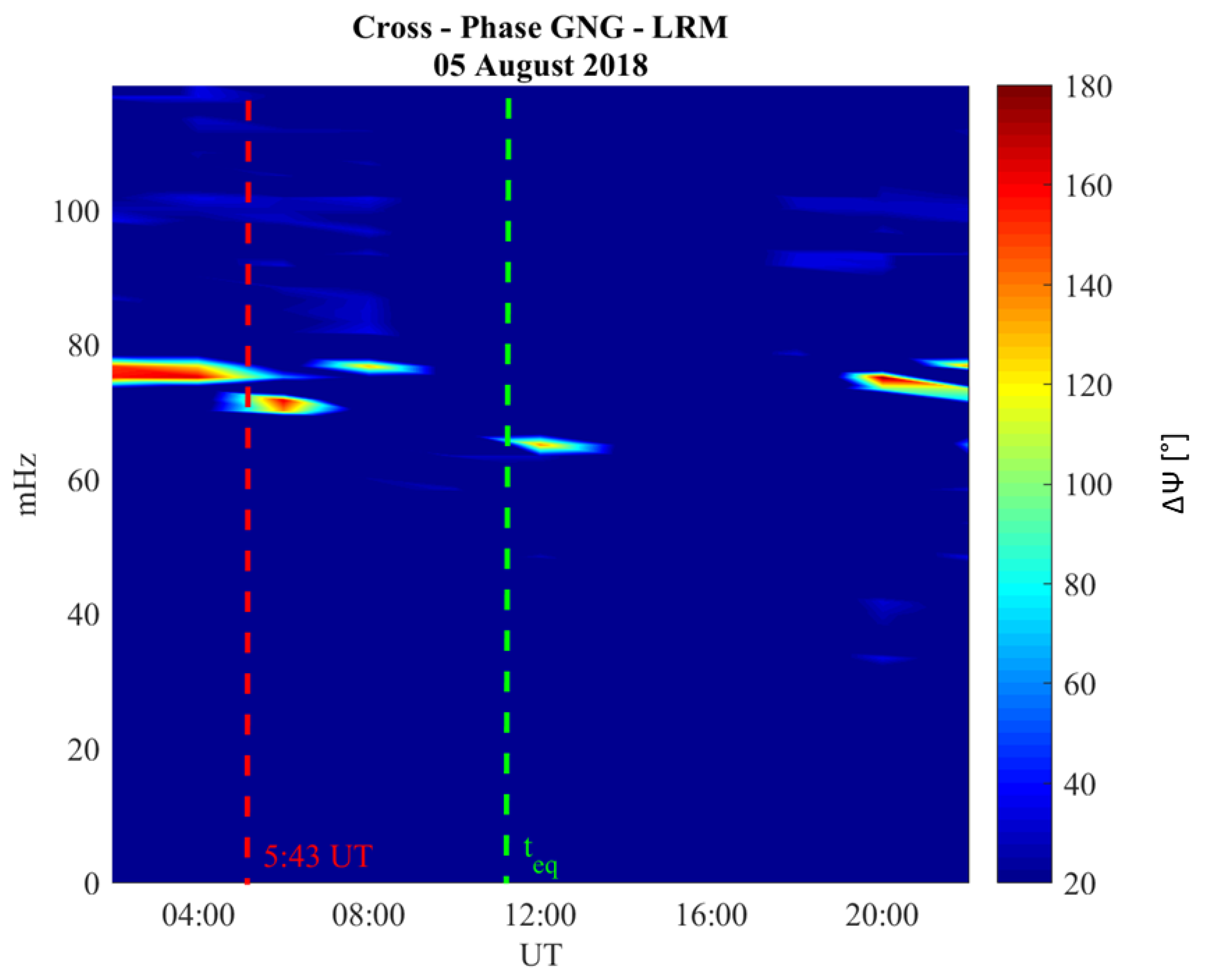
3.3. Magnetospheric Field Line Resonance (FLR) Frequency Observations

Figure 4 shows the evaluation of FLR eigenfrequency through the analysis of the cross-phase spectrum of the H component of the geomagnetic field observed at GNG and LRM. Each spectrum has been evaluated over a 1 h interval and the final spectra have been smoothed both in time and frequency domains (7 frequency bands and 15 temporal bands).

Despite the not-ideal latitudinal distance between the two observatories, we were able to correctly estimate the FLR eigen-frequency behavior ($f^{*}$) throughout the entire day. Indeed, between 01:00 UT and 04:00 UT, a stable maximum of the cross-phase is at $78\pm 2$ mHz, as expected [47]. At 5:43 ± 0:05 UT (red dashed line) there is a clear shift of $f^{*}$ at a lower value ($71\pm 2$ mHz). $f^{*}$ came back to its typical values at 7:36 ± 0:05 UT. Interestingly, in conjunction with the EQ time (green dashed line), there is a more pronounced downward shifting of $f^{*}$ at $62\pm 2$ mHz. As expected, in the local night (i.e., between ∼13:00 UT and ∼20:00 UT), the algorithm was not able to identify the FLR eigen-frequency due to the lower ionospheric conductivity values [46].

4. The Bayan 5 August 2018 Earthquake, Pre-Seismic Observations

This section shows the atmospheric, ionospheric and ground magnetic observations ∼6 h before the EQ occurrence, corresponding to the period of CSES satellite flying over the EE (see Figure S1 in the Supplementary Material).

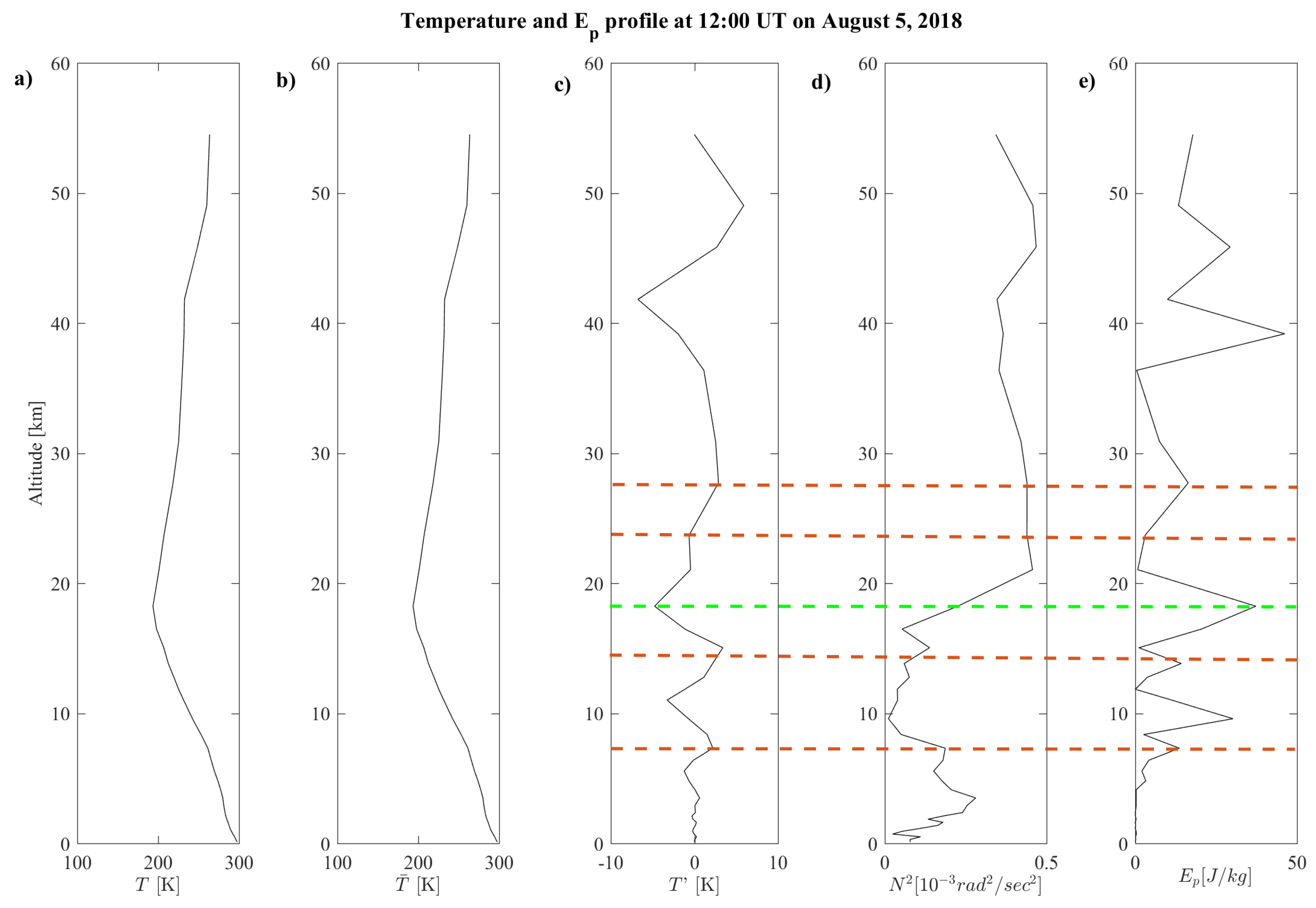
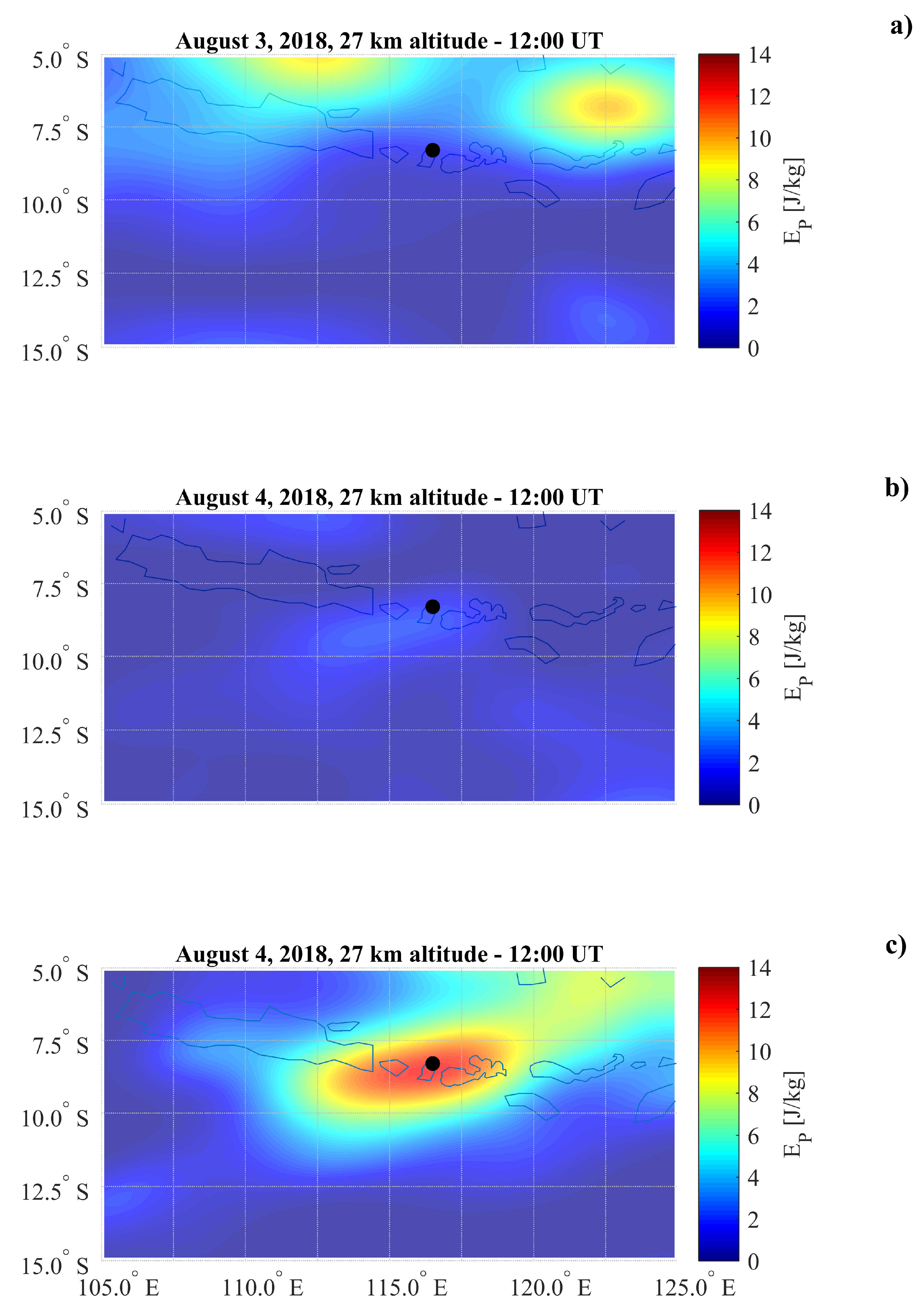
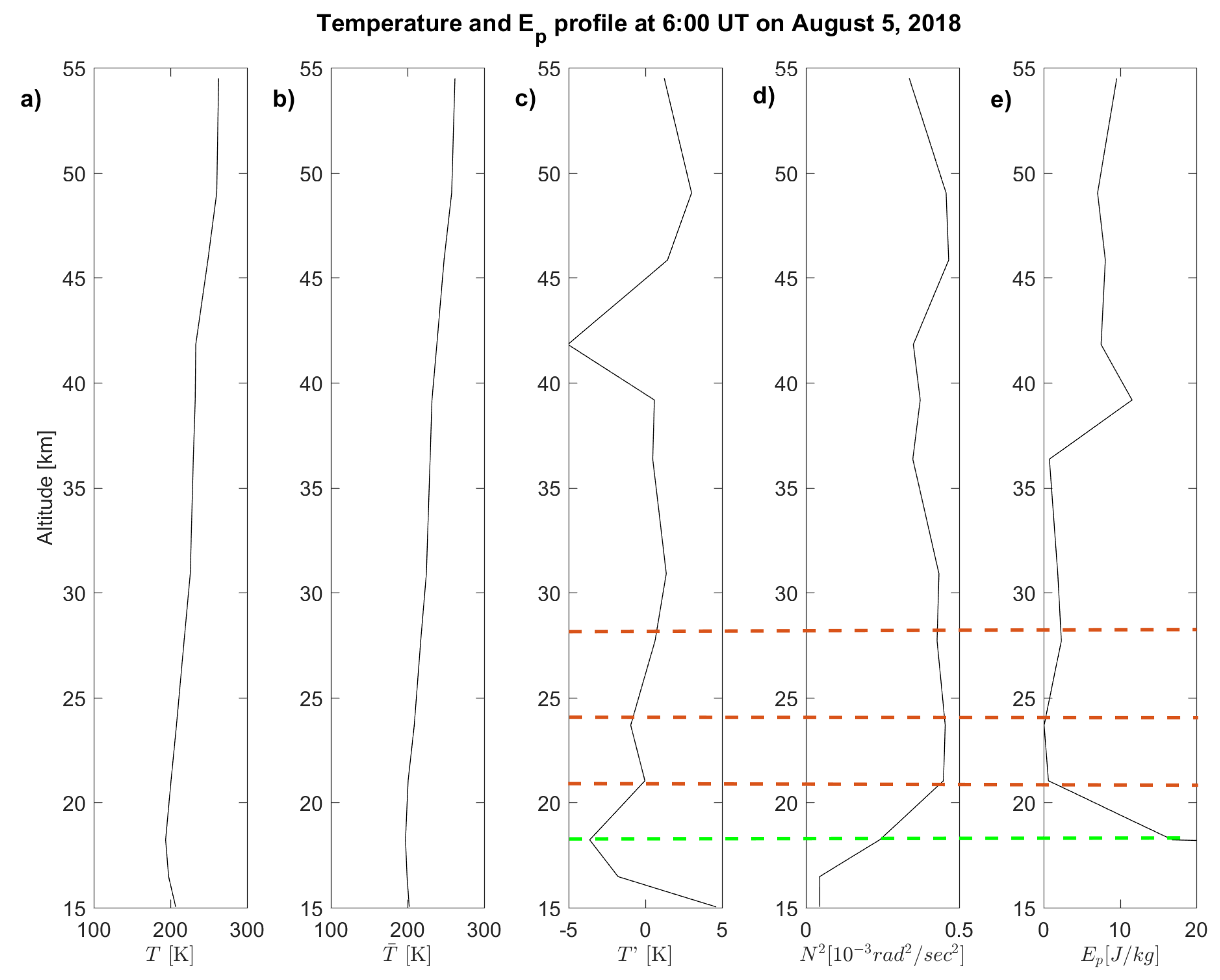
4.1. Atmospheric Temperature Observations

As in the co-seismic analysis section, we evaluated (Figure 5) the $E_P$ values of AGWs at 6:00 UT at the epicenter location. Figure 5a–c show the vertical temperature profile as obtained from ERA5, $\overline{T}$ as obtained by a 2 km moving average and the deviation $T^{\prime }$, as computed by subtracting the background from the original temperature profile, respectively.

Figure 5d,e are the squared term of the $Brunt-V\ddot{a}is\ddot{a}l\ddot{a}$ frequency and the resulted AGW potential energy. Additionally, in this case, as expected [67], we found that the temperature value reached its absolutely maximum at the tropopause (∼17 km). $T^{\prime }$ shows clear waves identified between 21 km and 37 km, whose peaks are at 21.3, 24.1, and 27.3 km, respectively. The maximization of $E_P$ at this altitude confirms the injection of AGW, whose estimated vertical wavelength is ∼3 km.

Additionally, in this case, to confirm the wave activity beyond the EE, we evaluated the horizontal distribution of the $E_p$ from 3 to 5 August 2018 (Figure 6). The altitude of these maps was fixed at 27 km, corresponding to the maximum potential energy values between the tropopause (∼17 km) and the stratopause (∼39 km). Panels (a) and (b) confirm the arrival of a cold front associated to the a cyclone arriving at the northern part of Indonesia on 3 August 2018, and the relative calm state on 4 August 2018. Interestingly, a strong increase in $E_P$ (panel c) is clearly visible on 5 August 2018 over the EE (black circle), with respect to both the previous days. The horizontal wavelength of the wave activity is (∼15${}^{\circ }$ in longitude) ∼1600 km.

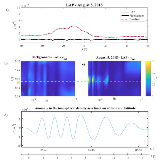
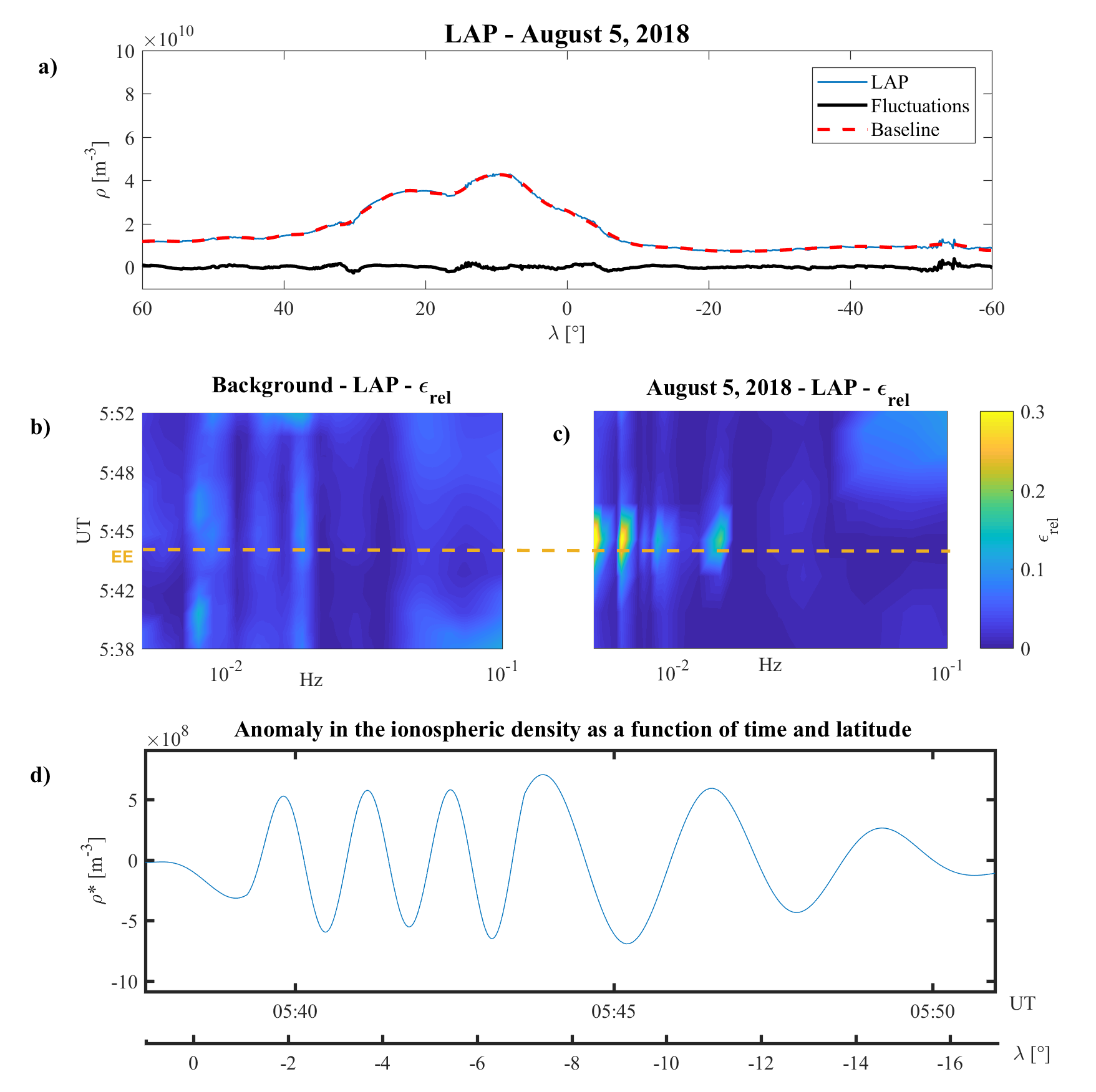
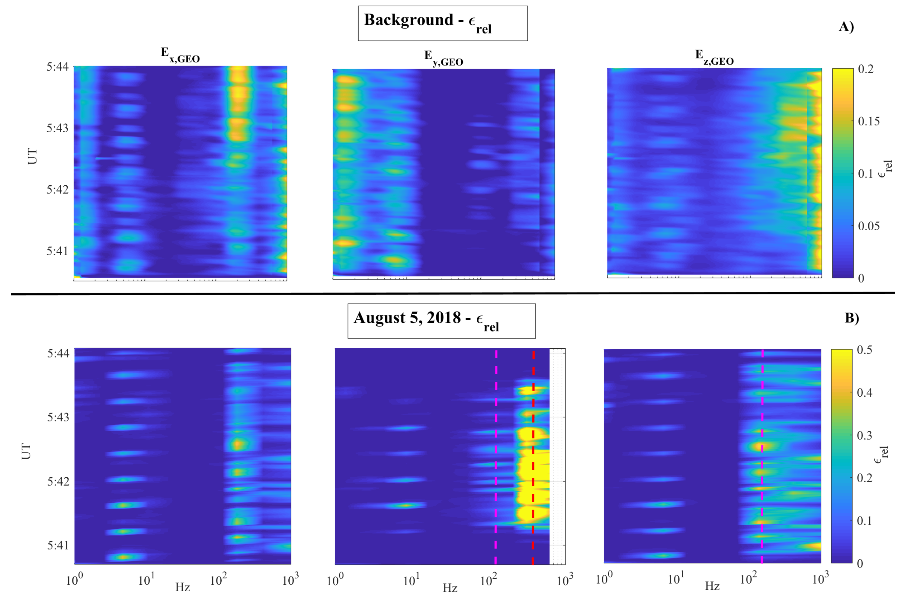
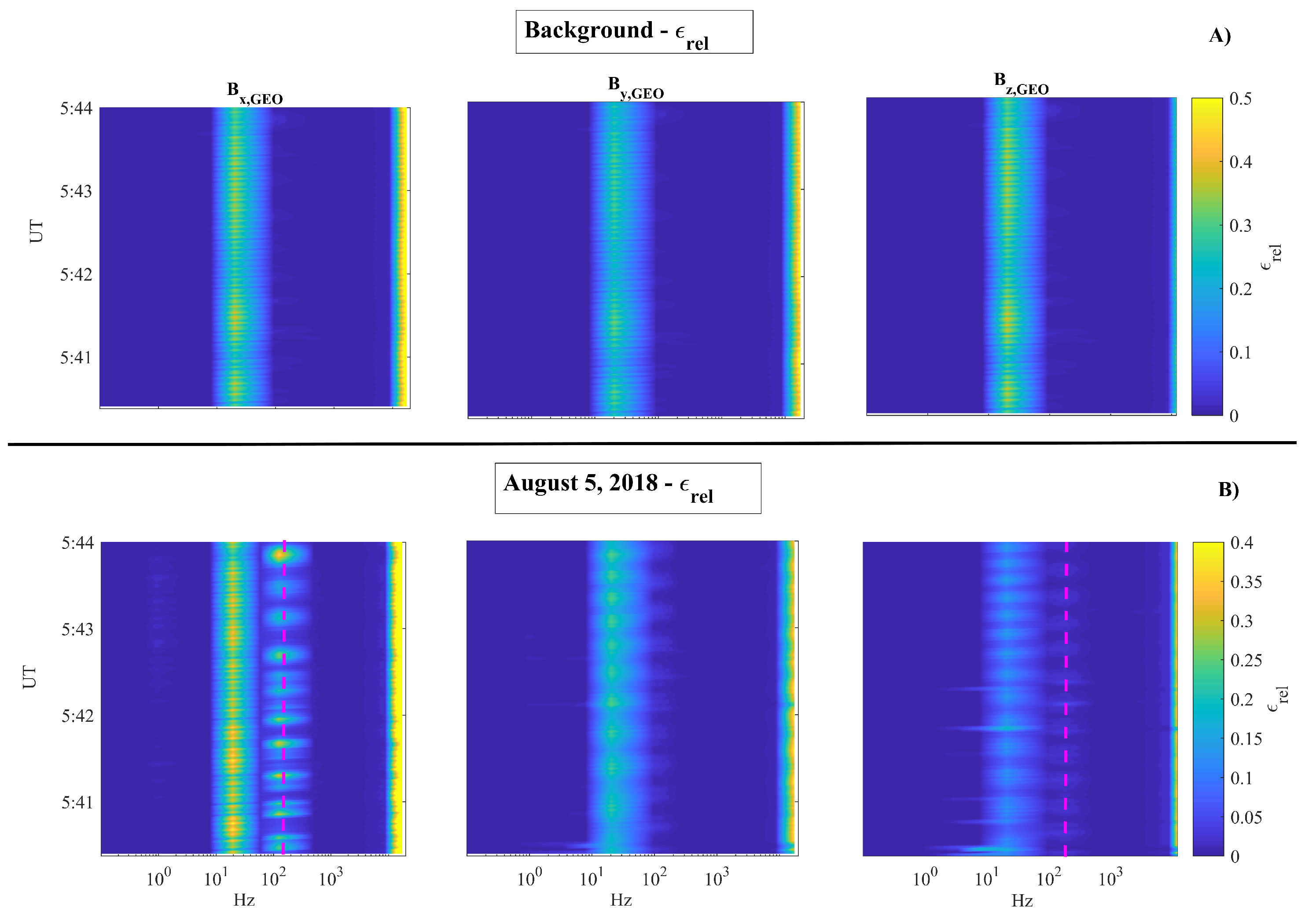
4.2. CSES Satellite Ionospheric Observations

In order to investigate electromagnetic signals possibly associated with 5 August 2018 earthquake, we used CSES satellite electric field, magnetic field and plasma density data. For this purpose, following the approach used in Bertello et al. [73] for DEMETER data, we first decomposed each signal using FIF, than we calculated the relative energy spectrogram (${ϵ}_{rel}$). To detect any EM anomaly possibly related to the EQ, we compared each ${ϵ}_{rel}$ to a background defined in the following way:

• The entire electric and magnetic field dataset is divided into two subsets depending on different seismic conditions: $M_L$ defined for low seismic activity (i.e., $M\le 2$); $M_H$ defined for high seismic activity (i.e., $M>2$);
• $M_L$ and $M_H$ is divided into three groups according to the geomagnetic activity. This procedure made use of Sym-H and AE geomagnetic indices. The three subgroups correspond to low, moderate and high geomagnetic activity, namely: $I_{k,1}$ - Sym-H = [10 nT, −10 nT] and AE < 100 nT; $I_{k,2}$ - Sym-H = [−10 nT, 80 nT] and AE < 200 nT; $I_{k,3}$ - Sym-H $\le -80$ nT and AE ≥ 200 nT;
• A cell $3^{\circ }\times 3^{\circ }$ in latitude–longitude centered over the EE, in which we evaluated the time-frequency average ${\overline{ϵ}}_{rel}$, is selected. The mean operation is applied only if the ratio $R_{ϵ}\left(f\right)=\frac{{ϵ}_{rel}}{{\overline{ϵ}}_{rel}}=1\pm 4\sigma \left(f\right)$, $\sigma \left(f\right)$ being the standard deviation of ${\overline{ϵ}}_{rel}$ evaluated for each frequency scale.
• Each frequency scale showing a $K_{ex}$ almost null and correspondingly a relative maximum in the Shannon entropy (I) was not considered in the evaluation of the relative energy, since it can be represented as a Gaussian fluctuation characterized by high “degree of randomness”—i.e., instrumental noise [58].

We define the evaluated ${\overline{ϵ}}_{rel}$ as the background, since it gives a representation of the magnetospheric and ionospheric electromagnetic activity directly induced by the sun. As a consequence, any distinct signal over $1\pm 4\sigma$ can be reasonably identified as anomalous.

In the case of the Bayan earthquake, when CSES flew over the EE, the solar activity was very low (1 nT < Sym-H < 6 nT) and AE < 100 nT. As a consequence, we evaluated the ${\overline{ϵ}}_{rel}$ relative to $I_{k,1}$ interval. In addition, the background was calculated for both EFD and SCM data, using data from August 2018 to November 2019.

Figure 7A shows the electric field background ${\overline{ϵ}}_{rel,EFD}$ for the geographic North–South ($E_x$, left panel), East–West ($E_y$, middle panel) and vertical ($E_z$, right panel) components. A clear signature of the ionospheric Schumann resonance at ∼7.9 Hz is visible in all components [74]. The peaks detected at a frequency of around 2 Hz are due to the $v_s\times B$ electric field, induced by the motion of the satellite with a velocity $v_s$ into a magnetic field B. The peak around 1 kHz, in both $E_x$ and $E_z$, can be related to the signature of the plasmaspheric hiss [75,76]. Finally, the peak around 270 Hz along $E_x$ is a portion of the whistler mode chorus generated around $L_{shell}=5$ propagating into the plasmasphere [77,78]. Figure 7B shows the relative energy evaluated for 5 August 2018. As expected, the Schumann resonance peak at ∼7.9 Hz is clearly visible in all components. Interestingly, anomalous peaks at ∼180 Hz along $E_y$ and $E_z$ (magenta vertical dashed lines), and at ∼630 Hz along $E_y$ (red vertical dashed lines) can be easily identified with respect to the background.

The results of the same analysis repeated for the magnetic field measurements are presented in Figure 8 along the geographic North–South ($B_x$, left panel), East–West ($B_y$, middle panel) and vertical ($B_z$, right panel) components. Here the ${\overline{ϵ}}_{rel,SCM}$ background (box A) shows the signature of the second Schumann ionospheric resonance at $\sim 20$ Hz. In addition, a peak is clearly visible at 12 kHz, probably related to the lower-hybrid resonance of the ionospheric F2 layer [79]. Figure 8B shows the relative energy of the SCM on 5 August 2018. The second Schumann resonance is clearly visible in all components and an anomalous peak at $\sim 180$ Hz appears along $B_x$ and $B_z$ (magenta vertical dashed lines). Such oscillation has the same frequency and is perpendicular to that detected in the EFD data. As a consequence, it is an electromagnetic wave. The analysis of the Poynting flux (see Figure S3 in the Supplementary Material), confirms that such an electromagnetic wave propagates upward.

Figure 9a shows the CSES LAP data (blue line) for the entire selected semi-orbit (Figure S1 in the Supplementary Material).As expected for solar quiet conditions, the density presents a local maximum around the magnetic equator and greatest variations at high latitudes [80]. In order to find possible low amplitude variations (with respect to the long term trend value) switching on over the EQ cell, we removed the long term trend (red line) and analyzed the plasma density fluctuations (black line) using FIF. Figure 9b,c show the LAP background relative energy evaluated from August 2018 to November 2019 for solar quiet conditions and 5 August 2018 ${ϵ}_{rel}$, respectively. Two anomalous density components switched on between 5:39 ± 00:02 UT and 05:50 ± 00:02 UT characterized by $T_1=67\pm 1$ s and $T_2=111\pm 1$ s peculiar periods.

Figure 9d presents plasma density anomaly ($\rho *$) obtained by the superposition of the two frequency components, $T_1$ and $T_2$. It can be easily seen that the $\rho *$ switches on near the EE, reaching its maximum values at EE and then vanishing.

5. Discussion

The analysis presented in this paper is based on a multi-instrumental observations in relation to the 5 August 2018 Bayan earthquake. We divided the analysis into two parts, relative to the co-seismic and pre-seismic observations, making a direct comparison among atmospheric oscillations, ionospheric plasma and electric field perturbations, and magnetospheric FLR eigenfrequency variations. First of all, atmospheric temperature data confirm the injection, over the EE, of a clear co-seismic AGW characterized by a ∼7 km vertical wavelength. A concomitant (1 min after the EQ occurrence) vTEC perturbation ($vTE{C}^{\prime \prime }$), characterized by a period of ∼97 s, was identified with respect to its background. Finally, a clear decrease in the magnetospheric FLR $f^{*}$ was found ∼2 min after the EQ.

The same analysis was repeated ∼6 h before the earthquake, corresponding to the time of the CSES-01 satellite flying over the EE. Additionally, in this case, at ∼6:00 UT, we detected an AGW characterized by a ∼3 km vertical wavelength. In addition, a vTEC perturbation ($vTEC*$), characterized by a period of $112.3\pm 5$ s, switches on at ∼5:15 UT and vanishes at ∼6:35 UT. The CSES-01 satellite detected an EM wave, at ∼180 Hz, propagating upwards between the ∼5:40 UT and the ∼5:46 UT. Interestingly, the LAP on-board the satellite identifies anomalous density variations, $\rho *$, characterized by ∼70 s and ∼110 s time periods. Lastly, a decrease in the magnetospheric $f^{*}$ was found ∼5:43 UT. The observational scenario presented above can be explained in terms of a Magnetospheric–Ionospheric–Lithospheric Coupling (M.I.L.C.) model, based on three causal steps (see Figure 10):

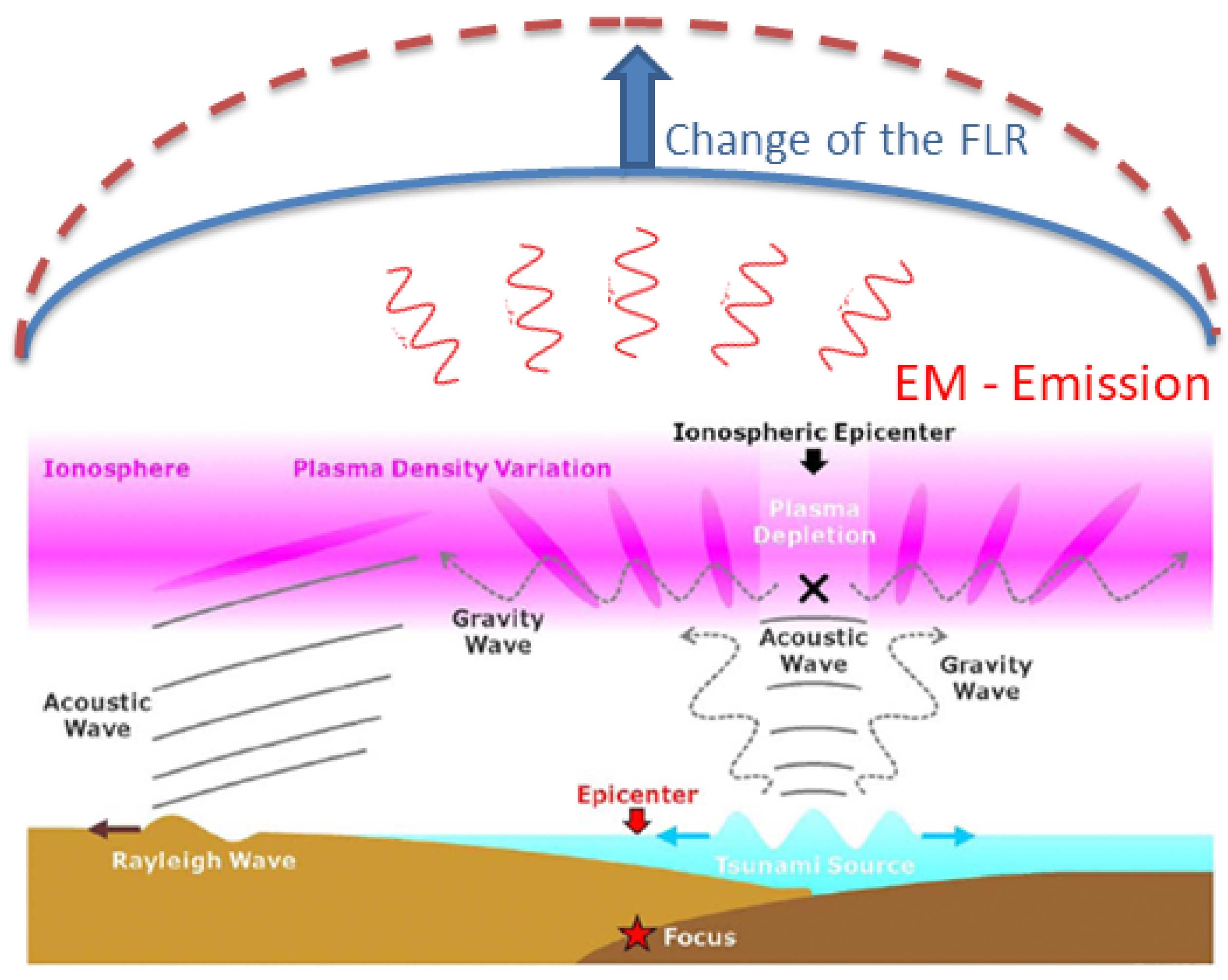
• An AGW is generated around the EE, propagating through the atmosphere;
• The AGW interacts mechanically with the ionosphere, creating a local instability in the plasma distribution through a pressure gradient. Such plasma variation put the ionosphere into a “meta-stable” state, giving rise, in the E-layer, to a local non-stationary electric current. This, in turn, generates an electromagnetic (EM) wave.
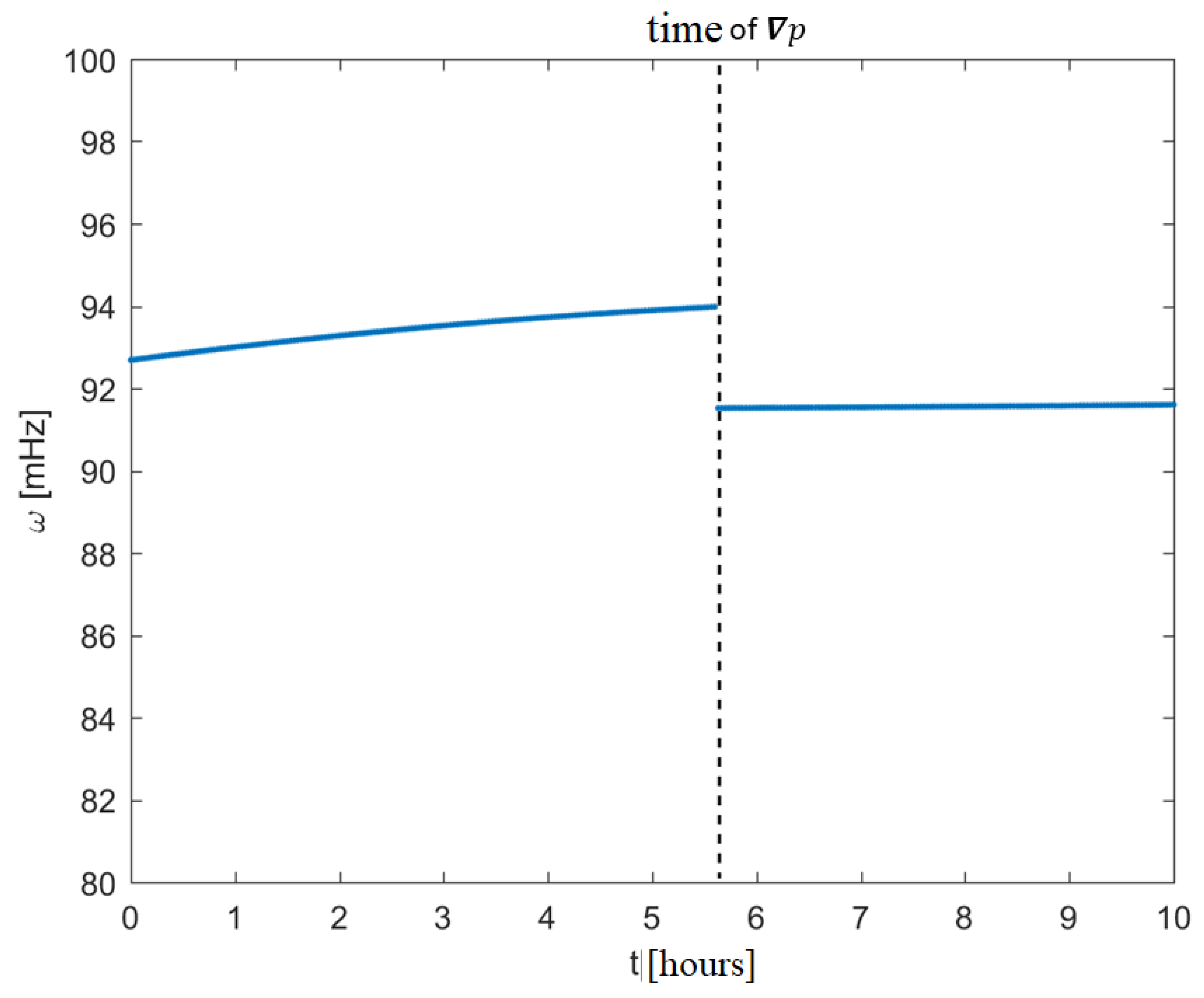
• The interaction of such EM waves with the magnetospheric field causes a change in the eigenfrequency of the field line, whose ionospheric footprint is located over the radial projection of the EE.

This picture is supported by the following mathematical descriptions. Starting from the general equations of compressible, inviscid flow under a gravity field, in absence of external forcing,

$$\left\{\begin{array}{c}\hfill \frac{\partial \rho }{\partial t}+\overrightarrow{\nabla }·\left(\rho \overrightarrow{v}\right)=0\\ \hfill \rho [\frac{\partial \overrightarrow{v}}{\partial t}+(\overrightarrow{v}·\overrightarrow{\nabla })\overrightarrow{v}]+\overrightarrow{\nabla }p=0\\ \hfill \overrightarrow{\nabla }{p}_0={\rho }_0\overrightarrow{g}\\ \hfill {\rho }_0{c}_s^2=\gamma p_0\end{array}\right.$$

(6)

where $\rho$, p, v are the atmospheric density, pressure and velocity, $c_s$ is the sound speed and $\gamma$ is the adiabatic index, we can easily evaluate the exact expression of an AGW propagating in a stratified non-isothermal atmosphere in terms of unsteady, non-uniform pressure perturbation $p^{\prime }$ related by an adiabatic condition in a convected frame [81].

$$\begin{array}{c}\hfill \frac{{\partial }^{2}p}{\partial t^2}-c_s^2{\nabla }^{2}p+A·p=0,\end{array}$$

(7)

where $A=\gamma g^2/c_s$. The solution of Equation (7) is a mechanical wave (Lamb wave) [82,83]. As expected, the dispersion relation of such an excited waveform mainly depends of the phase speed of the surface waves of earthquake $v_s$. The intensity of the perturbation depends on the height of the atmosphere where it was excited, and on the characteristic of the earthquake, namely the phase speed $v_s$, the frequency of surface waves ${\omega }_s$, the Peak Ground Acceleration and the Strong Motion Duration of the earthquake. In this case, the earthquake had a magnitude of $Mw=6.9$ and, according to the seismic surface waves dispersion relation, registered a frequency on the ground of ${\omega }_s\simeq 0.58$ Hz (USGS data catalog: https://earthquake.usgs.gov/earthquakes/eventpage/us1000g3ub/executive), thus corresponding to a phase speed of $c_s\simeq 4.5$ km/s. The measured Peak Ground Acceleration was ≃0.8 g, and the Strong Motion Duration was of ≃20 s. According to our model, this induces an intense atmospheric perturbation up to an length of about $H\simeq 10$ km, and the waveform was excited with frequencies in the range $0.5\le \omega \le 2$ Hz and wavevectors $500\le k\le 3000$ m. This range values agrees with the AGWs detected using ERA-5 data (see Figure 1 and Figure 5). In addition, such perturbation was able to propagate, at the sound speed, in the vertical direction [84] and reach the ionosphere.

Putting the $\overrightarrow{\nabla }{p}^{\prime }$ as the external forcing into the Magneto–Hydro–Dynamic equation of a uniform ionosphere, located at 100 km with respect to the Earth’s surface and whose plasma density decrease as $z^{-2}$ with the altitude z, a ionospheric plasma density variation is induced [85]. Indeed, if the Magneto–Hydro–Dynamic system is solved for the perturbation of the electric field $\overrightarrow{E}$, an EM wave, in the frequency range between 10–700 Hz, is generated, propagating from the topside ionosphere. Additionally, in this case, such prevision is in agreement with our observations (see Figure 7 and Figure 8). At low latitudes (i.e., $0^{\circ }\le \lambda \le {30}^{\circ }$), the concurring contribution of the EM wave energy and of the plasma density variation produces a change in the local FLR eigen-frequency. In fact, the resonance frequencies of a geomagnetic field line, with both ends fixed in the ionosphere depend on the field line length, and on the magnetic field intensity and plasma mass density $\rho$ along the field line [86,87,88,89,90,91,92]. A crude estimation of an FLR eigen-frequency (f) is given by the time of flight approximation [93] as:

$$\begin{array}{c}\hfill \frac{1}{f}=2{\int }_s\frac{ds}{V_A}\\ \hfill V_A=\frac{B\left(s\right)}{\sqrt{{\mu }_0\rho \left(r\right)}}\end{array}$$

where $V_A$ is the Alfvén speed along the field line, $B\left(s\right)$ is the magnetospheric field along the field line, and $\rho \left(r\right)$ is the density at geocentric distance r. As a consequence, a change in the field line length and/or the $V_A$, caused a variation in the FLR frequency [94]. The result of the modeled $f^{*}$ variation of a field line footprinted at $\lambda ={10}^{\circ }$, under the assumption of a pure dipolar Earth’s magnetic field, associated with a pressure gradient driven by an earthquake of Mw = 6.9, is reported in Figure 11. A clear decrease in $f^{*}$ is visible in coincidence to the pressure gradient ($\overrightarrow{\nabla }p$) driven by the AGW injected by the earthquake. A similar situation is clearly visible in Figure 4. The complete mathematical description of the model will be presented in the second paper.

Despite the fact that the event described above fits very well with the model presented here, many issues are still opened and need a careful inspection.

First of all, if the detection of an AGW propagating through the atmosphere is quite simple (see Figure 1), its direct association to an EQ phenomena is not trivial. It is well known that the generation of AGWs during an EQ can be due to different reasons, such as unstable thermal anomalies that originate from the outflow of greenhouse gases into the atmosphere in fracture regions of the Earth’s crust, the oscillation of the Earth’s crust having a block-like structure, and so on. Such anomalies can be found in the atmospheric temperature, pressure and/or conductivity [95]. In any case, earthquakes are not the one and the only driver of gravity waves propagating through the atmosphere. In fact, AGW are generally induced by weather systems, by synoptic-scale atmospheric systems and circulations, and similar processes [28,96,97], and can affect temperature and wind fields in the higher atmosphere. At middle and low latitudes (i.e., where the EQs are more recurrent), AGWs in general are meteorologically excited by convective activities around the cold fronts [28]. In our case, following the approach of Yang et al. [29], in order to be sure that the AGW detected either ∼6 h before and at the moment of 5 August 2018 EQ occurrence, we tried to exclude all the other possibilities. For this purpose we examined the weather reports (https://www.accuweather.com/) for 5 August 2018 and we found a tropical cyclone passing the Indonesia around the 12:00 UT, but the cold fronts associated with such a cyclone were essentially located in northern Indonesia, over the Brunei region (i.e., far from the EE). In addition, the weather data over the Bayan zone showed that thunderstorms occurred on 7 and 12 August. So, we are confident that both the AGWs detected at 6:00 UT and at 12:00 UT can be associated to the seismic activity.

Second, the correct discrimination between ionospheric plasma density variations induced by internal and external origin sources is crucial. In general, both vTEC and plasma density irregularities are directly driven by the solar activity—e.g., in [98]. In the present case, the visual inspection of both the solar wind (SW) parameters and the geomagnetic indices (i.e., Sym-H and AE) confirms that 5 August 2018 was a super-solar quiet day [63,99]. In fact, solar wind parameters (see Figure S2 in Supplementary Material) confirms the absence of any structure coming from the sun. On the other hand, as shown in the section above, the values of Sym-H (−5 nT < Sym-H < 6 nT) and AE (AE<100 nT), confirms the low geomagnetic activity either at low and at high latitudes. As a consequence, we can establish that both vTEC* and vTEC” variations are not driven by the sun and can be reasonably associated with the earthquake activity. For the same reason, we can infer that both the variation in $f^{*}$ and the EM activity detected by the CSES-01 satellite are linked to the seismic activity through the process described in the presented model.

Last but not least, while it is easy to connect the AGWs observed around 12:00 to the earthquake, the possible source exciting the AGW detected around 06:00 UT needs an accurate discussion. In our opinion, the possible explanation of pre-earthquake AGW can be either due to the very high-levels of seismic activity of the Lombok 2018 sequence characterized by four strong Mw $>6.3$ within 1 month, or to the outflow of charged gases (e.g., radon) by the Earth’s surface [9,29]. Both hypotheses are reliable in the present case. In fact, on the one hand surface deformations generating variations in atmospheric temperature (hence AGW formation) are very common during high seismic activity—e.g., in [4]. Such a possibility could be well represented by the M.I.L.C. model since the physical mechanism beyond is quite similar to the co-seismic situation [6]. On the other hand, the lack of local surface gas emission data (radon or charged gases in general) do not allow us to exclude the second hypothesis. In any case, this kind of discharge is, in general, coupled with sub-ionospheric very low frequency electromagnetic emission [29]. In the present case, the visual inspection of the very low frequency channel in the EFD on-board CSES did not show any possible anomalous signal, while, as shown in Figure 7 and Figure 8, an electromagnetic signal in the extreme low frequency band was clearly detected.

6. Conclusions

The correct identification of atmospheric, ionospheric and/or magnetospheric perturbations possibly connected to seismic activity has become a research focus in the last few decades. Indeed, thanks to the large increase in ground sounding stations and satellites, many observations of ionospheric and/or atmospheric disturbances, related to seismic activity, have been reported. This paper presents a multi-instrumental analysis of the 5 August 2018 Lombok (Bayan) EQ. There is supported evidence that during the EQ there was an activation of the lithosphere–atmosphere–ionosphere–magnetosphere chain, which, starting from the fault break, generates an AGW able to mechanically perturb the ionospheric plasma density, driving the generation of both EM waves and magnetospheric FLR eigen-frequency variation. The EQ scenario presented here represents an optimal case event to be studied and understood since it happened during both super solar quiet and fair weather conditions. We explained such observations through a new developed analytical “M.I.L.C.” model, whose complete analytical description and details will be provided in a forthcoming paper (i.e., paper 2). Interestingly, the observations of the CSES-01 satellite flying over the EE around 6 h before the EQ, confirms both the presence of EM wave activity, coming from the lower ionosphere, and plasma density variation ($\rho *$) consistent with the vTEC anomaly detected (vTEC*). Finally, we have to stress that the simultaneous availability of both ground and LEO satellite data represented a peculiar feature of the analyzed EQ event which allows us to test and validate the robustness of the presented M.I.L.C. model.

References

1. Hayakawa, M. Earthquake Prediction with Radio Techniques; John Wiley: Singapore, 2015. [Google Scholar] [CrossRef]
2. Molchanov, O.A.; Hayakawa, M. Subionospheric VLF signal perturbations possibly related to earthquakes. J. Geophys. Res. 1998, 103, 17489–17504. [Google Scholar] [CrossRef]
3. Pulinets, S.A.; Boyarchuk, K. Ionospheric Precursors of Earthquakes; Springer: Berlin/Heidelberg, Germany, 2004. [Google Scholar]
4. Hayakawa, M.; Kasahara, Y.; Nakamura, T.; Muto, F.; Horie, T.; Maekawa, S.; Hobara, Y.; Rozhnoi, A.A.; Solovieva, M.; Molchanov, O.A. A statistical study on the correlation between lower ionospheric perturbations as seen by subionospheric VLF/LF propagation and earthquakes. J. Geophys. Res. 2010, 115, A09305. [Google Scholar] [CrossRef]
5. Liu, J.Y. Earthquake precursors observed in the ionospheric F-region. In Electromagnetic Phenomena Associated with Earthquakes; Hayakawa, M., Ed.; Transworld Research Network: Trivandrum, India, 2009; pp. 187–204. [Google Scholar]
6. Pulinets, S.A.; Ouzounov, D.P. Lithosphere–atmosphere–ionosphere coupling (LAIC) model—An unified concept for earthquake precursors validation. J. Asian Earth Sci. 2011, 41, 371–382. [Google Scholar] [CrossRef]
7. Pulinets, S.A.; Ouzounov, D.P.; Karelin, A.V.; Davidenko, D.V. Physical bases of the generation of short-term earthquake precursors: A complex model of ionization-induced geophysical processes in the lithosphere-atmosphere-ionosphere-magnetosphere system. Geomagn. Aeron. 2015, 55, 521–538. [Google Scholar] [CrossRef]
8. Sorokin, V.M.; Yaschenko, A.K.; Hayakawa, M. Formation mechanism of the lower-ionospheric disturbances by the atmosphere electric current over a seismic region. J. Atmos. Sol.-Terr. Phys. 2006, 68, 1260–1268. [Google Scholar] [CrossRef]
9. Hayakawa, M.; Kasahara, Y.; Nakamura, T.; Hobara, Y.; Rozhnoi, A.; Solovieva, M.; Molchanov, O.; Korepanov, V. Atmospheric gravity waves as a possible candidate for seismo-ionospheric perturbation. J. Atmos. Electr. 2011, 31, 129–140. [Google Scholar] [CrossRef] [Green Version]
10. Miyaki, K.; Hayakawa, M.; Molchanov, O.A. The role of gravity waves in the lithosphere-ionosphere coupling, as revealed from the subionospheric LF propagation data. In Seismo Electromagnetics: Lithosphere-Atmosphere- Ionosphere Coupling; Hayakawa, M., Molchanov, O.A., Eds.; TERRAPUB: Tokyo, Japan, 2002; pp. 229–232. [Google Scholar]
11. Molchanov, O.A.; Hayakawa, M.; Miyaki, K. VLF/LF sounding of the lower ionosphere to study the role of atmospheric oscillations in the lithosphere-ionosphere coupling. Adv. Polar Upper Atmos. Res. 2001, 15, 146–158. [Google Scholar]
12. Muto, F.; Kasahara, Y.; Hobara, Y.; Hayakawa, M.; Rozhnoi, A.; Solovieva, M.; Molchanov, O.A. Further study on the role of atmospheric gravity waves on the seismo-ionospheric perturbations as detected by subionospheric VLF/LF propagation. Nat. Hazards Earth Syst. Sci. 2009, 9, 1111–1118. [Google Scholar] [CrossRef] [Green Version]
13. Freund, F. Time-resolved study of charge generation and propagation in igneous rocks. J. Geophys. Res. 2000, 105, 11001–11019. [Google Scholar] [CrossRef] [Green Version]
14. Freund, F. Pre-earthquake signals: Underlying physical processes. J. Asian Earth Sci. 2011, 41, 383–400. [Google Scholar] [CrossRef]
15. Liperovsky, V.A.; Pokhotelov, O.A.; Meister, C.-V.; Liperovskaya, E.V. Physical models of coupling in the lithosphere-atmosphere-ionosphere system before earthquakes. Geomagn. Aeron. 2008, 48, 795–806. [Google Scholar] [CrossRef]
16. Oyama, K.-I.; Devi, M.; Ryu, K.; Chen, C.H.; Liu, J.Y.; Liu, H.; Bankov, L.; Kodama, T. Modifications of the ionosphere prior to large earthquakes: Report from the ionospheric precursor study group. Geosci. Lett. 2016, 3, 6. [Google Scholar] [CrossRef] [Green Version]
17. Hayakawa, M.; Molchanov, O.A.; Ondoh, T.; Kawai, E. The precursory signature effect of the Kobe earthquake on VLF subionospheric signals. J. Commun. Res. Lab. 1996, 43, 169–180. [Google Scholar] [CrossRef]
18. Korepanov, V.; Hayakawa, M.; Yampolski, Y.; Lizunov, G. AGW as a seismo-ionospheric coupling responsible agent. Phys. Chem. Earth Parts A B C 2009, 34, 485–495. [Google Scholar] [CrossRef]
19. Nakamura, T.; Korepanov, V.; Kasahara, Y.; Hobara, Y.; Hayakawa, M. An evidence on the lithosphere-ionosphere coupling in terms of atmospheric gravity waves on the basis of a combined analysis of surface pressure, ionospheric perturbations and ground-based ULF variations. J. Atmos. Electr. 2013, 33, 53–68. [Google Scholar] [CrossRef] [Green Version]
20. Endo, T.; Kasahara, Y.; Hobara, Y.; Sue, T.; Hayakawa, M. A note on the correlation of seismo-ionospheric perturbations with ground motions as deduced from F-net seismic observations. J. Atmos. Electr. 2013, 33, 69–76. [Google Scholar] [CrossRef] [Green Version]
21. Hayakawa, M.; Hobara, Y.; Yasuda, Y.; Yamaguchi, H.; Ohta, K.; Izutsu, J.; Nakamura, T. Possible precursor to the March 11, 2011, Japan earthquake: Ionospheric perturbations as seen by subionospheric very low frequency/low frequency propagation. Ann. Geophys. 2012, 55, 95–99. [Google Scholar] [CrossRef]
22. Hayakawa, M.; Hobara, Y.; Rozhnoi, A.; Solovieva, M.; Ohta, K.; Izutsu, J.; Nakamura, T.; Kasahara, Y. The ionospheric precursor to the 2011 March 11 earthquake based upon observations obtained from the Japan-Pacific subionospheric VLF/LF network. Terr. Atmos. Ocean. Sci. 2013, 24, 393–408. [Google Scholar] [CrossRef] [Green Version]
23. Hayakawa, M.; Rozhnoi, A.; Solovieva, M.; Hobara, Y.; Ohta, K.; Schekotov, A.; Fedorov, E. The lower ionospheric perturbation as a precursor to the 11 March 2011 Japan earthquake. Geomatics. Nat. Hazards Risk 2013, 4, 275–287. [Google Scholar] [CrossRef] [Green Version]
24. Kamiyama, M.; Sugito, M.; Kuse, M.; Schekotov, A.; Hayakawa, M. On the precursors to the 2011 Tohoku earthquake: Crustal movements and electromagnetic signatures. Geomat. Nat. Hazards Risk 2014, 7, 471–492. [Google Scholar] [CrossRef] [Green Version]
25. Hennermann, K. ERA5 Data Documentation. In Copernicus Knowledge Base. 2017. Available online: https://confluence.ecmwf.int/display/CKB/ERA5+data+documentation (accessed on 19 October 2017).
26. De la Torre, A.; Alexander, P.; Giraldez, A. The kinetic to potential energy ratio and spectral separability from high-resolution balloon soundings near the Andes Mountains. Geophys. Res. Lett. 1999, 26, 1413–1416. [Google Scholar] [CrossRef]
27. VanZandt, T.E. A model for gravity wave spectra observed by Doppler sounding systems. Radio Sci. 1985, 20, 1323–1330. [Google Scholar] [CrossRef] [Green Version]
28. Yang, S.-S.; Pan, C.J.; Das, U.; Lai, H.C. Analysis of synoptic scale controlling factors in the distribution of gravity wave potential energy. J. Atmos. Sol. Terr. Phys. 2015, 135, 126–135. [Google Scholar] [CrossRef]
29. Yang, S.-S.; Asano, T.; Hayakawa, M. Abnormal gravity wave activity in the stratosphere prior to the 2016 Kumamoto earthquakes. J. Geophys. Res. Space Phys. 2019, 124. [Google Scholar] [CrossRef]
30. Mannucci, A.J.; Wilson, B.D.; Yuan, D.N.; Ho, C.H.; Lindqwister, U.J.; Runge, T.F. A global mapping technique for GPS-derived ionospheric total electron content measurements. Radio Sci. 1998, 33, 565. [Google Scholar] [CrossRef]
31. Shen, X.H.; Zhang, X.M.; Yuan, S.G.; Wang, L.W.; Cao, J.B.; Huang, J.P.; Zhu, X.H.; Piergiorgio, P.; Dai, J.P. The state-of-the-art of the China Seismo-Electromagnetic Satellite mission. Sci. China Technol. Sci. 2018, 61, 634–642. [Google Scholar] [CrossRef]
32. Zhou, B.; Yang, Y.Y.; Zhang, Y.T.; Gou, X.C.; Cheng, B.J.; Wang, J.D.; Li, L. Magnetic field data processing methods of the China Seismo-Electromagnetic Satellite. Earth Planet. Phys. 2018, 2, 455–461. [Google Scholar] [CrossRef]
33. Wang, Q.; Huang, J.; Zhang, X.; Shen, X.; Yuan, S.; Zeng, L.; Cao, J. China Seismo-Electromagnetic Satellite search coil magnetometer data and initial results. Earth Planet. Phys. 2018, 2, 462–468. [Google Scholar] [CrossRef]
34. Huang, J.P.; Lei, J.G.; Li, S.X.; Zeren, Z.M.; Li, C.; Zhu, X.H.; Yu, W.H. The Electric Field Detector (EFD) onboard the ZH-1 satellite and first observational results. Earth Planet. Phys. 2018, 2, 469–478. [Google Scholar] [CrossRef]
35. Yan, R.; Guan, Y.B.; Shen, X.H.; Huang, J.P.; Zhang, X.M.; Liu, C.; Liu, D.P. The Langmuir Probe onboard CSES: Data inversion analysis method and first results. Earth Planet. Phys. 2018, 2, 479–488. [Google Scholar] [CrossRef]
36. Liu, C.; Guan, Y.; Zheng, X.; Zhang, A.; Piero, D.; Sun, Y. The technology of space plasma in-situ measurement on the china seismo-electromagnetic satellite. Sci. China Technol. Sci. 2019, 62, 829–838. [Google Scholar] [CrossRef]
37. Li, X.; Xu, Y.B.; An, Z.H.; Liang, X.H.; Wang, P.; Zhao, X.Y.; Nan, Y.F. The high-energy particle package on-board CSES. Radiat. Detect. Technol. Methods 2019, 669–677. [Google Scholar] [CrossRef]
38. Picozza, P.; Battiston, R.; Ambrosi, G.; Bartocci, S.; Basara, L.; Burger, W.J.; Campana, D.; Carfora, L.; Casolino, M.; Castellini, G.; et al. Scientific Goals and In-orbit Performance of the High-energy Particle Detector on Board. Astrophys. J. Suppl. Ser. 2019, 243. [Google Scholar] [CrossRef]
39. Lin, J.; Shen, X.H.; Hu, L.C.; Wang, L.W.; Zhu, F.Y. CSES GNSS ionospheric inversion technique, validation and error analysis. Sci. China Technol. Sci. 2018, 61, 669–677. [Google Scholar] [CrossRef]
40. Chen, L.; Ou, M.; Yuan, Y.P.; Sun, F.; Yu, X.; Zhen, W.M. Preliminary observation results of the Coherent Beacon System onboard the China Seismo-Electromagnetic Satellite-1. Earth Planet. Phys. 2018, 2, 505–514. [Google Scholar] [CrossRef]
41. Baransky, L.N.; Borovkov, J.E.; Gokhberg, M.B.; Krylov, S.M.; Troitskaya, V.A. High resolutionm ethodo f direct measuremenot f the magneticf ield lines’ eigenfrequencies. Planet. Space Sci. 1985, 33, 1369. [Google Scholar] [CrossRef]
42. Piersanti, M.; Alberti, T.; Bemporad, A.; Berrilli, F.; Bruno, R.; Capparelli, V.; Carbone, V.; Cesaroni, C.; Consolini, G.; Cristaldi, A.; et al. Comprehensive analysis of the geoeffective solar event of 21 June 2015: Effects on the magnetosphere, plasmasphere, and ionosphere systems. Sol. Phys. 2017, 292, 169. [Google Scholar] [CrossRef]
43. Vellante, M.; Piersanti, M.; Pietropaolo, E. Comparison of equatorial plasma mass densities deduced from field line resonances observed at ground for dipole and IGRF models. J. Geophys. Res. Space Phys. 2014, 119. [Google Scholar] [CrossRef]
44. Waters, C.L.; Menk, F.W.; Fraser, B.J. The resonance structure of low latitude Pc3 geomagnetic pulsations. Geophys. Res. Lett. 1991, 18, 2293. [Google Scholar] [CrossRef] [Green Version]
45. Menk, F.W.; Mann, I.R.; Smith, A.J.; Waters, C.L.; Clilverd, M.A.; Milling, D.K. Monitoring the plasmapause using geomagnetic field line resonances. J. Geophys. Res. 2004, 109, A04216. [Google Scholar] [CrossRef] [Green Version]
46. Menk, F.W.; Waters, C.L. Magnetoseismology: Ground-Based Remote Sensing of Earth’s Magnetosphere; Wiley: Hoboken, NJ, USA, 2013. [Google Scholar]
47. Menk, F.W.; Waters, C.L.; Fraser, B.J. Field line resonances and waveguide modes at low latitudes: 1. Observations. J. Geophys. Res. 2000, 105, 7747–7761. [Google Scholar] [CrossRef]
48. Fenrich, F.R.; Samson, J.C.; Sofko, G.; Greenwald, R.A. ULF high- and low-m field line resonances observed with the Super Dual Auroral Radar Network. J. Geophys. Res. 1995, 100, 21535–21547. [Google Scholar] [CrossRef]
49. Sugiura, M.; Wilson, C. Oscillation of the geomagnetic field lines and associated magnetic perturbations at conjugate points. J. Geophys. Res. 1964, 69, 1211–1216. [Google Scholar] [CrossRef]
50. Ziesolleck, C.W.S.; Fraser, B.J.; Menk, F.W.; McNabb, P.W. Spatial characteristics of low-latitude Pc3–4 geomagnetic pulsations. J. Geophys. Res. 1993, 98, 197–207. [Google Scholar] [CrossRef]
51. Flandrin, P. Time-Frequency/Time-Scale Analysis; Academic Press: Cambridge, MA, USA, 1998. [Google Scholar]
52. Huang, N.E.; Shen, Z.; Long, S.R.; Wu, M.C.; Shih, H.H.; Zheng, Q.; Yen, N.C.; Tung, C.C.; Liu, H.H. The empirical mode decomposition and the hilbert spectrum for nonlinear and non-stationary time series analysis. Proc. R. Soci. Lond. Ser. A Math. Phys. Eng. Sci. 1998, 454, 903. [Google Scholar] [CrossRef]
53. Cicone, A.; Garoni, C.; Serra-Capizzano, S. Spectral and convergence analysis of the Discrete ALIF method. Linear Algebra Appl. 2019, 580, 62–95. [Google Scholar] [CrossRef]
54. Stallone, A.; Cicone, A.; Materassi, M.; Zhou, H. New insights and best practices for the successful use of Empirical Mode Decomposition, Iterative Filtering and derived algorithms. Sci. Rep. 2020, 10, 15161. [Google Scholar] [CrossRef]
55. Lin, L.; Wang, Y.; Zhou, H. Iterative filtering as an alternative algorithm for empirical mode decomposition. Adv. Adapt. Data Anal. 2009, 1, 543–560. [Google Scholar] [CrossRef]
56. Cicone, A.; Liu, J.; Zhou, H. Adaptive local iterative filtering for signal decomposition and instantaneous frequency analysis. Appl. Comput. Harmon. Anal. 2016, 41, 384–411. [Google Scholar] [CrossRef] [Green Version]
57. Cicone, A.; Zhou, H. Multidimensional iterative filtering method for the decomposition of high-dimensional non-stationary signals. Numer. Math. Theory Methods Appl. 2017, 10, 278–298. [Google Scholar] [CrossRef] [Green Version]
58. Piersanti, M.; Materassi, M.; Cicone, A.; Spogli, L.; Zhou, H.; Ezquer, R.G. Adaptive local iterative filtering: A promising technique for the analysis of nonstationary signals. J. Geophys. Res. Space Phys. 2018, 123. [Google Scholar] [CrossRef] [Green Version]
59. Cicone, A. Iterative Filtering as a direct method for the decomposition of nonstationary signals. Numer. Algorithms 2020, 1–17. [Google Scholar] [CrossRef] [Green Version]
60. Cicone, A.; Dell’Acqua, P. Study of boundary conditions in the Iterative Filtering method for the decomposition of nonstationary signals. J. Comput. Appl. Math. 2019, 373, 112248. [Google Scholar] [CrossRef] [Green Version]
61. Cicone, A.; Zhou, H. Iterative Filtering algorithm numerical analysis with new efficient implementations based on FFT. arXiv 2020, arXiv:1802.01359. [Google Scholar]
62. Wernik, A.W. Wavelet transform of nonstationary ionospheric scintillation. Acta Geophys. Pol. 1997, XLV, 237–253. [Google Scholar]
63. Alberti, T.; Piersanti, M.; Vecchio, A.; De Michelis, P.; Lepreti, F.; Carbone, V.; Primavera, L. Identification of the different magnetic field contributions during a geomagnetic storm in magnetospheric and ground observations. Ann. Geophys. 2016, 34, 1069–1084. [Google Scholar] [CrossRef] [Green Version]
64. Strumik, M.; Macek, W.M. Testing for Markovian character and modeling of intermittency in solar wind turbulence. Phys. Rev. E Stat. Nonlinear Soft Matter Phys. 2008, 78, 026414. [Google Scholar] [CrossRef] [Green Version]
65. Frisch, U. Turbulence, the Legacy of A. N. Kolmogorov; Cambridge University Press: Cambridge, UK, 1995. [Google Scholar]
66. Tsuda, T.; Murayama, Y.; Nakamura, T.; Vincent, R.A.; Manson, A.H.; Meek, C.E.; Wilson, R.L. Variations of the gravity wave characteristics with height, season and latitude revealed by comparative observations. J. Atmos. Terr. Phys. 1994, 56, 555–568. [Google Scholar] [CrossRef]
67. Tsuda, T.; Nishida, M.; Rocken, C.; Ware, R.H. A global morphology of gravity wave activity in the stratosphere revealed by the GPS occultation data (GPS/MET). J. Geophys. Res. 2000, 105, 7257–7273. [Google Scholar] [CrossRef]
68. Gokhberg, M.B.; Shalimov, S.L. Influence of Earthquakes and Explosions on the Ionosphere; Institute of Physics of the Earth of the Russian Academy of Sciences: Moscow, Russia, 2004. [Google Scholar]
69. Mareev, E.A.; Iudin, D.I.; Molchanov, O.A. Mosaic source of internal gravity waves associated with seismic activity. In Seismo Electromagnetics: Lithosphere-Atmosphere-Ionosphere Coupling; Hayakawa, M., Molchanov, O.A., Eds.; TERRAPUB: Tokyo, Japan, 2002; pp. 335–342. [Google Scholar]
70. Wanliss, J.A.; Showalter, K.M. High-resolution global storm index: Dst versus SYM-H. J. Geophys. Res. 2006, 111, A02202. [Google Scholar] [CrossRef]
71. Davis, T.N.; Sugiura, M. Auroral electrojet activity index AE and its universal time variations. J. Geophys. Res. 1966, 71, 785–801. [Google Scholar] [CrossRef] [Green Version]
72. Galav, P.; Dashora, N.; Sharma, S.; Pandey, R. Characterization of low latitude GPS-TEC during very low solar activity phase. J. Atmos. Sol.-Terr. Phys. 2010, 72, 1309–1317. [Google Scholar] [CrossRef]
73. Bertello, I.; Piersanti, M.; Candidi, M.; Diego, P.; Ubertini, P. Electromagnetic field observations by the DEMETER satellite in connection with the L’Aquila earthquake. Ann. Geophys. 2018, 36, 1483–1493. [Google Scholar] [CrossRef] [Green Version]
74. Nickolaenko, A.P.; Hayakawa, M. Resonances in the Earth-Ionosphere Cavity; Kluwer Academic: Dordrecht, The Netherlands, 2002. [Google Scholar]
75. Tsurutani, B.T.; Park, S.A.; Falkowski, B.J.; Lakhina, G.S.; Pickett, J.S.; Bortnik, J.; Hospodarsky, G.; Santolik, O.; Parrot, M.; Henri, P.; et al. Plasmaspheric hiss: Coherent and intense. J. Geophys. Res. Space Phys. 2018, 123, 10009–10029. [Google Scholar] [CrossRef]
76. Malaspina, D.M.; Ripoll, J.-F.; Chu, X.; Hospodarsky, G.; Wygant, J. Variation in plasmaspheric hiss wave power with plasma density. Geophys. Res. Lett. 2018, 45, 9417–9426. [Google Scholar] [CrossRef]
77. Pezzopane, M.; Del Corpo, A.; Piersanti, M.; Cesaroni, C.; Pignalberi, A.; Di Matteo, S.; Spogli, L.; Vellante, M.; Heilig, B. On some features characterizing the plasmasphere–magnetosphere–ionosphere system during the geomagnetic storm of 27 May 2017. Earth Planets Space 2019, 71, 77. [Google Scholar] [CrossRef] [PubMed] [Green Version]
78. Zhima, Z.; Huang, J.; Shen, X.; Xia, Z.; Chen, L.; Piersanti, M.; Yang, Y.; Wang, Q.; Zeng, L.; Lei, J.; et al. Simultaneous observations of ELF/VLF rising-tone quasiperiodic waves and energetic electron precipitations in the high-latitude upper ionosphere. J. Geophys. Res. Space Phys. 2020, 125, e2019JA027574. [Google Scholar] [CrossRef]
79. Chum, J.; Santolik, O.; Parrot, M. Analysis of subprotonospheric whistlers observed by DEMETER: A case study. J. Geophys. Res. 2009, 114, A02307. [Google Scholar] [CrossRef] [Green Version]
80. Aakjær, C.D.; Olsen, N.; Finlay, C. Determining polar ionospheric electrojet currents from Swarm satellite constellation magnetic data. Earth Plan. Space 2016, 68, 140. [Google Scholar] [CrossRef] [Green Version]
81. Campos, L.M.B.C. On three-dimensional acoustic-gravity waves in model non-isothermal atmospheres. Wave Motion 1983, 5, 1–14. [Google Scholar] [CrossRef]
82. Achenbach, J.D. Wave Propagation in Elastic Solids; Elsevier: New York, NY, USA, 1984. [Google Scholar]
83. Lamb, H. On Waves in an Elastic Plate. Proc. R. Soc. Lond. Ser. A 1917, 93, 114–128. [Google Scholar]
84. Godin, O.A. Wentzel-Kramers-Brillouin approximation for atmospheric waves. J. Fluid Mech. 2015, 777, 260–290. [Google Scholar] [CrossRef]
85. Piersanti, M.; Cesaroni, C.; Spogli, L.; Alberti, T. Does TEC react to a sudden impulse as a whole? The 2015 Saint Patrick’s day storm event. Adv. Space Res. 2017, 60, 1807–1816. [Google Scholar] [CrossRef]
86. Berube, D.; Moldwin, M.B.; Ahn, M. Computing magnetospheric mass density from field line resonances in a realistic magnetic field geometry. J. Geophys. Res. 2006, 111, A08206. [Google Scholar] [CrossRef] [Green Version]
87. Menk, F.W.; Kale, Z.; Sciffer, M.; Robinson, P.; Waters, C.L.; Grew, R.; Clilverd, M.; Mann, I. Remote sensing the plasmasphere, plasmapause, plumes and other features using ground-based magnetometers. J. Space Weather Space Clim. 2014, 4, A34. [Google Scholar] [CrossRef] [Green Version]
88. Rankin, R.; Tikhonchuk, V.T. Dispersive shear Alfvén waves on model Tsyganenko magnetic field lines. Adv. Space Res. 2001, 28, 1595. [Google Scholar] [CrossRef]
89. Singer, H.J.; Southwood, D.J.; Walker, R.J.; Kivelson, M.G. Alfven wave resonances in a realistic magnetospheric magnetic field geometry. J. Geophys. Res. 1981, 86, 4589. [Google Scholar] [CrossRef] [Green Version]
90. Vellante, M.; Piersanti, M.; Heilig, B.; Reda, J.; Del Corpo, A. Magnetospheric plasma density inferred from field line resonances: Effects of using different magnetic field models. In Proceedings of the 2014 XXXIth URSI General Assembly and Scientific Symposium (URSI GASS), Beijing, China, 16–23 August 2014; pp. 1–4. [Google Scholar] [CrossRef]
91. Waters, C.L.; Samson, J.C.; Donovan, E.F. Variation of plasmatrough density derived from magnetospheric field line resonances. J. Geophys. Res. 1996, 101, 24737–24745. [Google Scholar] [CrossRef]
92. Waters, C.L.; Kabin, K.; Rankin, R.; Donovan, E.; Samson, J.C. Effects of the magnetic field model and wave polarisation on the estima-tion of proton number densities in the magnetosphere. Planet. Space Sci. 2006. [Google Scholar] [CrossRef]
93. Warner, M.R.; Orr, D. Time of flight calculations for high latitude geomagnetic pulsations. Planet. Space Sci. 1979, 27, 679. [Google Scholar] [CrossRef]
94. Piersanti, M.; Villante, U.; Waters, C.; Coco, I. The 8 June 2000 ULF wave activity: A case study. J. Geophys. Res. 2012, 117, A02204. [Google Scholar] [CrossRef] [Green Version]
95. Gokhberg, M.B.; Nekrasov, A.K.; Shalimov, S.L. Influence of unstable outputs of greenhouse gases on the ionosphere in seismically active regions. Izv. Phys. Solid Earth 1996, 32, 679–682. [Google Scholar]
96. Fritts, D.C.; Nastrom, G.D. Sources of mesoscale variability of gravity waves. Part II: Frontal, convective, and jet stream excitation. J. Atmos. Sci. 1992, 49, 111–127. [Google Scholar] [CrossRef] [Green Version]
97. Fritts, D.C.; Alexander, M.J. Gravity wave dynamics and effects in the middle atmosphere. Rev. Geophys. 2003, 41, 1003. [Google Scholar] [CrossRef] [Green Version]
98. Abdu, M.A. Equatorial F region irregularities. In The Dynamical Ionosphere; Materassi, M., Forte, B., Coster, A.J., Skone, S., Eds.; Elsevier: Amsterdam, The Netherlands, 2020; pp. 169–178. ISBN 9780128147825. [Google Scholar] [CrossRef]
99. Matsushita, S.; Maeda, H. On the geomagnetic quiet daily variation field during the IGY. J. Geophys. Res. 1965, 70, 2535–2558. [Google Scholar] [CrossRef]
Figure 1. Co-seismic vertical profiles of: (a) temperature; (b) background temperature; (c) temperature deviation; (d) square term of B r u n t - V a ¨ i s a ¨ l a ¨ frequency; (e) potential energy at 12:00 UT on 5 August 2018. Red horizontal dashed lines represent the AGW peaks identified; the green horizontal dashed line identify the tropopause peak.
Remotesensing 12 03299 g001
Figure 2. Co-seismic E P maps from 3 to 5 August 2018. The date and altitude are indicated in each panel (ac). The earthquake epicenter is marked by a black dot.
Remotesensing 12 03299 g002
Figure 3. vTEC relative energy spectrogram evaluated over the earthquake epicenter. Panel (a) vTEC relative energy background for solar quiet conditions for August 2018; panel (b) vTEC relative energy evaluated on 5 August 2018. Colors are representative of the ϵ r e l values. The yellow dashed line represents the time of the earthquake occurrence.
Remotesensing 12 03299 g003
Figure 4. The cross-phase dynamical spectrogram between two low-latitude ground stations near the earthquake epicenter (GNG-LRM; GNG: λ = 31 . 36 S and ϕ = 115 . 71 E; LRM: λ = 22 . 22 S and ϕ = 114 . 1 E). Each spectrum has been evaluated over a 1 h interval. Spectra have been smoothed both in time and frequency domains (7 frequency bands and 15 temporal bands). The green vertical line represents the earthquake occurrence time. The red vertical line represents the occurrence time of the first FLR frequency decrease. Δ ψ in the color-bar represents the phase difference in degrees between the equatorward (LRM) and poleward (GNG) ground magnetometer.
Remotesensing 12 03299 g004
Figure 5. Pre-seismic vertical profiles of: (a) temperature; (b) background temperature; (c) temperature deviation; (d) square term of B r u n t - V a ¨ i s a ¨ l a ¨ frequency; (e) potential energy 6:00 UT on 5 August 2018. Red horizontal dashed lines represent the AGW peaks identified; the green horizontal dashed line identify the tropopause peak.
Remotesensing 12 03299 g005
Figure 6. Pre-seismic E P maps from 3 to 5 August 2018. The date and altitude are indicated in each panel (ac). The earthquake epicenter is marked by a black dot.
Remotesensing 12 03299 g006
Figure 7. CSES satellite Electric Field detector observations. Box (A) Environmental background evaluated over the earthquake epicenter in terms of ϵ ¯ r e l vs. time and frequency for the reference quiet condition ( M 2 ; Sym-H = [10 nT, −10 nT]; AE < 100 nT) for the three components of the electric field; Box (B) ϵ r e l evaluated over the earthquake epicenter on 5 August 2018 for the three components of the electric field. Magenta and red vertical dashed lines represent anomalous peaks at ∼180 Hz and at ∼630, respectively. Colors are representative of the ϵ r e l values.
Remotesensing 12 03299 g007
Figure 8. CSES satellite Search Coil Magnetometer observations. Box (A) Environmental background evaluated over the earthquake epicenter in terms of ϵ ¯ r e l vs. time and frequency for the reference quiet condition ( M 2 ; Sym-H = [10 nT, −10 nT]; AE < 100 nT) for the three components of the magnetic field; Box (B) ϵ r e l evaluated over the earthquake epicenter on 5 August 2018 for the three components of the magnetic field. Magenta vertical dashed lines represent anomalous peaks at ∼180 Hz. Colors are representative of the ϵ r e l values.
Remotesensing 12 03299 g008
Figure 9. CSES satellite LAP observations. Panel (a) Ionospheric plasma density: blue line is the observations for the entire 5 August 2018 orbit; red dashed line is baseline; black line represents the plasma density fluctuations; Panel (b) environmental background evaluated over the earthquake epicenter in terms of ϵ ¯ r e l vs. time and frequency for the reference quiet condition ( M 2 ; Sym-H = [10 nT, −10 nT]; AE < 100 nT); panel (c) ϵ r e l evaluated over the earthquake epicenter on 5 August 2018; panel (d) plasma density anomaly ( ρ * ) obtained by the superposition of the two frequency components, T 1 = 67 ± 1 s and T 2 = 111 ± 1 s. Orange horizontal dashed line represents the time at which the satellite flew over the EE position. Colors in panels (b,c) are representative of the ϵ r e l values.
Remotesensing 12 03299 g009
Figure 10. Cartoon describing the basic components of the proposed M.I.L.C. model.
Remotesensing 12 03299 g010
Figure 11. Behavior of the FLR eigen-frequency as modeled by an atmospheric pressure gradient caused by a seismic event.
Remotesensing 12 03299 g011