Estimating Terrain Slope from ICESat-2 Data in Forest Environments
Abstract
1. Introduction
2. Materials
2.1. Study Area
2.2. ICESat-2 Data
2.3. Airborne LiDAR Data
2.4. Other Data
3. Methodologies
3.1. ICESat-2 Data Processing and Ground Surface Extraction
- (1)
- ICESat-2 data filtering. The aim of ICESat-2 data filtering is to obtain photons with high quality by eliminating the cloud effect. Given that the clouds are far above the land surface, ICESat-2 data whose elevation values are more than 60 m above the ASTER DEM were regarded as photons affected by clouds and excluded.
- (2)
- Noise photon removal. In this study, the signal photons were separated from noise photons using the noise removal algorithm proposed by our previous studies [37,47]. This algorithm includes two steps. First, elevation frequency histograms were built to remove visible noise photons. Second, density distribution histograms were built to eliminate the remaining noise photons. In prior to establishing density distribution histograms, the density of each photon should be calculated based on photon number in the elliptical neighborhood. A more detailed description of the noise removal algorithm can be found in Zhu et al. [37,47].
- (3)
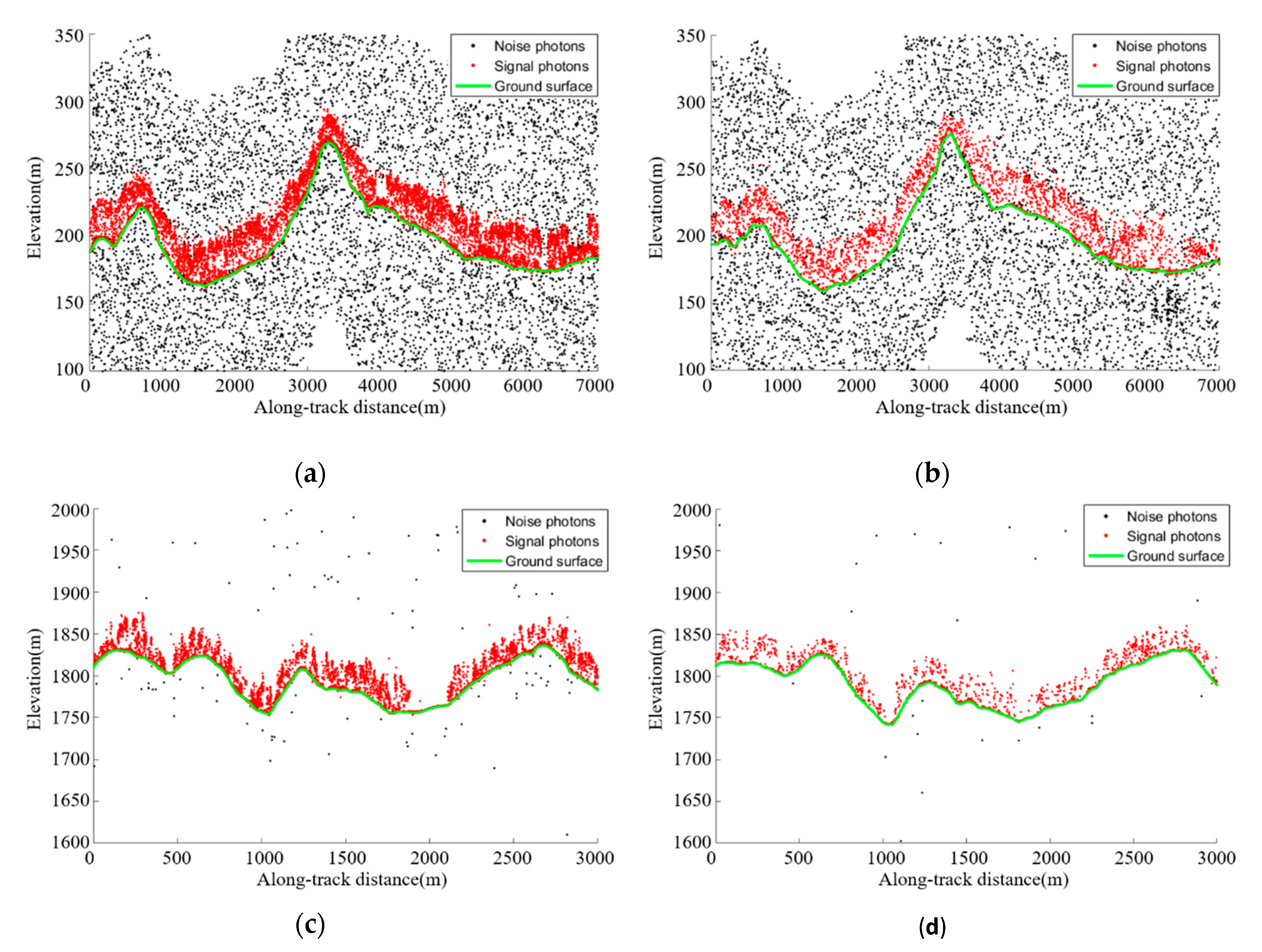
- Ground surface extraction. There are four key steps to implement ground surface retrieval according to our previous studies [37,47], including initial ground photon extraction, iterative detection of ground photons, ground photon densification, and ground surface fitting. First, a local elevation frequency histogram was built, and the photon at the lowest elevation peak with the maximum density was regarded as the initial ground photon. Second, the empirical mode decomposition (EMD) algorithm was utilized to eliminate wrong ground photons such as canopy photons and noise photons. Third, the number of accurate ground photons was increased based on progressive densification. Finally, all ground photons and corresponding ground surfaces were retrieved utilizing cubic spline interpolation. A more detailed description of the ground surface extraction algorithm can be found in Zhu et al. [47].
- (4)
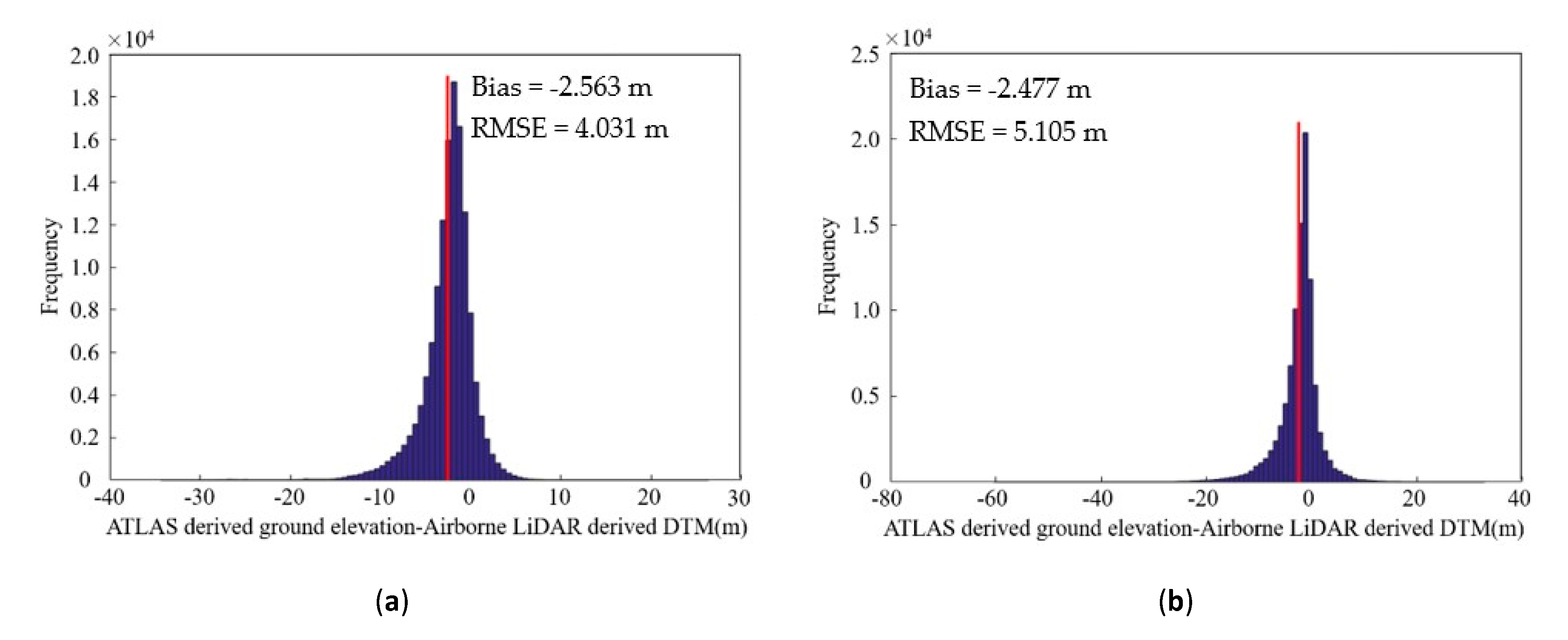
- Ground elevation validation. Once the ground surface was obtained, the airborne LiDAR-derived DTM was adopted to assess the accuracy of the ground elevation. Compared with strong beams, fewer signal photons in weak beams may reduce the accuracy of the estimated ground elevation. Additionally, photons acquired in the daytime may also introduce more solar background noises than that in the nighttime. To examine the capability of ICESat-2 data in the ground elevation estimation, the ICESat-2 data in four different scenarios were used for ground elevation estimation and validation: 1) ICESat-2 strong beams collected in the daytime, 2) ICESat-2 weak beams collected in the daytime, 3) ICESat-2 strong beams collected in the nighttime, and 4) ICESat-2 weak beams collected in the nighttime. The validation results will guide the slope estimation of ICESat-2 data.
3.2. Slope Estimation
3.2.1. Slope Estimation Method Based on Along- and Across-Track Analysis
3.2.2. Slope Estimation Method Based on Plane Fitting of Ground Track Pairs
3.3. Accuracy Validation
3.4. Error Analysis
4. Results
4.1. Validation of the Ground Elevation Accuracy
4.2. The Assessment of ICESat-2-Derived SLOPES
4.3. Error Analysis of ICESat-2 Derived Slopes
4.3.1. The Effect of Surface Topography on Terrain Slope Retrieval
4.3.2. The Effect of Ground Elevation Error on Terrain Slope Estimation
5. Discussion
5.1. Ground Surface Retrieval
5.2. The Slope Estimation from ICESat-2 Data
5.3. Error Analysis of ICESat-2 Derived Slopes
5.4. The Potential Applications of ICESat-2 Sopes
5.5. The Innovations and Limitations
6. Conclusions
Author Contributions
Funding
Conflicts of Interest
References
- Enßle, F.; Heinzel, J.; Koch, B. Accuracy of vegetation height and terrain elevation derived from ICESat/GLAS in forested areas. Int. J. Appl. Earth Obs. 2014, 31, 37–44. [Google Scholar] [CrossRef]
- González-Moradas, M.d.R.; Viveen, W. Evaluation of ASTER GDEM2, SRTMv3.0, ALOS AW3D30 and TanDEM-X DEMs for the Peruvian Andes against highly accurate GNSS ground control points and geomorphological-hydrological metrics. Remote Sens. Environ. 2020, 237, 111509. [Google Scholar]
- Wang, Z.; Li, Y.; Su, X.; Tao, S.; Feng, X.; Wang, Q.; Xu, X.; Liu, Y.; Michaletz, S.T.; Shrestha, N.; et al. Patterns and ecological determinants of woody plant height in eastern Eurasia and its relation to primary productivity. J. Plant Ecol. 2019, 12, 791–803. [Google Scholar] [CrossRef]
- Fricker, G.A.; Synes, N.W.; Serra-Diaz, J.M.; North, M.P.; Davis, F.W.; Franklin, J. More than climate? Predictors of tree canopy height vary with scale in complex terrain, Sierra Nevada, CA (USA). For. Ecol. Manag. 2019, 434, 142–153. [Google Scholar] [CrossRef]
- Liu, K.; Song, C.; Ke, L.; Jiang, L.; Pan, Y.; Ma, R. Global open-access DEM performances in Earth’s most rugged region High Mountain Asia: A multi-level assessment. Geomorphology 2019, 338, 16–26. [Google Scholar] [CrossRef]
- Muscarella, R.; Kolyaie, S.; Morton, D.C.; Zimmerman, J.K.; Uriarte, M.; Jucker, T. Effects of topography on tropical forest structure depend on climate context. J. Ecol. 2019, 108, 145–159. [Google Scholar] [CrossRef]
- Zhang, K.; Gann, D.; Ross, M.; Biswas, H.; Li, Y.; Rhome, J. Comparison of TanDEM-X DEM with LiDAR data for accuracy assessment in a coastal urban area. Remote Sens. 2019, 11, 876. [Google Scholar] [CrossRef]
- Eitel, J.U.H.; Höfle, B.; Vierling, L.A.; Abellán, A.; Asner, G.P.; Deems, J.S.; Glennie, C.L.; Joerg, P.C.; LeWinter, A.L.; Magney, T.S.; et al. Beyond 3-D: The new spectrum of lidar applications for earth and ecological sciences. Remote Sens. Environ. 2016, 186, 372–392. [Google Scholar] [CrossRef]
- Liu, X.; Hu, H.; Hu, P. Accuracy assessment of LiDAR-derived digital elevation models based on approximation theory. Remote Sens. 2015, 7, 7062–7079. [Google Scholar] [CrossRef]
- Polat, N.; Uysal, M. Investigating performance of airborne LiDAR data filtering algorithms for DTM generation. Measurement 2015, 63, 61–68. [Google Scholar] [CrossRef]
- Wessel, B.; Huber, M.; Wohlfart, C.; Marschalk, U.; Kosmann, D.; Roth, A. Accuracy assessment of the global TanDEM-X digital elevation model with GPS data. ISPRS J. Photogramm. Remote Sens. 2018, 139, 171–182. [Google Scholar] [CrossRef]
- Rizzoli, P.; Martone, M.; Gonzalez, C.; Wecklich, C.; Borla Tridon, D.; Bräutigam, B.; Bachmann, M.; Schulze, D.; Fritz, T.; Huber, M.; et al. Generation and performance assessment of the global TanDEM-X digital elevation model. ISPRS J. Photogramm. Remote Sens. 2017, 132, 119–139. [Google Scholar] [CrossRef]
- Carabajal, C.C.; Harding, D.J. ICESat validation of SRTM C-band digital elevation models. Geophys. Res. Lett. 2005, 32, L22S01. [Google Scholar] [CrossRef]
- Pham, H.T.; Marshall, L.; Johnson, F.; Sharma, A. A method for combining SRTM DEM and ASTER GDEM2 to improve topography estimation in regions without reference data. Remote Sens Environ. 2018, 210, 229–241. [Google Scholar] [CrossRef]
- Braun, A.; Fotopoulos, G. Assessment of SRTM, ICESat, and survey control monument elevations in Canada. Photogramm. Eng. Remote Sens. 2007, 73, 1333–1342. [Google Scholar] [CrossRef]
- Carabajal, C.C.; Harding, D.J. SRTM C-band and ICESat laser altimetry elevation comparisons as a function of tree cover and relief. Photogramm. Eng. Remote Sens. 2006, 72, 287–298. [Google Scholar] [CrossRef]
- Zhao, G.; Xue, H.; Ling, F. Assessment of ASTER GDEM performance by comparing with SRTM and ICESat/GLAS data in Central China. In Proceedings of the 18th International Conference on Geoinformatics, Beijing, China, 18–20 June 2010; pp. 1–5. [Google Scholar]
- Markus, T.; Neumann, T.; Martino, A.; Abdalati, W.; Brunt, K.; Csatho, B.; Farrell, S.; Fricker, H.; Gardner, A.; Harding, D.; et al. The ice, cloud, and land elevation Satellite-2 (ICESat-2): Science requirements, concept, and implementation. Remote Sens. Environ. 2017, 190, 260–273. [Google Scholar] [CrossRef]
- Wang, X.; Cheng, X.; Gong, P.; Huang, H.; Li, Z.; Li, X. Earth science applications of ICESat/GLAS: A review. Int. J. Remote Sens. 2011, 32, 8837–8864. [Google Scholar] [CrossRef]
- Nie, S.; Wang, C.; Dong, P.L.; Li, G.C.; Xi, X.H.; Wang, P.; Yang, X.B. A novel model for terrain slope estimation using ICESat/GLAS waveform data. IEEE Trans. Geosci. Remote Sens. 2017, 56, 217–227. [Google Scholar]
- Xu, L. Terrain slope estimation within footprint from ICESat/GLAS waveform: Model and method. J. Appl. Remote Sens. 2012, 6, 063534. [Google Scholar] [CrossRef]
- Mahoney, C.; Kljun, N.; Los, S.; Chasmer, L.; Hacker, J.; Hopkinson, C.; North, P.; Rosette, J.; van Gorsel, E. Slope Estimation from ICESat/GLAS. Remote Sens. 2014, 6, 10051–10069. [Google Scholar] [CrossRef]
- Li, X.; Xu, K.; Xu, L. Surface slope and roughness measurement using ICESat/GLAS elevation and laser waveform. Meas. Sci. Technol. 2016, 27, 095202. [Google Scholar] [CrossRef]
- Nie, S.; Wang, C.; Xi, X.H.; Li, G.Y.; Luo, S.Z.; Yang, X.B.; Wang, P.; Zhu, X.X. Exploring the influence of various factors on slope estimation using large-footprint LiDAR data. IEEE Trans. Geosci. Remote Sens. 2018, 56, 6611–6621. [Google Scholar] [CrossRef]
- Yi, D.; Zwally, H.J.; Sun, X. ICESat measurement of Greenland ice sheet surface slope and roughness. Ann. Glaciol. 2005, 42, 83–89. [Google Scholar] [CrossRef]
- Howat, I.M.; Smith, B.E.; Joughin, I.; Scambos, T.A. Rates of southeast Greenland ice volume loss from combined ICESat and ASTER observations. Geophys. Res. Lett. 2008, 35. [Google Scholar] [CrossRef]
- Rinne, E.; Shepherd, A.; Palmer, S.; Van Den Broeke, M.; Muir, A.; Ettema, J.; Wingham, D. On the recent elevation changes at the Flade Isblink Ice Cap, Northern Greenland. J. Geophys. Res. 2011, 116, F03024. [Google Scholar] [CrossRef]
- Li, X.; Xu, K.; Xu, L. Within-footprint roughness measurements using ICESat/GLAS waveform and LVIS elevation. Meas. Sci. Technol. 2016, 27, 125012. [Google Scholar] [CrossRef]
- Neuenschwander, A.; Pitts, K. The ATL08 land and vegetation product for the ICESat-2 Mission. Remote Sens. Environ. 2019, 221, 247–259. [Google Scholar] [CrossRef]
- Wise, B.J.A.; Thayer, J.P.; Barton-Grimley, R.A.; Gisler, A.; Anderson, C. Shallow-water bathymetry using ICESat-2 ATLAS and related LIDAR technologies. In Proceedings of the AGU Fall Meeting, San Francisco, CA, USA, 9–13 December 2019. [Google Scholar]
- Duncanson, L.; Neuenschwander, A.; Hancock, S.; Thomas, N.; Fatoyinbo, T.; Simard, M.; Silva, C.A.; Armston, J.; Luthcke, S.B.; Hofton, M. Biomass estimation from simulated GEDI, ICESat-2 and NISAR across environmental gradients in Sonoma County, California. Remote Sens. Environ. 2020, 242, 111779. [Google Scholar] [CrossRef]
- Kwok, R.; Kacimi, S.; Webster, M.; Markus, T.; Kurtz, N.T. Snow depth on Arctic sea ice from ICESat-2 and CryoSat-2. In Proceedings of the AGU Fall Meeting, San Francisco, CA, USA, 9–13 December 2019. [Google Scholar]
- Nie, S.; Wang, C.; Xi, X.H.; Luo, S.Z.; Li, G.Y.; Tian, J.Y.; Wang, H.T. Estimating the vegetation canopy height using micro-pulse photon-counting LiDAR data. Opt. Express 2018, 26, A520–A540. [Google Scholar] [CrossRef]
- Neuenschwander, A.L.; Magruder, L.A. Canopy and terrain height retrievals with ICESat-2: A first look. Remote Sens. 2019, 11, 1721. [Google Scholar] [CrossRef]
- Kwok, R.; Kacimi, S.; Markus, T.; Kurtz, N.; Studinger, M.; Sonntag, J.; Manizade, S.; Boisvert, L.; Harbeck, J. ICESat-2 surface height and sea ice freeboard assessed with ATM lidar acquisitions from Operation IceBridge. Geophys. Res. Lett. 2019, 46, 11228–11236. [Google Scholar] [CrossRef]
- Narine, L.L.; Popescu, S.C.; Malambo, L. Synergy of ICESat-2 and landsat for mapping forest aboveground biomass with deep learning. Remote Sens. 2019, 11, 1503. [Google Scholar] [CrossRef]
- Wang, C.; Zhu, X.; Nie, S.; Xi, X.; Li, D.; Zheng, W.; Chen, S. Ground elevation accuracy verification of ICESat-2 data: A case study in Alaska, USA. Opt. Express 2019, 27, 38168–38179. [Google Scholar] [CrossRef] [PubMed]
- Brunt, K.M.; Neumann, T.A.; Walsh, K.M.; Markus, T. Determination of local slope on the Greenland Ice Sheet using a multibeam photon-counting Lidar in preparation for the ICESat-2 Mission. IEEE Geosci. Remote Sens. Lett. 2013, 11, 935–939. [Google Scholar] [CrossRef]
- Neumann, T.A.; Martino, A.J.; Markus, T.; Bae, S.; Bock, M.R.; Brenner, A.C.; Brunt, K.M.; Cavanaugh, J.; Fernandes, S.T.; Hancock, D.W. The Ice, Cloud, and Land Elevation Satellite–2 mission: A global geolocated photon product derived from the advanced topographic laser altimeter system. Remote Sens. Environ. 2019, 233, 111325. [Google Scholar] [CrossRef]
- Carrasco, L.; Giam, X.; Papeş, M.; Sheldon, K. Metrics of lidar-derived 3D vegetation structure reveal contrasting effects of horizontal and vertical forest heterogeneity on bird species richness. Remote Sens. 2019, 11, 743. [Google Scholar] [CrossRef]
- Kampe, T.U.; Johnson, B.R.; Kuester, M.; Keller, M. NEON: The first continental-scale ecological observatory with airborne remote sensing of vegetation canopy biochemistry and structure. J. Appl. Remote Sens. 2010, 4, 043510. [Google Scholar] [CrossRef]
- Nie, S.; Wang, C.; Dong, P.; Xi, X.; Luo, S.; Qin, H. A revised progressive TIN densification for filtering airborne LiDAR data. Measurement 2017, 104, 70–77. [Google Scholar] [CrossRef]
- Burrough, P.A.; McDonell, R.A. Principles of Geographical Information Systems; Oxford University Press: Oxford, UK, 1998; p. 190. [Google Scholar]
- Satge, F.; Bonnet, M.P.; Timouk, F.; Calmant, S.; Pillco, R.; Molina, J.; Lavado-Casimiro, W.; Arsen, A.; Cretaux, J.F.; Garnier, J. Accuracy assessment of SRTM v4 and ASTER GDEM v2 over the Altiplano watershed using ICESat/GLAS data. Int. J. Remote Sens. 2015, 36, 465–488. [Google Scholar] [CrossRef]
- Cheung, S.; Slatton, K.C.; Cho, H.-C. Fusing landscape accuracy-dependent SRTM elevation data with NGDC and LiDAR data for the Florida coastline. Remote Sens. Lett. 2012, 3, 687–696. [Google Scholar] [CrossRef]
- Su, Y.; Guo, Q. A practical method for SRTM DEM correction over vegetated mountain areas. ISPRS J. Photogramm. Remote Sens. 2014, 87, 216–228. [Google Scholar] [CrossRef]
- Zhu, X.; Nie, S.; Wang, C.; Xi, X.; Hu, Z. A ground elevation and vegetation height retrieval algorithm using micro-pulse photon-counting lidar data. Remote Sens. 2018, 10, 1962. [Google Scholar] [CrossRef]
- Zhu, X.; Nie, S.; Wang, C.; Xi, X. The performance of ICESat-2’s strong and weak beams in estimating ground elevation and forest height. In Proceedings of the IEEE International Geoscience and Remote Sensing Symposium, IGARSS 2020, Virtual Symposium, Waikoloa, HI, USA, 26 September–2 October 2020. [Google Scholar]


| Datasets | R2 | Bias (m) | SD (m) | RMSE (m) |
|---|---|---|---|---|
| Strong beams in the daytime | 1.000 | −2.563 | 3.112 | 4.031 |
| Weak beams in the daytime | 1.000 | −2.477 | 4.464 | 5.105 |
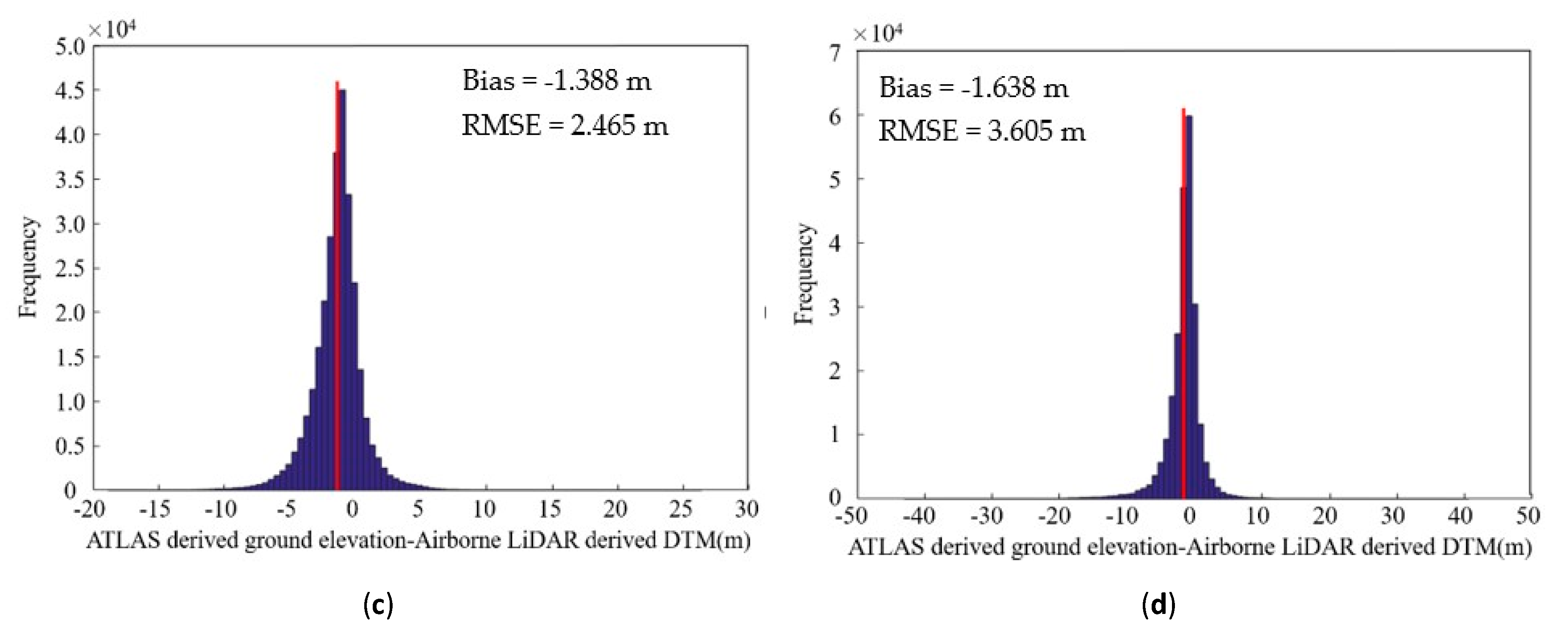
| Strong beams in the nighttime | 1.000 | −1.388 | 2.037 | 2.465 |
| Weak beams in the nighttime | 1.000 | −1.638 | 3.211 | 3.605 |
| All datasets | 1.000 | −1.816 | 3.056 | 3.555 |
| Sites | Methods | Number | Bias (°) | SD (°) | RMSE (°) |
|---|---|---|---|---|---|
| HARV | method1_All | 391 | 0.891 | 2.174 | 2.347 |
| method1_Strong | 201 | 0.630 | 2.123 | 2.210 | |
| method1_Weak | 190 | 1.168 | 2.199 | 2.485 | |
| method 2 | 201 | 0.805 | 1.332 | 1.553 | |
| SCBI | method1_All | 1204 | −0.086 | 2.870 | 2.870 |
| method1_Strong | 602 | −0.116 | 2.879 | 2.879 | |
| method1_Weak | 602 | −0.056 | 2.863 | 2.862 | |
| method 2 | 602 | −0.270 | 2.108 | 2.124 | |
| SJER | method1_All | 1752 | −0.399 | 3.304 | 3.327 |
| method1_Strong | 876 | −0.558 | 3.146 | 3.193 | |
| method1_Weak | 876 | −0.240 | 3.450 | 3.456 | |
| method 2 | 876 | −0.780 | 2.128 | 2.265 | |
| SOAP | method1_All | 1564 | −0.773 | 4.327 | 4.394 |
| method1_Strong | 782 | −0.617 | 4.201 | 4.243 | |
| method1_Weak | 782 | −0.929 | 4.446 | 4.539 | |
| method 2 | 782 | −0.769 | 2.828 | 2.929 | |
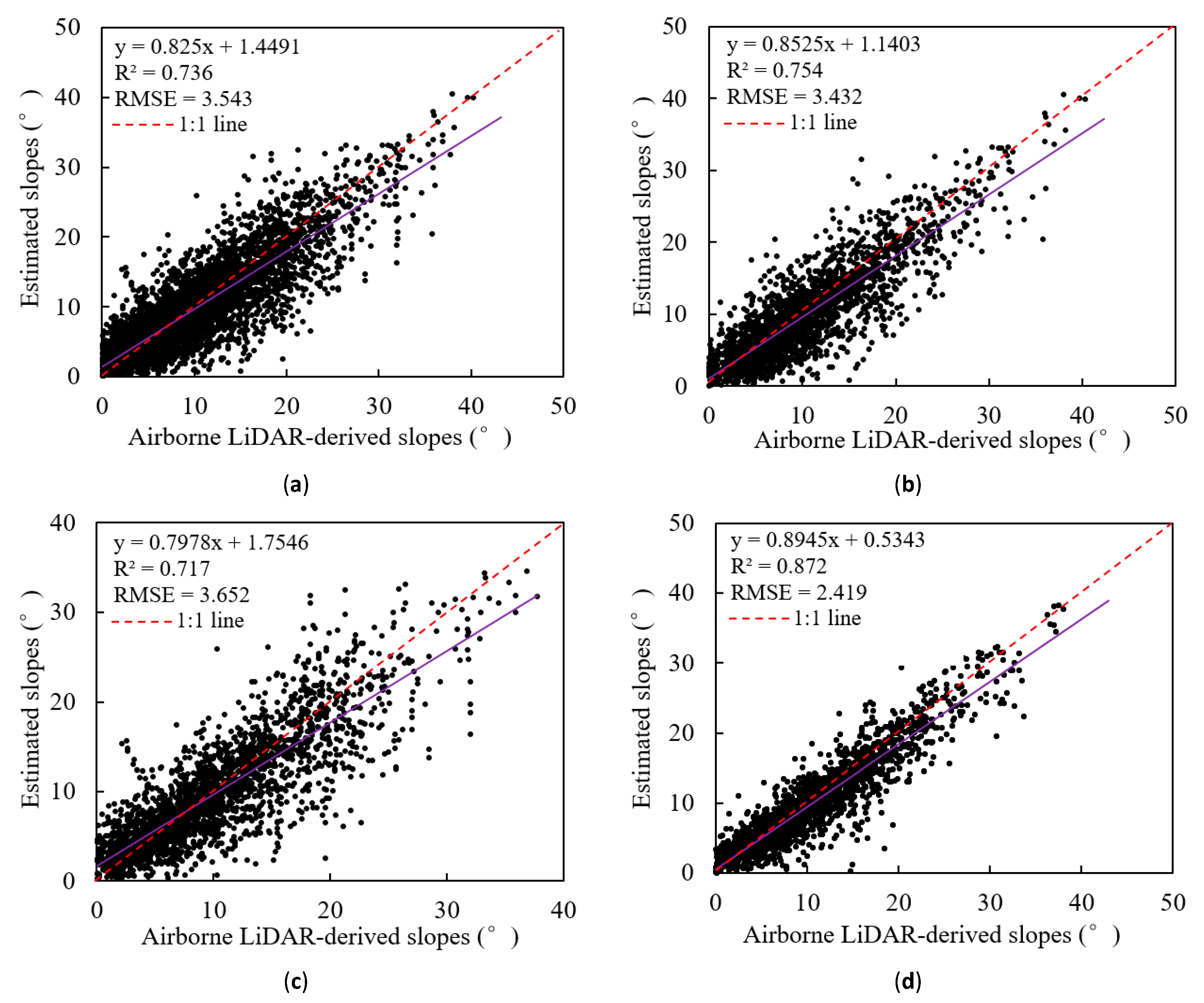
| All | method1_All | 4911 | −0.339 | 3.528 | 3.543 |
| method1_Strong | 2461 | −0.371 | 3.412 | 3.432 | |
| method1_Weak | 2450 | −0.306 | 3.640 | 3.652 | |
| method 2 | 2461 | −0.522 | 2.363 | 2.419 |
| Data Time | Methods | Number | Bias (°) | SD (°) | RMSE (°) |
|---|---|---|---|---|---|
| Daytime | method1_All | 1462 | −0.752 | 4.311 | 4.374 |
| method1_Strong | 731 | −0.582 | 4.198 | 4.236 | |
| method1_Weak | 731 | −0.922 | 4.417 | 4.509 | |
| method 2 | 731 | −0.769 | 2.831 | 2.932 | |
| Nighttime | method1_All | 3449 | −0.163 | 3.121 | 3.125 |
| method1_Strong | 1730 | −0.282 | 3.016 | 3.028 | |
| method1_Weak | 1719 | −0.043 | 3.220 | 3.220 | |
| method 2 | 1730 | −0.418 | 2.126 | 2.166 |
| Methods | Slope Errors | ICESat-2 Slopes | SRTM-Derived Slopes | GDEM-Derived Slopes |
|---|---|---|---|---|
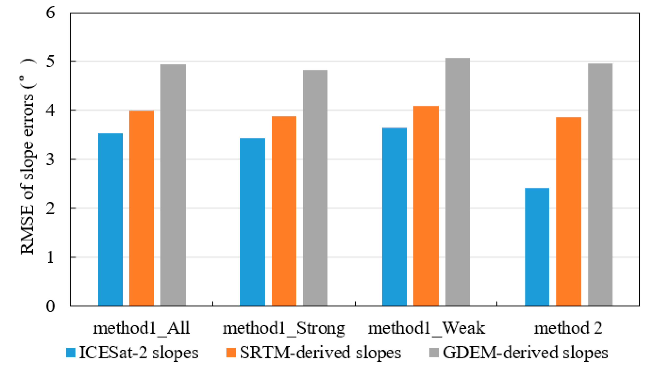
| method1_All | R2 | 0.736 | 0.676 | 0.592 |
| Bias | −0.339 | −0.928 | 1.125 | |
| SD | 3.528 | 3.883 | 4.822 | |
| RMSE | 3.543 | 3.992 | 4.951 | |
| method1_Strong | R2 | 0.754 | 0.692 | 0.607 |
| Bias | −0.371 | −0.935 | 1.062 | |
| SD | 3.412 | 3.770 | 4.705 | |
| RMSE | 3.432 | 3.884 | 4.822 | |
| method1_Weak | R2 | 0.717 | 0.660 | 0.577 |
| Bias | −0.306 | −0.92 | 1.194 | |
| SD | 3.640 | 3.994 | 4.942 | |
| RMSE | 3.652 | 4.097 | 5.083 | |
| method 2 | R2 | 0.872 | 0.681 | 0.573 |
| Bias | −0.522 | −0.868 | 1.064 | |
| SD | 2.363 | 3.766 | 4.837 | |
| RMSE | 2.419 | 3.864 | 4.952 |
| Methods | Slope Errors (°) | Slope (°) | |||
|---|---|---|---|---|---|
| 0–5 | 5–10 | 10–15 | >15 | ||
| method1_All | Number | 1217 | 1533 | 1097 | 1064 |
| Bias | 1.208 | −0.076 | −0.768 | −2.043 | |
| SD | 2.340 | 2.842 | 3.451 | 4.621 | |
| RMSE | 2.633 | 2.842 | 3.534 | 5.051 | |
| method1_Strong | Number | 573 | 817 | 553 | 518 |
| Bias | 1.002 | −0.172 | −0.672 | −1.885 | |
| SD | 2.330 | 2.957 | 3.436 | 4.294 | |
| RMSE | 2.535 | 2.960 | 3.498 | 4.685 | |
| method1_Weak | Number | 644 | 716 | 544 | 546 |
| Bias | 1.392 | 0.033 | −0.866 | −2.194 | |
| SD | 2.335 | 2.702 | 3.467 | 4.911 | |
| RMSE | 2.717 | 2.700 | 3.570 | 5.374 | |
| method 2 | Number | 617 | 782 | 559 | 503 |
| Bias | 0.465 | −0.405 | −0.884 | −1.513 | |
| SD | 1.462 | 1.937 | 2.417 | 3.171 | |
| RMSE | 1.533 | 1.977 | 2.572 | 3.511 | |
| Methods | Slope Errors (°) | RMSE of Ground Elevation Errors (m) | |||
|---|---|---|---|---|---|
| 0–1 | 1–2 | 2–3 | >3 | ||
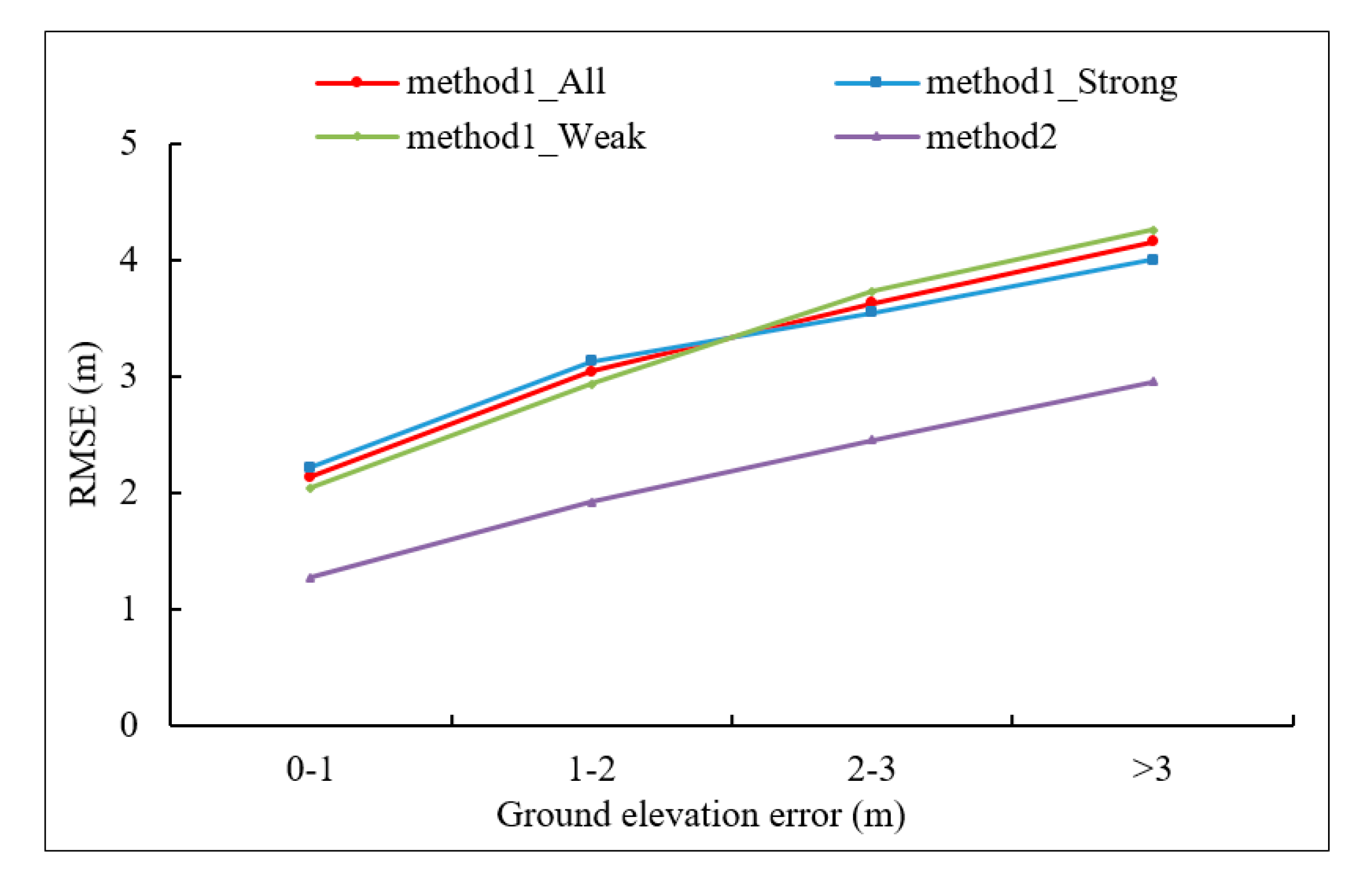
| method1_All | Number | 490 | 1556 | 1133 | 1732 |
| Bias | 0.313 | −0.320 | −0.543 | −0.406 | |
| SD | 2.120 | 3.032 | 3.597 | 4.141 | |
| RMSE | 2.141 | 3.048 | 3.637 | 4.160 | |
| method1_Strong | Number | 260 | 877 | 628 | 696 |
| Bias | 0.010 | −0.366 | −0.383 | −0.511 | |
| SD | 2.225 | 3.114 | 3.536 | 3.974 | |
| RMSE | 2.220 | 3.133 | 3.554 | 4.004 | |
| method1_Weak | Number | 230 | 679 | 505 | 1036 |
| Bias | 0.656 | −0.261 | −0.743 | −0.335 | |
| SD | 1.943 | 2.925 | 3.665 | 4.251 | |
| RMSE | 2.047 | 2.935 | 3.736 | 4.262 | |
| method 2 | Number | 286 | 664 | 462 | 801 |
| Bias | −0.096 | −0.392 | −0.663 | −0.614 | |
| SD | 1.276 | 1.885 | 2.370 | 2.899 | |
| RMSE | 1.278 | 1.924 | 2.459 | 2.962 | |
© 2020 by the authors. Licensee MDPI, Basel, Switzerland. This article is an open access article distributed under the terms and conditions of the Creative Commons Attribution (CC BY) license (http://creativecommons.org/licenses/by/4.0/).
Share and Cite
Zhu, X.; Nie, S.; Wang, C.; Xi, X.; Li, D.; Li, G.; Wang, P.; Cao, D.; Yang, X. Estimating Terrain Slope from ICESat-2 Data in Forest Environments. Remote Sens. 2020, 12, 3300. https://doi.org/10.3390/rs12203300
Zhu X, Nie S, Wang C, Xi X, Li D, Li G, Wang P, Cao D, Yang X. Estimating Terrain Slope from ICESat-2 Data in Forest Environments. Remote Sensing. 2020; 12(20):3300. https://doi.org/10.3390/rs12203300
Chicago/Turabian StyleZhu, Xiaoxiao, Sheng Nie, Cheng Wang, Xiaohuan Xi, Dong Li, Guoyuan Li, Pu Wang, Di Cao, and Xuebo Yang. 2020. "Estimating Terrain Slope from ICESat-2 Data in Forest Environments" Remote Sensing 12, no. 20: 3300. https://doi.org/10.3390/rs12203300
APA StyleZhu, X., Nie, S., Wang, C., Xi, X., Li, D., Li, G., Wang, P., Cao, D., & Yang, X. (2020). Estimating Terrain Slope from ICESat-2 Data in Forest Environments. Remote Sensing, 12(20), 3300. https://doi.org/10.3390/rs12203300


