Abstract
This paper presents an ice classification algorithm based on combined active and passive microwave radiometer data in Lützow-Holm Bay (LHB), East Antarctica. The ice classification algorithm is developed based on the threshold values of an advanced scatterometer (ASCAT) and advanced microwave scanning radiometer 2 (here, AMSR2). These values are calculated via the features of various ice types, including open ice, first-year (FY) ice, multi-year (MY) ice, MY ice including icebergs (MY IB), ice shelves, coastal ice sheets, and inland ice sheets. To verify the validity of the ice classification algorithm, the algorithm results are compared with visual observation data and satellite imagery. Except for the flaw polynya and area with surface melting, the FY ice, MY ice, and the ice shelf areas estimated here using the proposed ice classification algorithm match those discernible from the verification data. Inter-annual changes in the areal extents of FY ice, MY ice, and the ice shelves are investigated here using the proposed ice classification algorithm. Investigation of MY ice and ice shelf areas revealed that the breakup of MY ice induced a breakup of an ice shelf. A comparison of the FY ice and MY ice areas showed the replacement of these ice types. The proposed ice classification algorithm can detect ice breakup events as quantitative changes in the distribution and ice type. In future work, we plan to classify sea ice in other sea ice areas, applying the proposed algorithm throughout the Antarctic region.
1. Introduction
Sea ice plays an important role in both surface atmosphere heat exchange and oceanic thermohaline circulation. Since 1979, the spatial extent of Antarctic sea ice has been observed by satellite-based passive microwave remote sensing with the maximum sea ice extent recorded during 2012–2014 [1]. Importantly, the minimum sea ice extent was recorded in 2016 [2]. In contrast to the areal extent, the spatial and temporal distributions of sea ice thickness in the Antarctic remain largely unknown [3]. The quantification of sea ice thickness is of crucial importance, as when combined with data on the areal extent, this information enables the computation of sea ice volume. Knowledge about sea ice volume can provide insight into both the heat budget of the Antarctic sea ice system and the quantification of fresh water and saltwater fluxes into the Southern Ocean.
Satellite-based remote sensing techniques, such as satellite altimeters, have been developed in recent years to collect long-term extensive datasets of distributions of sea ice thickness. Altimetric observation of sea ice thickness is based on freeboard measurements, that is, the height of an ice floe above the sea surface, which can be used to calculate ice thickness values [4]. Data about the sea ice, snow, and sea water density are required for sea ice thickness estimation by satellite altimeter measurements. A current satellite altimeter, Cryosat-2 (CS-2), was launched in April 2010 by the European Space Agency (ESA), and CS-2 data of the freeboard and sea ice thickness in the Arctic region have been made available to the public by the Alfred Wegener Institute. Additionally, the verification of freeboard estimation is being carried out in the Southern Ocean [5]. However, estimation methods of sea ice thickness have not yet been established. This is because, as mentioned above, information about sea ice density is essential for altimetric sea ice thickness estimation. Sea ice density changes between first-year (FY) ice and multi-year (MY) ice, as the volume of brine contained in sea ice changes over time. Therefore, it is necessary to establish a sea ice classification method for ice thickness estimation using an altimeter.
The Antarctic sea ice zone is composed of a complex mixture of ice of different types with variable thickness, the surface of which is generally covered by snow with variable thickness. Each austral autumn, drift ice covers the Southern Ocean’s seasonal ice zone away from the coastal regions, while fast ice forms around much of the Antarctic continent. At a maximum, fast ice can account for as much as 14% (by area) of East Antarctic sea ice [6]. As fast ice is typically fixed along the continent, this makes it an ideal target for studies of ocean ice atmosphere interaction with a focus on thermodynamic processes [7]. Moreover, the presence of drift ice and fast ice in coastal areas is also important for understanding the causes of ice shelf collapse, with the aim of improving models of the Antarctic ice sheet and predicting the future behaviors of these ice sheets and their related contributions to sea level rise [8].
Various studies have been conducted to classify ice types using satellite remote sensing. For example, Tamura et al. [9] developed an algorithm to classify drift ice, fast ice (including glacier tongues, grounded icebergs, and ice shelves), and continental ice using a satellite passive microwave radiometer, namely the Special Sensor Microwave Imager (SSM/I). Aulicino et al. [10] developed an algorithm for the classification of sea ice types using satellite passive microwave radiometer data (collecting using the Advanced Microwave Scanning Radiometer for the Earth Observing System (AMSR-E) instrument) collected during the winter season. A method for classifying ice types in the Antarctic Ocean in winter was developed using the backscattering coefficient measured by the satellite-based scatterometer on European Remote Sensing Satellite 1 (ERS-1) [11]. Satellite scatterometers are primarily designed to provide a global ocean wind vector data. The characteristics and melting processes of the Antarctic sea ice surface of MY ice have been investigated using satellite scatterometer data obtained by ERS-1/-2 [12]. A sea ice detection algorithm was developed using an advanced scatterometer (ASCAT) with Bayesian estimation [13]. Additionally, a method using the backscattering coefficient measured by ASCAT and a passive microwave radiometer (Special Sensor Microwave Imager Sounder (SSMIS)) has also been developed and published as a product for use in the Arctic [14]. Although methods for classifying ice around the continent have been developed, no algorithms have yet been developed for both the Arctic and Antarctic that can accurately distinguish between FY ice, MY ice, ice shelves, and ice sheets at the same time.
Figure 1a shows a map of eastern Antarctica, and the area marked in a grid pattern corresponds to the area in Figure 1b. In the current study, an ice classification algorithm was constructed for use with data from Lützow-Holm Bay (LHB), located at approximately 69° S, 38° E, located near the eastern of Queen Maud Land (Figure 1b). The Japanese icebreaker Shirase, with the Japanese Antarctic Research Expedition (JARE), sets out for the Syowa Station at approximately the same time every year. Visual observation and sea ice observation using a measuring instrument is carried out along the track of the ship [15]. The compositions of ice around LHB are described below. Most of the area is covered with fast ice, and drift ice is located north of 68.5° S. A flaw polynya called “Otone-Suiro” frequently appears at the boundary between the drift ice and the fast ice. Here, a flaw polynya refers to the narrow separation zone between drift ice and fast ice that forms when drift ice shears under the effects of a strong wind or current along the fast ice boundary [16]. The ice composition includes an ice shelf, the Shirase Glacier (SG), and ice sheets bordering the coastline. Usually, the fast ice tends to form along the edge of the continental ice shelf. However, the passage of atmospheric low-pressure systems can trigger the breakup of fast ice [17]. Moreover, Aoki [18] investigated the relationship between ice breakup latitude and various variables, revealing that the breakup latitude in April had a persistently high correlation with the sea surface temperature (SST) in the tropical Pacific Ocean. In the current study, we focused on the large-scale breakups of ice in LHB, attempting to clarify the underlying mechanisms, as described above. Fast ice breakups may replace MY ice with FY ice. In the current study, we compared these two types of ice before and after breakup.
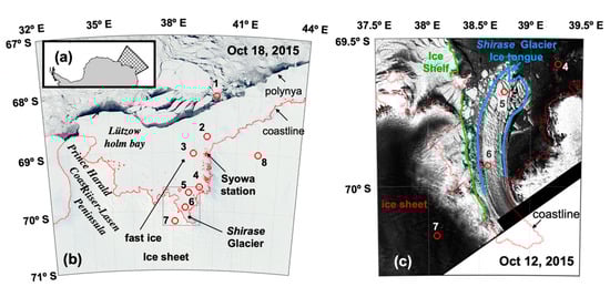
Figure 1.
Ice conditions in Lüzow-Holm Bay, East Antarctica, and surrounding areas: (a) Map of eastern Antarctica and (b) an overall view of Lützow-Holm Bay from an Aqua Moderate Resolution Imaging Spectroradiometer (MODIS) image acquired on 18 October 2015. (c) An enlarged view around the Shirase glacier tongue provided by a Sentinel-1 C-band synesthetic aperture radar (C-SAR) image acquired on 12 October 2015. The reference points intended to represent the five types of ice identified in the MODIS images, which include the following: (1) Drift ice, (2) multi-year fast ice including grounded icebergs, (3) first year fast ice, (4) multi-year fast ice, (5) tip of the Shirase Glacier tongue, (6) main part of the Shirase Glacier tongue, (7) a coastal ice sheet, and (8) an inland ice sheet.
This paper presents an ice classification algorithm based on combined microwave radiometer and scatterometer data from LHB, as well as the results of verification tests of this algorithm. Briefly, the algorithm considers the annual variation of the normalized radar cross section (σ0) of each ice type in LHB measured by ASCAT with threshold values for the ice classification scheme identified on the basis of simple supervised clustering analysis [11]. To verify the validity of the classification, the results are compared with ship-based visual observations and satellite images. The remainder of the paper is structured as follows. Section 2 describes the data and data sources used in this study. Section 3 describes the annual tendency of satellite data and the classification workflow. Section 4 presents the results of the ice classification and discusses the reliability of the proposed algorithm. Section 5 discusses changes in the considered ice areas before and after a large-scale breakup based on the results of the algorithm. Section 6 presents our conclusions and possibilities for future research.
2. Materials and Methods
A summary of the data types and sources used in this study is presented in Table 1. In the current study, ice types were classified based on several satellite datasets, and these datasets are described below.

Table 1.
Summary of the satellite data products. ASCAT: Advanced scatteromter; SIR: Scatterometer image reconstruction; MODIS: Moderate Resolution Imaging Spectroradiometer.
The following data sources were used to develop the algorithm. Normalized radar cross section (σ0) data were derived from the ASCAT instrument. The sea ice concentration (SIC) and brightness temperature (TB) products derived from AMSR2 were used to detect the presence of sea ice and surface melting, respectively. Sentinel-1 grayscale intensity imagery and Moderate Resolution Imaging Spectroradiometer (MODIS) visible imagery were used to verify the validity of the proposed algorithm. In the following subsections, each dataset is described in more detail.
2.1. Advanced Scatterometer (ASCAT)
ASCAT was primarily designed to provide global ocean wind vectors operationally. ASCAT is an active microwave advanced scatterometer mounted onboard the polar-orbiting satellites MetOp-A and MetOp-B, which are operated by the European Organization for the Exploitation of Meteorological Satellites, and these satellites were launched in 2006 and 2012, respectively. The ASCAT instrument can transmit pulses with vertical co-polarization (VV) operating in the C-band at 5.255 GHz. The ASCAT instrument has two sets of three fan-beam antennae that measure the returned backscatter signal at incident angles of 25–65°. The antennae extend to either side of the instrument, resulting in a double swath of observations, each 550 km wide, separated by a gap of approximately 360 km [19]. The microwave pulses can penetrate clouds and are not dependent on solar illumination, meaning that ASCAT can provide daily “all-condition” surface measurements and imaging covering approximately 80% of the globe [20]. ASCAT’s standard backscatter product has a nominal spatial resolution of 25 or 50 km with very high temporal resolution (i.e., multiple passes per day). However, to investigate the small-scale ice area considered in this study, we used a scatterometer image reconstruction (SIR) algorithm, specifically a 4.45-km resolution all-passes product that is a composite of several passes over the pole during a day [21]. This enhanced resolution product was provided by the Brigham Young University Microwave Earth Remote Sensing Laboratory [22]. All backscattering data were processed using the SIR algorithm [23], which uses multiple days of scatterometer data to create a grid-like resolution enhancement product. This algorithm assumes a linear model that relates the normalized radar cross section (σ0) to the signal incident angle (θ):
σ0 = A + B (θ − 40).
The model normalizes the incident angle to 40°. This will create two images, referred to as image A (including normalized backscattering values, in dB) and image B (representing the incident angle dependence of backscattering, in dB/°). In this study, image A of the v-polarization evening pass was utilized.
2.2. Advanced Microwave Scanning Radiometer 2 (AMSR2)
AMSR2 is the passive microwave radiometer instrument mounted onboard the Global Change Observation Mission Water (GCOM-W) satellite, which was launched in May of 2012. The AMSR2 instrument is a conical scanning passive microwave radiometer system that measures in seven frequency bands (in the range of 6.925–89.0 GHz) in both horizontal and vertical polarizations. The antenna’s different feedhorns scan at an incidence angle of 55° and provide a 1450 km swath of coverage at the Earth’s surface. Here, we used descending passes to find TB values for each frequency and polarization. Additionally, SIC values are provided as 10-km gridded data on a polar stereographic projection from the Japan Aerospace Exploration Agency (JAXA) as the AMSR2 Level 3 (L3) products.
As the value of σ0 is sensitive to melting of the snow or ice surface [20], melting represents a source of error. In the current study, surface melting was detected using the following procedure. Combining TB values at different frequencies and polarizations enables different stages of melting progression to be distinguished [24]. The combination of the horizontally polarized TB at 19 GHz (TB 19H) and the vertically polarized TB at 37 GHz (TB 37V) is the most sensitive index for detecting surface and subsurface melting. As snowmelt water drains from the upper snow cover to deeper layers, the emissivity of TB 19H increases and can even exceed the emissivity of TB 37V.
Therefore, the cross-polarization ratio (XPR) can be used as an index to determine whether melting has occurred in the surface or in the subsurface layer. Arndt et al. [25] represented these combinations of TB 19H and TB 37V derived from the passive microwave radiometers SSM/I and SSMIS mounted onboard the Defense Meteorological Satellite Program (DMSP) satellites via the XPR, which is expressed using the following equation:
XPR = TB 19H • TB 37V−1.
As the brightness temperature frequencies measured by the AMSR2 sensor were 18 and 36 GHz, the XPR was calculated in this study by replacing TB 19H with TB 18H and TB 37V with TB36V.
Markus and Burns [26] developed a polynya estimation model using the polarization ratio (PR) between 37 and 85 GHz, sensed by SSM/I. Moreover, the frequency of 36 GHz is affected by the open water fraction [27]. In this study, PR36, calculated using the following equation was used for identifying drift ice of different concentrations.
PR36 = (TB 36V − TB 36H) • (TB 36V + TB 36H))−1
In this study, the PR36 and XPR values were calculated using TB 18H, TB 36V, and TB 36H of the AMSR2 L3 product.
2.3. MODIS Imagery
The MODIS instruments onboard the Terra and Aqua spacecraft provide a wealth of spectral and spatial information about the Earth. One of the most aesthetically pleasing MODIS products is the true color images (also known as natural color images) of the Earth at a 250-m spatial resolution. MODIS is the first orbiting imaging sensor to provide such images at a reasonably high spatial resolution over a wide swathe. In the current study, we used MODIS-corrected reflectance true color GeoTIFF imagery to validate the classification results. The MODIS Imagery products were obtained from the NASA’s Earth Observing System Data and Information System (EOSDIS). Additionally, EODIS publishes coastline data via OpenStreetMap. In the current study, coastline data were used to classify areas of land and sea.
2.4. Sentinel-1 Level 1 Product
Sentinel-1 was launched on the 3rd of April 2014, from Kourou Spaceport in French Guiana. Data became operationally available around October of 2014, following a commissioning phase. The main instrument of Sentinel-1 is a C-band synesthetic aperture radar (C-SAR) instrument, which provides data in the form of SAR images with various modes and resolutions. Hereafter, C-band SAR images are referred to as C-SAR images for simplicity. For operational large-scale ice areas, we used the ground range detected extended wide swath mode at a medium resolution (93 × 87 m) corresponding to an equivalent number of looks of 12.7. Data were provided with 40 × 40 m pixel spacing. Sentinel-1 level 1 products were provided by the ESA’s Copernicus Open Access Hub.
3. Annual Trends in Normalized Radar Cross Section (σ0)
3.1. Definition of Ice Type
In this section, to develop the ice classification algorithm using data from ASCAT and AMSR2, the annual variation of σ0, XPR, and SIC at the eight points (shown in Figure 1b) was investigated. It should be noted that the images show ice conditions as of October of 2015. As will be described later, ice distributions may be substantially altered through sea ice breakup. Hereafter, each point in Figure 1b is referred to by its location number. In the current study, seven ice types (drift ice, first-year (FY) fast ice, second year (SY) fast ice, multi-year (MY) fast ice, ice shelves, coastal ice sheets, and inland ice sheets) were defined using classification from MODIS visible true color imagery and Sentinel-1 C-SAR grayscale reflectance intensity images between October of 2012 and December of 2018.
Ice that had drifted without sticking to the coast was defined as drift ice. Drift ice is represented by location 1 in Figure 1b, which is covered by various types of ice floes in austral winter and open water in austral summer. In this study, the drift ice area was defined in the following two sea ice types using the sea ice concentration. Areas where SIC was 15% or more and less than 70% were defined as open ice, and an area with value of 70% or more was defined as pack ice. Here, these ice types refer to the WMO’s sea ice nomenclature [16]. From the MODIS images for multiple years, ice attached to the coastline was defined as fast ice. Fast ice was further categorized as FY fast ice, i.e., ice which has not survived the summer melting season, and MY fast ice, which remains for multiple years. Location 3 in Figure 1b is the representative point of FY fast ice, where breakup and recovery were constantly repeated every year, except 2014. Locations 2 and 4 in Figure 1b are the representative points of MY fast ice before large-scale breakup in 2016. The details of this large-scale breakup will be explained in the next subsection. Location 2 is the point at which the grounded icebergs are embedded in the fast ice, and this was confirmed from the MODIS and C-SAR images. Location 5 indicates the tip of the ice tongue of the SG. The SAR image shown in Figure 1c indicates that the tip of the ice tongue is comprised of multiple icebergs. Location 6 indicates the main part of ice tongue of the SG. The backscatter intensity of the SG was higher than that of location 4. Additionally, the image shows the ice shelf area on the western side of the SG. The area on the continent side of the coastline of the MODIS image was defined as the ice sheet. This coastline was also used to distinguish the ice sheets from the ice shelves and sea ice. Locations 7 and 8 represent coastal and inland ice sheets, respectively.
3.2. Temporal Variations of Backscatter Coefficient (σ0)
This section describes the temporal variation of σ0, derived from the ASCAT, SIC, and surface melting derived from AMSR2 at the points shown in Figure 1b,c. First, the large-scale breakup in 2016 is explained by the MODIS images. Figure 2 shows the breakup process of the fast ice in the LHB in 2016. Figure 2a,b shows the ice before and after the breakup in the LHB, respectively. Before the breakup, the entire LHB area was covered with fast ice. The MY fast ice expanded in the area, ranging from location 3 to location 4 and 5. However, it can be confirmed from Figure 2b that gray-white ice formed in LHB. However, near location 2, the whole fast ice did not flow out and remained after breakup, as shown in Figure 2b. In just 2 months from February of 2016, most of the fast ice broke up to the north of locations 4 and 5, and most of the MY fast ice flowed out from LHB. After the passing of MY fast ice, FY ice grew in this region. In other words, the type of ice changed after the breakup. Additionally, sea ice breakup occurred in years other than 2016. The southern limit edge of breakups in 2012, 2013, and 2015 was to the south of location 3. After these breakups, the ice in location 3 was confirmed to be FY fast ice by MODIS images. In 2017, the ice to the south of locations 4 and 5 flowed outwards. In 2018, FY fast ice flowed outwards to the north of both points.
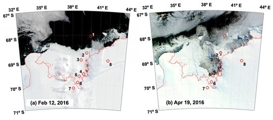
Figure 2.
Time series of the spatial distribution of sea ice based on MODIS imagery for (a) February 12, and (b) April 21 in 2016.
Figure 3 shows the time series of σ0 at eight locations, as shown in Figure 1, indicated by a solid line, and the surface melting determined from the XPR is indicated by a gray shading. The dashed line in Figure 3a shows the SIC. It should be noted that the time series data are not values averaged over the circles, but those from a satellite image pixel at their center, as shown in Figure 1. Analyzing the MODIS imagery and the Sentinel imagery across multiple years, the ice conditions were investigated at each location. The resulting ice types are indicated here by horizontal bars over the period of their existence. These bars also show the time periods extracted to calculate the thresholds for classifying each ice type. The types of ice are shown in the lower legend of Figure 3. The behavior of σ0 during melting is explained in the next subsection.
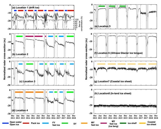
Figure 3.
Time series of ASCAT σ0 and sea ice concentration (SIC) from October 2012 to September 2018 for the eight locations in the Antarctic coastal area shown in Figure 1. The black bold lines donate the σ0 value for each ice area. The black dashed line, which is only shown in (a), is the SIC, and the gray shading indicates time periods of continuous snow melting on the sea ice. The broken vertical line indicates a major period of breakup in Lützow-Holm bay. The colored horizontal bar indicates the type of ice and over the period of their existence, as well as the time periods extracted to calculate the threshold for classifying each type of ice.
In location 1, which represents drift ice, the variation of σ0 was larger than that in other ice areas, particularly in the summer season. Conversely, the value of σ0 in other seasons was relatively stable. The standard deviation of σ0 at location 1 was 3.2 dB in summer and 1.1 dB in winter. The SIC is close to zero during the period when the variation of σ0 is large. We consider that large variations may be attributed to waves due to the absence of sea ice. Conversely, σ0 is considered to be relatively stable in winter because of the presence of sea ice.
The broken vertical lines represent the times at which a large ice breakup occurred over several years at locations 2, 3, and 4. After sea ice breakup, σ0 tends to decrease sharply. As mentioned above, MY or SY fast ice is replaced by FY fast ice when breakups occur. In other words, σ0, both before and after a breakup, may be associated with those ice types.
At location 2, the value of σ0 increased during 2012–2014, except during the melting season. The average value of σ0 in 2014 and 2015 was −8 dB, which is stable. Additionally, as shown in Figure 3d, the average value of σ0 was −10 dB from 2013 to 2015, which is also stable. Even with the same MY fast ice, the value of σ0 was higher in location 2, which includes grounded icebergs.
The value of σ0 was highest in the area covered by the SG ice tongue at the locations 5 and 6, particularly at location 5, which is located at the tip of the SG’s ice tongue. In the first year after the large-scale break up event, σ0 decreased to the same level as the MY fast ice in 2017. The broken line in Figure 3e shows the time at which the tip of the ice tongue broke up. This breakup was confirmed from the C-SAR images in 2017. The decrease in the value of σ0 after the ice tongue breakup will be discussed later. Location 7 is a coastal ice sheet, and σ0 was stable at −11 dB there, except in summer, as shown in Figure 3g. Additionally, σ0 was lower than the coastal ice sheet at location 8, as shown in Figure 3h. This may be due to the outflow velocity difference between the coastal ice sheet and the inland ice sheet.
3.3. Changes in σ0 Caused by Surface Melting
The onset of surface melting coincided with a rapid decrease of σ0 in MY fast ice and a rapid increase in FY fast ice. Moreover, the behavior of σ0 during melting seasons tended to differ between FY fast ice and MY fast ice. The difference in the behavior of σ0, depending on the age of the ice in the melting season, can be explained as follows. In MY fast ice, the onset of melting is indicated by a sharp decrease in σ0. The causative mechanism is the absorption of microwave energy by liquid water within the snow cover [28]. Increasing the dielectric constant, particularly dielectric loss, effectively masks the volume scattering of hummock ice, thereby reducing σ0. In other words, the reduction of σ0 progresses with both the pendular and funicular regimes of snow ablation [11]. Furthermore, according to Kawamura et al. [29], a sharp increase in the backscattering coefficient may be caused by superimposed ice formed by the freezing of water in the snow during the refreezing process. The gradual decline during winter may be related to the flooding and refreezing of the surface layer, reducing the surface roughness of the snow–ice interface. Conversely, in FY fast ice, melt onset is indicated by a sharp increase in σ0. Generally, FY fast ice has thinner snow cover than MY fast ice. A likely cause for this observation is the presence of particles of wet snow in the basal layer with relatively low water volumes (1–3%). These particles are large and thereby may significantly contribute to raising the value of σ0.
3.4. Developing Ice Type Classification Algorithm
Figure 4a shows the ice classification flow developed from the characteristics of σ0, derived from the ASCAT, SIC, XPR, and PR36 calculated from AMSR2, and the coastal line from the MODIS imagery, described in the previous sections. Figure 4b presents a table summarizing the ice types that were classified in this study and the WMO’s additional types of sea ice included in the aforementioned ice types. An early attempt at one-dimensional classification for Antarctic ice was based on simple supervised clustering analysis using EScat backscatter statistics [11]. In the current study, the validity of the sea ice threshold values was compared with the results of a previous study by Drinkwater [11].
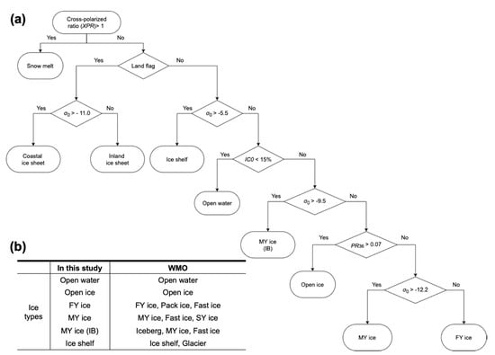
Figure 4.
(a) Workflow for the ice classification algorithm based on the σ0 values, brightness temperature (TB), and sea ice concentration (SIC) data. (b) Table summarizing the different ice types defined in this study and the WMO’s defined ice types. FY: First-year; MY: Multi-year; IB: Iceberg; SY: Second-year. XPR: Cross-polarization ratio.
3.4.1. Surface Melting
First, surface melting was determined using the index defined by the XPR > 1 [25]. As mentioned in Section 3.4, the behavior of σ0 during the melting period is complex and has temporal dependency. Moreover, it differs between ice types. Thus, unfortunately, ice classification cannot be performed during the melting period.
3.4.2. Ice of Land Origin
Next, ice of land origin and sea ice areas were classified using the coastal line derived from the MODIS images. Regions in which the value of σ0 was greater than −11.0 dB were defined as coastal ice sheets, as shown in Figure 3g; otherwise, the given region was defined as an inland ice sheet. The threshold values were determined based on the average values of the coastal ice sheets and inland ice sheets, excluding the melting season. Ice regions at sea where σ0 exceeded −5.5 dB were defined as an ice shelf. This includes SG ice tongue. This threshold value was determined based on the average values of location 5, as shown in Figure 3e. This threshold value was also used for classifying icebergs in the study by Drinkwater [11]. This threshold value is appropriate because icebergs are composed of ice originating from an ice shelf.
3.4.3. Sea Ice
Next, the classification of sea ice is described. Figure 5 shows a scatter plot with histograms of sea ice classification using σ0 and PR36 from locations 1 to 4. The color markers shown in Figure 5a are the values of σ0 during the periods indicated by the colored horizontal bars at each location in Figure 3. The fast ice can be classified by σ0 from Figure 5b. Regions in which the σ0 values were larger than −9.0 dB were defined as MY fast ice areas, including the iceberg region, which was classified as MY ice (IB) in the current study. This threshold value is included in the range defined by Drinkwater [11] as MY ice. Regions in which σ0 values were less than −12.2 dB were classified as FY fast ice areas. This threshold value was included in the range defined by Drinkwater [11] as FY ice. In Drinkwater’s study, the σ0 values from MY and SY fast ice were distributed in the region between two threshold values. In the current study, both ice types were classified as MY ice. Furthermore, the region with between the two thresholds is classified as MY ice region. The region with between the two thresholds is classified as MY ice region.
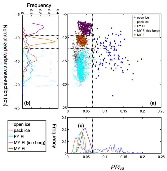
Figure 5.
(a) Scatterplot of σ0 and PR36. Blue diamonds indicate open water and open ice, respectively. Brown dots indicate pack ice. Light blue circles indicate FY fast ice, and purple or orange squares indicate MY fast ice, including icebergs and MY fast ice, respectively. (b),)c) Histograms of σ0 and PR36, respectively. The dotted line shows the threshold of the ice classification algorithm.
Conversely, drift ice cannot be classified from fast ice because the distribution of σ0 overlaps with that of fast ice. However, it is possible to classify pack ice and open ice by the PR36 distribution, as shown in Figure 5c. Regions with a PR36 value of 0.07 or more were classified as open ice areas, and regions with PR36 value of less than 0.07 were classified as pack ice areas. However, the PR36 values of pack ice are distributed in the same region as the FY fast ice in Figure 5c. Furthermore, the σ0 value of pack ice is distributed in the same region as FY fast ice in Figure 5b. Therefore, classification was difficult between FY fast ice and pack ice. In this study, pack ice, together with FY fast ice, was classified as FY ice. Areas with a SIC of less than 15% were classified as open water. The threshold value of 15% is a typical threshold used when calculating sea ice extents.
4. Validity Testing of the Ice Classification Scheme
To verify the validity of the ice classification algorithm, the algorithm results were compared with visual observation data obtained from the icebreaker Shirase from 9 December 2013 to 4 January 2014, as shown in Figure 6a. Routine visual observations of sea ice and ocean conditions were performed once every hour from the ship’s bridge. Visual observations included the thickness of snow and ice, the sea ice concentration, and the presence of surface melting. Figure 6b,c shows a comparison of the results of ice classification using visual observation and satellite data. It is assumed that the results of each observation represent the sea ice and ocean conditions of the region in which the Shirase sailed within each hour. The results were consistent with the observations up to a measurement distance of 400 km. After 400 km, there was a difference between the visual observation data and the classification results of this study. The range between 400 and 600 km was classified as open water by visual observation, whereas the classification algorithm classified it as FY ice. From the track shown in Figure 6a, the ship sailed in a flaw polynya called “Otone-suiro”, which is located along a fast ice area south of 67° S. The resolution of the SIC used to determine the open water was 10 km. A typical Antarctic coastal polynya is 0–10 km in width [30]. Satellite observations can include not only the polynya, but also the ice at its sides, whereas visual observation focuses on a narrow area around the ship. Thus, methodological differences between the algorithm calculations and visual observations may have caused the difference in results.
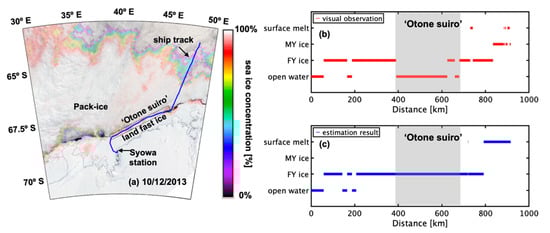
Figure 6.
(a) Track of the Japanese ice breaker Shirase from 9 December 2013 to 4 January 2014. (b,c) Comparison of sea ice classification by ship-based visual observations and by this classification algorithm.
The range between 800 and 850 km was classified as FY ice, and that after 850 km was classified as MY ice by visual observation (Figure 6b). The estimation results did not match the visual observation data after 800 km (Figure 6c). Visual observation determined melting when paddles (melting ponds) were observed on the surface. However, the melting algorithm detected not only the melting of the snow surfaces, but also the sub-surfaces. This difference in the determination of melting may have caused a discrepancy in the results between the two methods.
Table 2 shows an evaluation of the accuracy of in the proposed ice classification algorithm compared with the visual observation data. For example, the value of 43.3 in the open water row indicates that 43.3 km of the total of 111.8 km that was classified as open water by the algorithm was classified as FY ice by visual observation. The accuracy verification results examined three indices, which are generally used for satellite data verification, and these were calculated with reference to the calculation method of Hori et al. [31]. Here, producer’s accuracy (PA) indicates the accuracy ratio of the ice classification algorithm against visual observation. For example, 0.61 in the PA column was calculated from 68.5 divided by 111.8. User’s accuracy (UA) indicates the accuracy ratio of visual observation against the proposed ice classification algorithm. For example, 0.77 in the UA accuracy column was calculated from 68.5 divided by 88.9. Overall accuracy (OA) indicates the accuracy ratio of the distance in which the results of the proposed ice classification algorithm agree with those of visual observation against total distance. The values in parentheses are the results including the “Otone-suiro” polynya. The value of OA was 0.53 when including “Otone-suiro”, but increased to 0.71 when the polynya was excluded. As mentioned above, the “Otone-suiro” polynya was too narrow to be treated by the proposed ice classification algorithm. It is reasonable to evaluate this algorithm with observational data excluding “Otone-Suiro”. Additionally, visual observation can only detect surface melting; however, this ice classification algorithm can detect surface and subsurface melting covering a wide range of melting conditions. Except for the “Otone-Suiro” polynya and surface melting, the classification results showed a high level of agreement with the visual observation data. Thus, we concluded that the proposed algorithm performed well.
Table 2.
Error matrix of comparison between visual observation and the ice classification algorithm. The vertical columns show the ice classification results, while the horizontal rows show the results of visual observation as reference data. The accuracy was verified with the indicators of overall accuracy (OA), producer’s accuracy (PA), and user’s accuracy (UA). The values of PA, OA, and UA represent the ratios of accuracy, and other values represent the distances in km. The values in parentheses are the results including the “Otone-Suiro” polynya.
Figure 7a,d shows the MODIS images and Figure 7b,e shows C-SAR images for October 2015 and 2016, respectively. Figure 7c,f shows the results of the proposed ice classification algorithm. Here, the C-SAR images have lines on the edges of the ice shelf, MY ice, and the outer part of the ice tongue, respectively. These lines along the edges of different ice types were defined by analyzing the intensity of reflectance derived from the C-SAR images. Figure 7a–c indicate the season before the large ice breakup, and Figure 7d–f indicate the season after the large ice breakup. From the MODIS images shown in Figure 7a,d, it can be seen that drift ice and land fast ice were separated by flaw polynya, whereas ice types including FY ice, MY ice, ice shelf or ice sheets cannot be distinguished in the south of the flaw polynya. However, these ice types, except FY ice, could be classified by the C-SAR images shown in Figure 7b,e as mentioned above. The ice classification algorithm developed in this study was designed to classify these ice types, which are detected by MODIS and C-SAR, and the results are shown in Figure 7c,f. From Figure 7c, open ice at two offshore regions (33–35° E, 68.3–68.8° S and 38–43° E, 67.5–68.5° S) classified by the proposed algorithm corresponded to open water and newly formed ice, which appeared in the MODIS image at the boundary between drift ice and land fast ice, as shown in Figure 7a. Although the MODIS image shown in Figure 7d cannot distinguish between ice shelves and MY ice, the results of the ice classification algorithm shown in Figure 7f are in accordance with the edge of the ice shelf shown in Figure 7e. Moreover, the MY ice floe at 41.5–42.0° E, 68° S, shown in Figure 7e, was also confirmed. The C-SAR image shown in Figure 7b contained a square-shaped projection of ice shelf at the point indicated by A (38° E, 69.5° S) in 2015. This part of the ice shelf at A in 2015 was broken up in 2016. This change in ice shelf can also be confirmed from the classification results by the algorithm (Figure 7c,f). A MY ice outflow was confirmed around this ice shelf. In the open water, caused by breakup, the area of FY ice grew. This change in ice types was also confirmed by the ice classification algorithm results shown in Figure 7f. At the point indicated by B (35–37° E, 69° S) the breakup and separation of the ice shelf occurred, and many icebergs appeared. These events were confirmed from the C-SAR images. These ice type changes were also confirmed from the ice classification algorithm shown in Figure 7f as a change from an ice shelf to MY (IB) ice. The classification results also indicated that MY (IB) ice appeared at the boundary between the MY ice and the ice shelf.
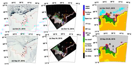
Figure 7.
Comparison of the ice classification images (a,d), MODIS imagery (b,e), and C-SAR imagery (c,f) for Lützow-Holm Bay. The lines shown in the C-SAR images indicate the edges of the MY fast ice, ice shelf, and the glacier.
Figure 8 shows the classification results of ice types and an enlarged image of the C-SAR image around the SG ice tongue. Here, the C-SAR images have lines tracing the outline of the ice shelf (green line) and the ice tongue (blue line), respectively. These lines along the edges of different ice types were defined by analyzing the intensity of reflectance derived from the C-SAR images. In 2017, the tip of the SG tongue flowed out as shown in Figure 8b. According to the classification results shown in Figure 8c,d, the ice in location 5 was classified as an ice shelf before breakup, while it was classified as a MY ice after breakup. The shape of the SG ice tongue changed after breakup, as shown by blue lines in Figure 8a,b. The results of the ice classification algorithm shown in Figure 8c,d show good agreement with these blue lines. The calculation results also show that the ice conditions at sea substantially changed after the breakup. A C-SAR image on 5 May 2017 confirmed that new ice started growing in location 5. Therefore, the ice shown in Figure 8b, which was only 1 month after the breakup event, appears to be FY ice. However, the algorithm classified the ice as MY ice because the value of σ0 was within the range of MY fast ice, as shown in Figure 2e. This discrepancy can be explained as follows. It has been reported that the salinity of the sea surface at the glacier edge is lower due to the presence of fresh water from the bottom of the glacier in Greenland [32,33]. Thus, ice formed from low-salinity sea water has lower dielectric loss and a higher σ0 value than ordinary FY ice. A similar effect of low-salinity water from the tip of the ice tongue was likely to have occurred at location 5.
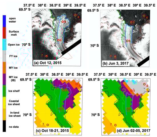
Figure 8.
Enlarged view around the ice tongue of Shirase Glacier. (a,c) Classification results and C-SAR images before outflow in April 2017. (b,d) Classification results and C-SAR images after outflow in May 2017.
5. Time Series Change in Ice Area
Figure 9 shows the inter-annual changes of the monthly averaged ice area in October for (a) the ice shelf, (b) MY and MY (IB) ice, and (c) FY ice, classified using the ice classification algorithm during the period of 2012 to 2018 in the region of 32–44° E and 67–71° S, including LHB. Hereafter, MY ice and MY (IB) ice are referred to as MY ice for simplicity.
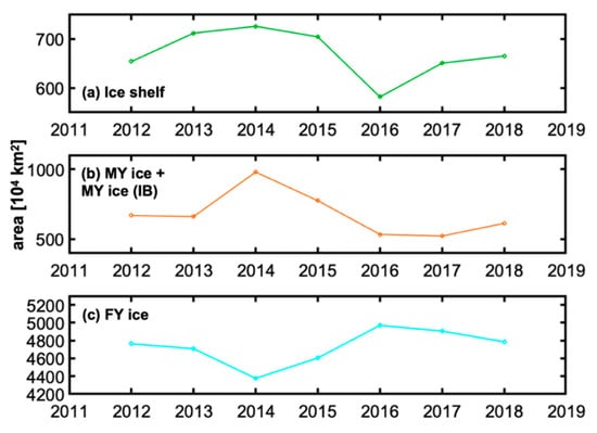
Figure 9.
Time series of (a) the ice shelf, (b) MY and MY (IB) ice, and (c) FY ice derived from the classification algorithm in October during the period of 2012 to 2018 in the region of Lützow-Holm Bay (32–44° E, 67–71° S).
The area of the ice shelf gradually increased and showed the largest area in 2014. The area then decreased until 2016, then recovering after that. The MY ice area was also largest in 2014, as was the ice shelf area. Conversely, the area of MY ice rapidly increased from 2013 to 2014, then continuously decreased from 2015 to 2016, exhibiting the smallest area in 2017.
As mentioned above, the areas of the ice shelf and MY ice had decreased during 2014 to 2016. However, there was a difference in the areal decrease. We focused on the ice edge to further study this difference. Figure 10 shows the ice edge of (a) the ice shelf and (b) MY ice, derived from the ice classification algorithm in October from 2013 to 2017.
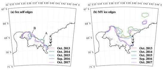
Figure 10.
The ice edge of (a) the ice shelf and (b) MY ice in Lützow-Holm Bay derived from the ice classification algorithm. Bold black lines show the coastline.
The MY ice exhibited seaward extension in two regions, namely 37–38° E, 68.5–69° S and 39–41° E, 68.5–69° S during 2013 to 2014. In 2015, the seaward extension retreated to return to the ice edge location at 39–41° E, 68.5–69° S in 2013. In 2016, a large ice breakup occurred in the MY ice and the ice edge retreated to a similar position as the ice shelf and did not recover until 2017. The breakup of the ice shelf occurred at A after a large breakup of MY ice in April 2016. Moreover, the breakup occurred not only at A but also in the western part of A shown in Figure 10a. However, the breakup of the ice shelf had not occurred until the large breakup in April 2016. As mentioned above, we considered the causes to indicate a difference in the areal decrease in these ice types. The large ice breakup of MY ice and the ice shelf in 2016 can be explained by this process, with the breakup of MY ice inducing the breakup of the ice shelf. This process was confirmed by the MODIS images from mid-March to early-April.
Figure 9 shows that the area of FY ice exhibited a mirrored pattern of MY ice, i.e., when the MY ice area was large, the FY ice area was small, and vice versa. This pattern can be seen in Figure 11 from a different perspective. The figure shows a comparison of the areas of FY ice and MY ice. There was a negative correlation between these ice types. Based on this relationship, it may be possible to show that MY ice was replaced by FY ice when ice breakup occurred. Conversely, FY ice developed into MY ice and extended seaward until an ice breakup event. Periodic breakups have been reported in LHB from 1980 to 2004 [17], and such ice breakups were reflected in the results of the current study. Importantly, the proposed ice classification algorithm was proven to be able to detect ice breakup events as quantitative changes in the distribution and ice type in a given area.
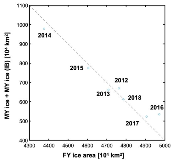
Figure 11.
Scatter plot for the FY ice and MY and MY (IB) ice around Lützow-Holm Bay (67–71° S, 32–44° E).
6. Conclusions
In the current study, we have investigated the annual changes of σ0 at eight locations in LHB, East Antarctica, by classifying ice types using ASCAT data. These ice types were defined by MODIS and C-SAR imagery of coastal Antarctica in the vicinity of LHB. An ice classification algorithm was then developed based on the threshold values of various parameters calculated from the features of each ice type (e.g. open ice, FY ice, MY ice, MY (IB) ice, ice shelf, coastal ice sheet, inland ice sheet) as shown in Figure 4. These parameters included the melting index, XPR, PR36, calculated from the brightness temperature, and the SIC, derived from AMSR2 instrument.
The MODIS images were not able to detect ice due to cloudy skies or insufficient sunlight. However, ASCAT and C-SAR, whose measurement wavelength ranges are in the microwave range, were able to observe ice in such situations. C-SAR images have a high resolution; however, the satellites have 18-day sub-cycles. Conversely, ASCAT is superior in terms of the temporal resolution, because data are acquired once every 3–4 days. Although the resolution is not as high as that of C-SAR images, ASCAT is superior in terms of spatiotemporal resolution.
To verify the validity of the proposed ice classification algorithm, the algorithm results were compared with visual observation data obtained from an icebreaker. Except for polynya and areas with surface melting, the results of the classification algorithm agreed with the visual observation data. The results of ice classification before and after large-scale breakup in April 2016, were compared with the corresponding MODIS and C-SAR imagery. The distribution of the MY ice and the ice shelf estimated by this ice classification algorithm matched that discernible from the satellite imagery.
Inter-annual changes in the areal extent of FY ice, MY ice, and the ice shelf were investigated using the new ice classification algorithm developed in this study. This investigation of MY ice and ice shelf areas indicated that the breakup of MY ice induced a breakup of the ice shelf. The comparison of FY ice and MY ice areas showed the replacement of these ice types. Previous studies have reported periodic breakups in LHB between 1980 and 2004 [17], and such ice breakups were detected in the current results. Importantly, the proposed ice classification algorithm was able to detect ice breakup events as quantitative changes in the distribution and type of ice in a given area. From the above, the ice classification algorithm developed in this study can successfully simultaneously classify FY ice, MY ice, ice shelves, and ice sheets around the Antarctic continent, which has not been possible with conventional algorithms until now.
In future work, we plan to classify sea ice in other sea ice areas to test the application of the proposed algorithm throughout the Antarctic region. Accurate classification of sea ice types is important for estimating sea ice thickness. However, because there is currently no validated method for estimating sea ice thickness in the Antarctic region, the findings of the current research, derived using a newly proposed algorithm, have valuable implications.
Author Contributions
S.H. processed the data and wrote the manuscript with advice and guidance from K.T. and K.I. All authors have read and agreed to the published version of the manuscript.
Funding
This research received no external funding.
Acknowledgments
The AMSR2 brightness temperature and sea-ice concentration product was provided by Japan Aerospace Exploration Agency. Normalized radar cross-section data were obtained from the NASA sponsored Scatterometer Climate Record Pathfinder at Brigham Young University courtesy of David G. Long. We acknowledge the use of imagery from the NASA Worldview application https://worldview.earthdata.nasa.gov), which is part of the NASA Earth Observing System Data and Information System (EOSDIS). This study was supported by the JAXA Second Research Announcement on the Earth Observations. We thank Benjamin Knight, MSc., from Edanz Group (https://en-author-services.edanzgroup.com/ac) for editing a draft of this manuscript.
Conflicts of Interest
The authors declare no conflict of interest.
References
- Reid, P.; Stammerjohn, S.; Massom, R.; Scambos, T.; Lieser, J. The record 2013 Southern Hemisphere sea-ice extent maximum. Ann. Glaciol. 2015, 56, 99–106. [Google Scholar] [CrossRef]
- Turner, J.; Phillips, T.; Marshall, G.J.; Hosking, J.S.; Pope, J.O.; Bracegirdle, T.J.; Deb, P. Unprecedented springtime retreat of Antarctic sea ice in 2016. Geophys. Res. Lett. 2017, 44, 6868–6875. [Google Scholar] [CrossRef]
- Vaughan, D.G.; Comiso, J.C.; Allison, I.; Carrasco, J.; Kaser, G.; Kwok, R.; Mote, P.; Murray, T.; Paul, F.; Ren, J.; et al. Observations: Cryosphere. Clim. Chang. 2013, 2103, 317–382. [Google Scholar]
- Laxon, S.W.; Giles, K.A.; Ridout, A.L.; Wingham, D.J.; Willatt, R.; Cullen, R.; Kwok, R.; Schweiger, A.; Zhang, J.; Haas, C.; et al. CryoSat-2 estimates of Arctic sea ice thickness and volume. Geophys. Res. Lett. 2013, 40, 732–737. [Google Scholar] [CrossRef]
- Price, D.; Rack, W.; Haas, C.; Langhorne, P.J.; Marsh, O. Sea ice freeboard in McMurdo Sound, Antarctica, derived by surface-validated ICESat laser altimeter data. J. Geophys. Res. Ocean. 2013, 118, 3634–3650. [Google Scholar] [CrossRef]
- Fedotov, V.I.; Cherepanov, N.V.; Tyshko, K.P. Some features of the growth, structure and metamorphism of east antarctic landfast sea ice. Antarct. Sea Ice Phys. Process. Interact. Var. 1998, 74, 343–354. [Google Scholar] [CrossRef]
- Heil, P.; Fowler, C.W.; Lake, S.E. Antarctic sea-ice velocity as derived from SSM/I imagery. Ann. Glaciol. 2006, 44, 361–366. [Google Scholar] [CrossRef]
- Massom, R.A.; Scambos, T.A.; Bennetts, L.G.; Reid, P.; Squire, V.A.; Stammerjohn, S.E. Antarctic ice shelf disintegration triggered by sea ice loss and ocean swell. Nature 2018, 558, 383–389. [Google Scholar] [CrossRef]
- Tamura, T.; Ohshima, K.I.; Nihashi, S. Mapping of sea ice production for Antarctic coastal polynyas. Geophys. Res. Lett. 2008, 35. [Google Scholar] [CrossRef]
- Aulicino, G.; Fusco, G.; Kern, S.; Budillon, G. Estimation of Sea-Ice thickness in Ross and Weddel Seas from SSM/I Brightness Temperatures. IEEE Trans. Geosci. Remote Sens. 2014, 52, 4122–4140. [Google Scholar] [CrossRef]
- Drinkwater, M.R. Satellite microwave radar observations of Antarctic sea ice. In Analysis of SAR Data of the Polar Oceans; Springer: Berlin/Heidelberg, Germany, 1998; pp. 145–187. [Google Scholar]
- Haas, C. The seasonal cycle of ERS scatterometer signatures over perennial Antartic sea ice and associated surface ice properties and processes. Ann. Glaciol. 2001, 33, 69–73. [Google Scholar] [CrossRef][Green Version]
- Belmonte Rivas, M.; Verspeek, J.; Verhoef, A.; Stoffelen, A. Bayesian sea ice detection with the advanced scatterometer ASCAT. IEEE Trans. Geosci. Remote Sens. 2012, 50, 2649–2657. [Google Scholar] [CrossRef]
- Lindell, D.B.; Long, D.G. High-resolution soil moisture retrieval with ASCAT. IEEE Geosci. Remote Sens. Lett. 2016, 13, 972–976. [Google Scholar] [CrossRef]
- Sugimoto, F.; Tamura, T.; Shimoda, H.; Uto, S.; Simizu, D.; Tateyama, K.; Hoshino, S.; Ozeki, T.; Fukamachi, Y.; Ushio, S.; et al. Interannual variability in sea-ice thickness in the pack-ice zone off Lützow-Holm Bay, East Antarctica. Polar Sci. 2016, 10, 43–51. [Google Scholar] [CrossRef]
- JCOMM Expert Team on Sea Ice (2014) Sea-Ice Nomenclature: Snapshot of the WMO Sea Ice Nomenclature WMO No. 259, Volume 1—Terminology and Codes; Volume II—Illustrated Glossary and III—International System of Sea-Ice Symbols). WMO-JCOMM: Geneva, Switzerland; p. 121, (WMO-No. 259 (I-III)). Available online: http://hdl.handle.net/11329/328 (accessed on 5 August 2020).
- Ushio, S. Factors affecting fast-ice break-up frequency in Lützow-Holm Bay, Antarctica. Ann. Glaciol. 2006, 44, 177–182. [Google Scholar] [CrossRef]
- Aoki, S. Breakup of land-fast sea ice in Lützow-Holm Bay, East Antarctica, and its teleconnection to tropical Pacific sea surface temperatures. Geophys. Res. Lett. 2017, 44, 3219–3227. [Google Scholar] [CrossRef]
- Figa-Saldaña, J.; Wilson, J.J.W.; Attema, E.; Gelsthorpe, R.; Drinkwater, M.R.; Stoffelen, A. The advanced scatterometer (ascat) on the meteorological operational (MetOp) platform: A follow on for european wind scatterometers. Can. J. Remote Sens. 2002, 28, 404–412. [Google Scholar] [CrossRef]
- Mortin, J.; Howell, S.E.L.; Wang, L.; Derksen, C.; Svensson, G.; Graversen, R.G.; Schrøder, T.M. Extending the QuikSCAT record of seasonal melt–freeze transitions over Arctic sea ice using ASCAT. Remote Sens. Environ. 2014, 141, 214–230. [Google Scholar] [CrossRef]
- Early, D.S.; Long, D.G. Image reconstruction and enhanced resolution imaging from irregular samples. IEEE Trans. Geosci. Remote Sens. 2001, 39, 291–302. [Google Scholar] [CrossRef]
- Lindsley, R.D.; Long, D.G. Adapting the SIR algorithm to ASCAT. 2010 IEEE Int. Geosci. Remote Sens. Symp. 2010, 3402–3405. [Google Scholar] [CrossRef]
- Long, D.G.; Hardin, P.J.; Whiting, P.T. Resolution enhancement of spaceborne scatterometer data. IEEE Trans. Geosci. Remote Sens. 1993, 31, 700–715. [Google Scholar] [CrossRef]
- Ashcraft, I.; Long, D. Comparison of methods for melt detection over greenland using active and passive Microwave measurements. Int. J. Remote Sens. 2006, 27, 2469–2488. [Google Scholar] [CrossRef]
- Arndt, S.; Willmes, S.; Dierking, W.; Nicolaus, M. Timing and regional patterns of snowmelt on Antarctic sea ice from passive microwave satellite observations. J. Geophys. Res. Ocean. 2016, 121, 5916–5930. [Google Scholar] [CrossRef]
- Markus, T.; Burns, B.A. A method to estimate subpixel-scale coastal polynyas with satellite passive microwave data. J. Geophys. Res. Ocean. 1995, 100, 4473–4487. [Google Scholar] [CrossRef]
- Nihashi, S.; Ohshima, K.I.; Kimura, N. Creation of a heat and salt flux dataset associated with sea ice production and melting in the Sea of Okhotsk. J. Clim. 2012, 25, 2261–2278. [Google Scholar] [CrossRef]
- Winebrenner, D.P.; Nelson, E.D.; Colony, R.; West, R.D. Observation of melt onset on multiyear Arctic sea ice using the ERS 1 synthetic aperture radar. J. Geophys. Res. Ocean. 1994, 99, 22425–22441. [Google Scholar] [CrossRef]
- Kawamura, T.; Wakabayashi, H.; Ushio, S. Growth, properties and relation to radar backscatter coefficient of sea ice in Lützow-Holm Bay, Antarctica. Ann. Glaciol. 2006, 44, 163–169. [Google Scholar] [CrossRef][Green Version]
- Ishikawa, T.; Ukita, J.; Ohshima, K.I.; Wakatsuchi, M.; Yamanouchi, T.; Ono, N. Coastal polynyas off east queen maud land observed from NOAA AVHRR data. J. Oceanogr. 1996, 52, 389–398. [Google Scholar] [CrossRef]
- Hori, M.; Sugiura, K.; Kobayashi, K.; Aoki, T.; Tanikawa, T.; Kuchiki, K.; Niwano, M.; Enomoto, H. A 38-year (1978–2015) Northern Hemisphere daily snow cover extent product derived using consistent objective criteria from satellite-borne optical sensors. Remote Sens. Environ. 2017, 191, 402–418. [Google Scholar] [CrossRef]
- Meire, L.; Mortensen, J.; Meire, P.; Juul-Pedersen, T.; Sejr, M.K.; Rysgaard, S.; Nygaard, R.; Huybrechts, P.; Meysman, F.J. Marine-terminating glaciers sustain high productivity in Greenland fjords. Glob. Chang. Biol. 2017, 23, 5344–5357. [Google Scholar] [CrossRef]
- Kanna, N.; Sugiyama, S.; Ohashi, Y.; Sakakibara, D.; Fukamachi, Y.; Nomura, D. Upwelling of macronutrients and dissolved inorganic carbon by a subglacial freshwater driven plume in bowdoin fjord, northwestern greenland. J. Geophys. Res. Biogeosciences 2018, 123, 1666–1682. [Google Scholar] [CrossRef]
© 2020 by the authors. Licensee MDPI, Basel, Switzerland. This article is an open access article distributed under the terms and conditions of the Creative Commons Attribution (CC BY) license (http://creativecommons.org/licenses/by/4.0/).