Development of Fog Detection Algorithm Using GK2A/AMI and Ground Data


Abstract
1. Introduction
2. Materials and Methods
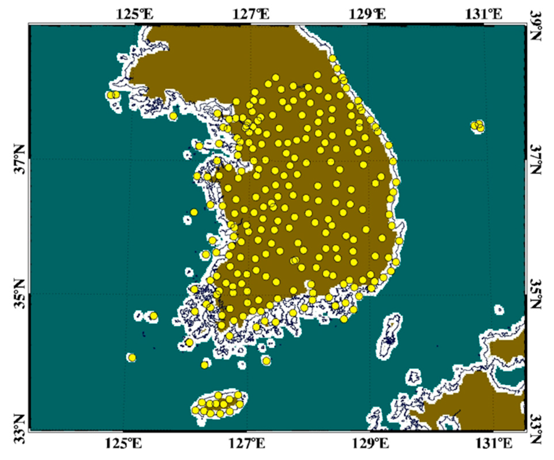
2.1. Materials
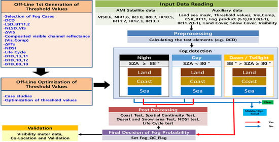
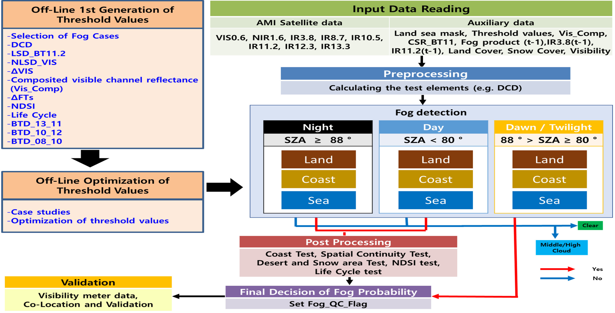
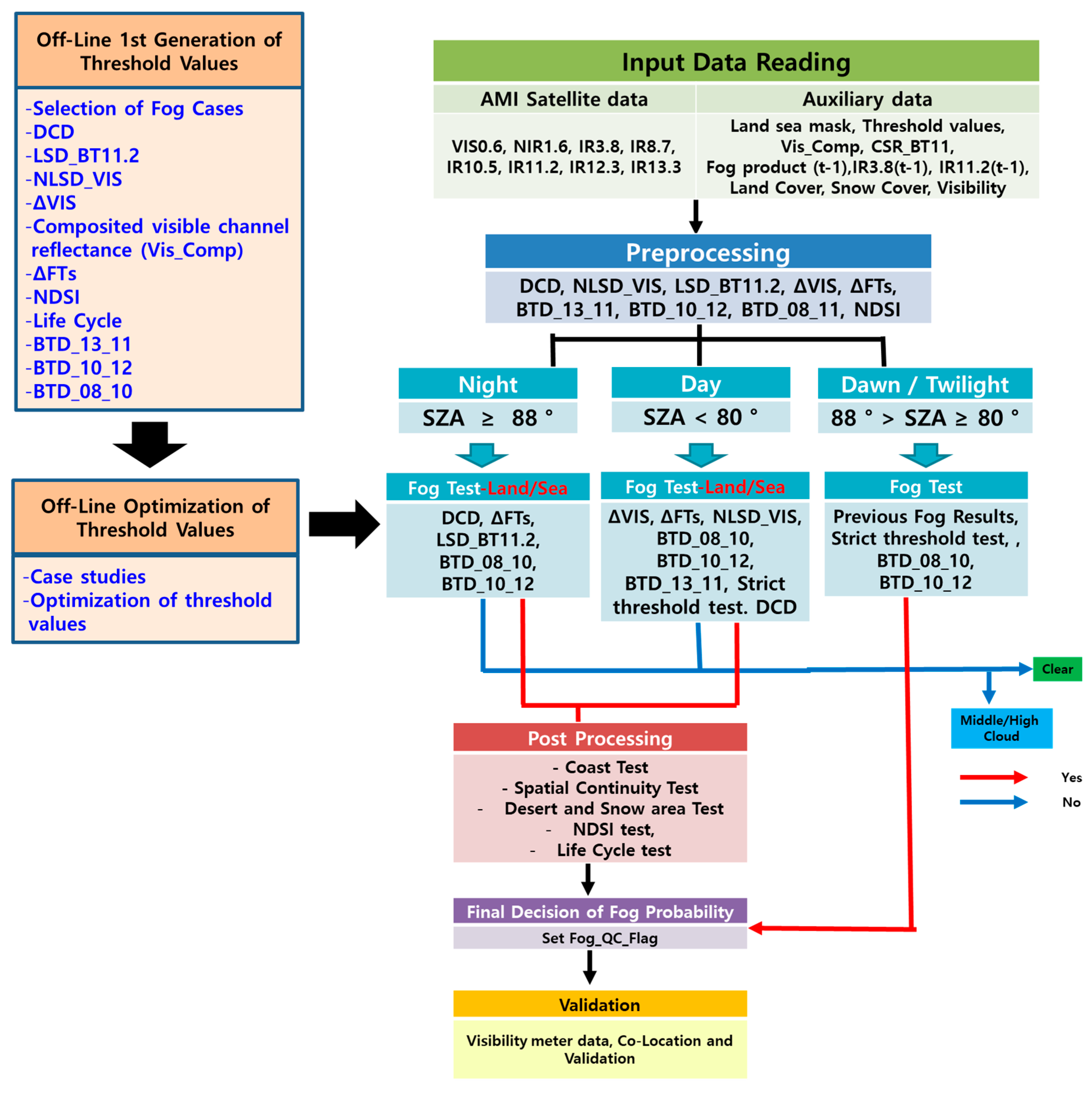
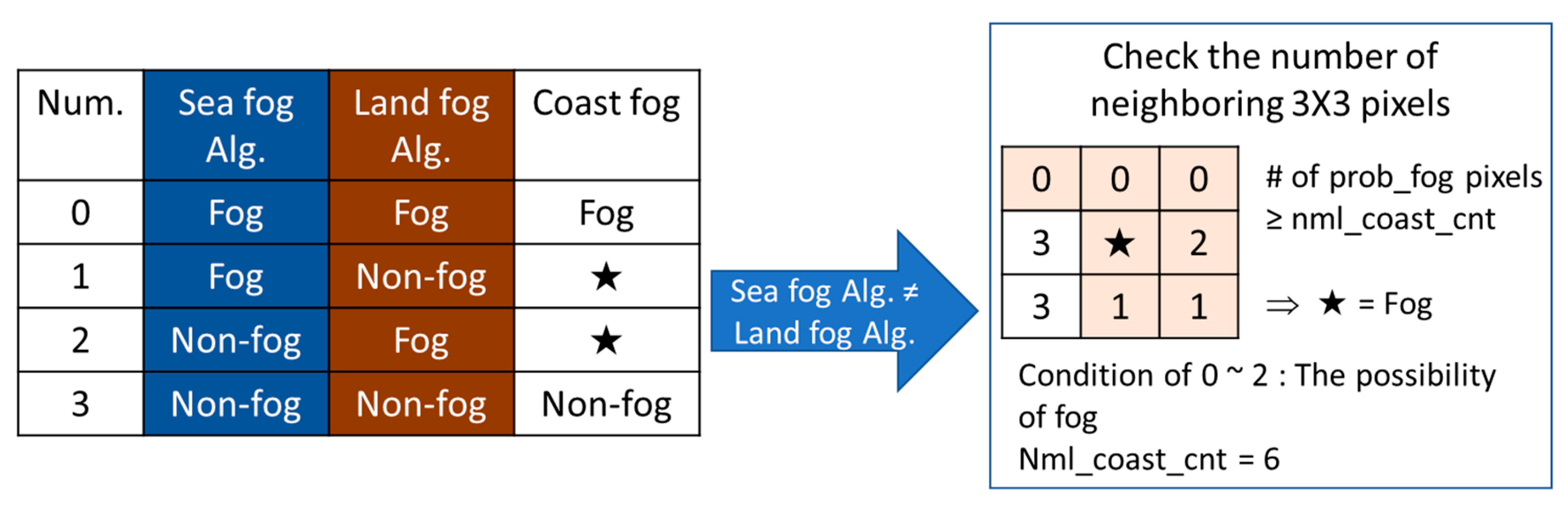
2.2. Methods
3. Results
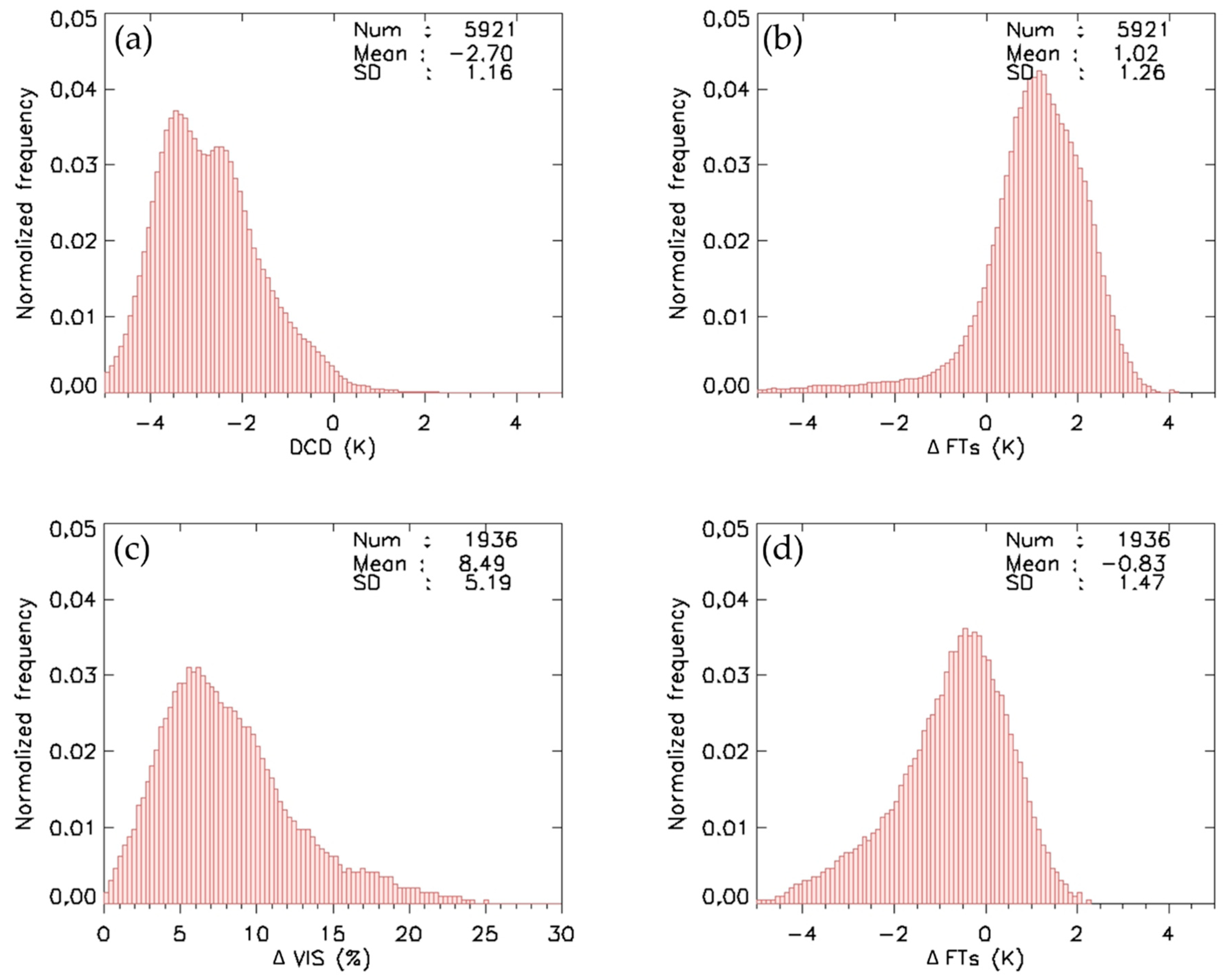
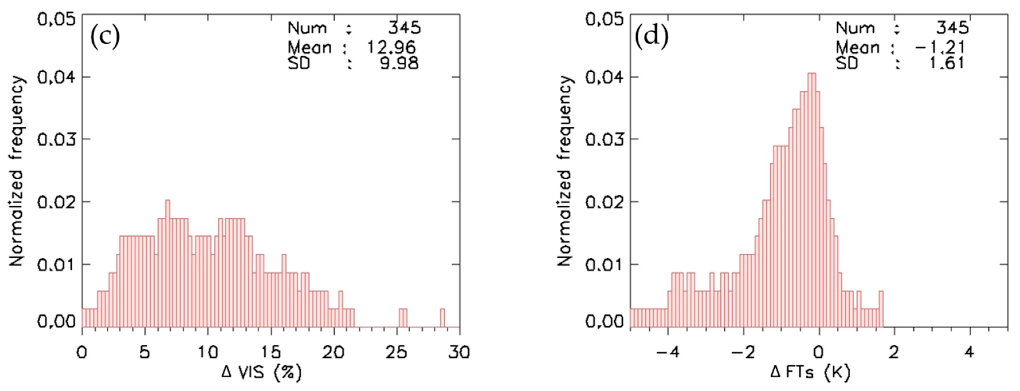
3.1. Frequency Analysis for Setting Threshold Values
3.2. Validation Results of Fog Detection Algorithm
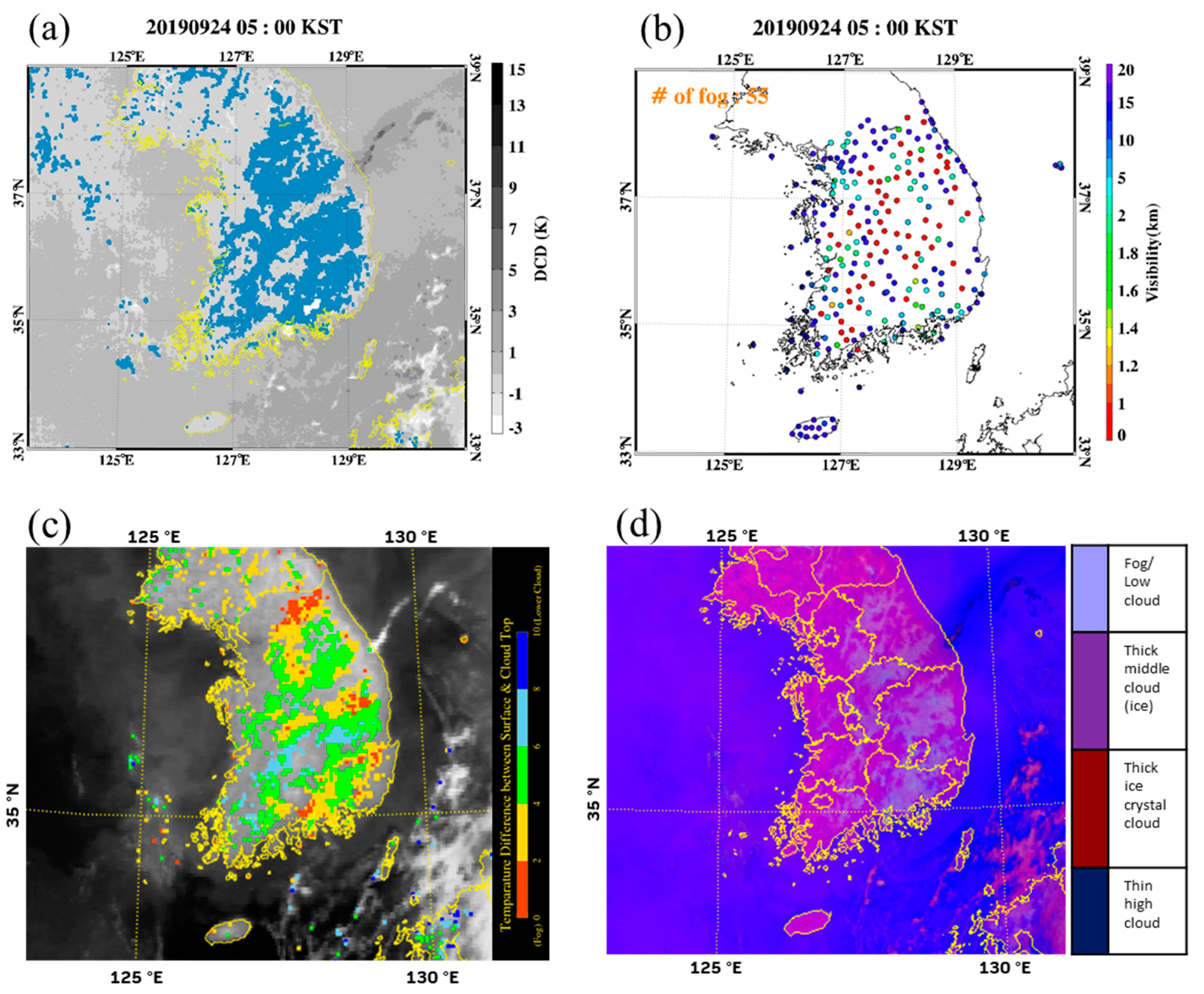
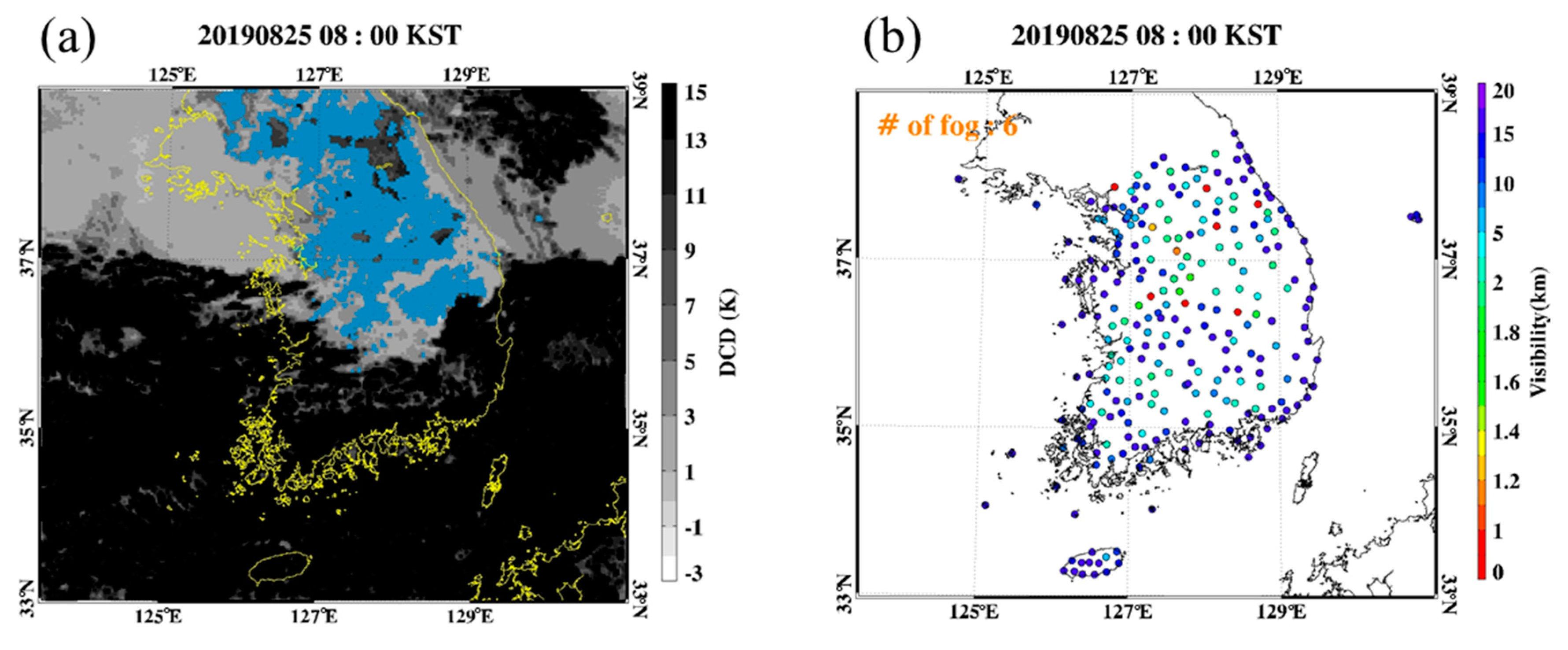
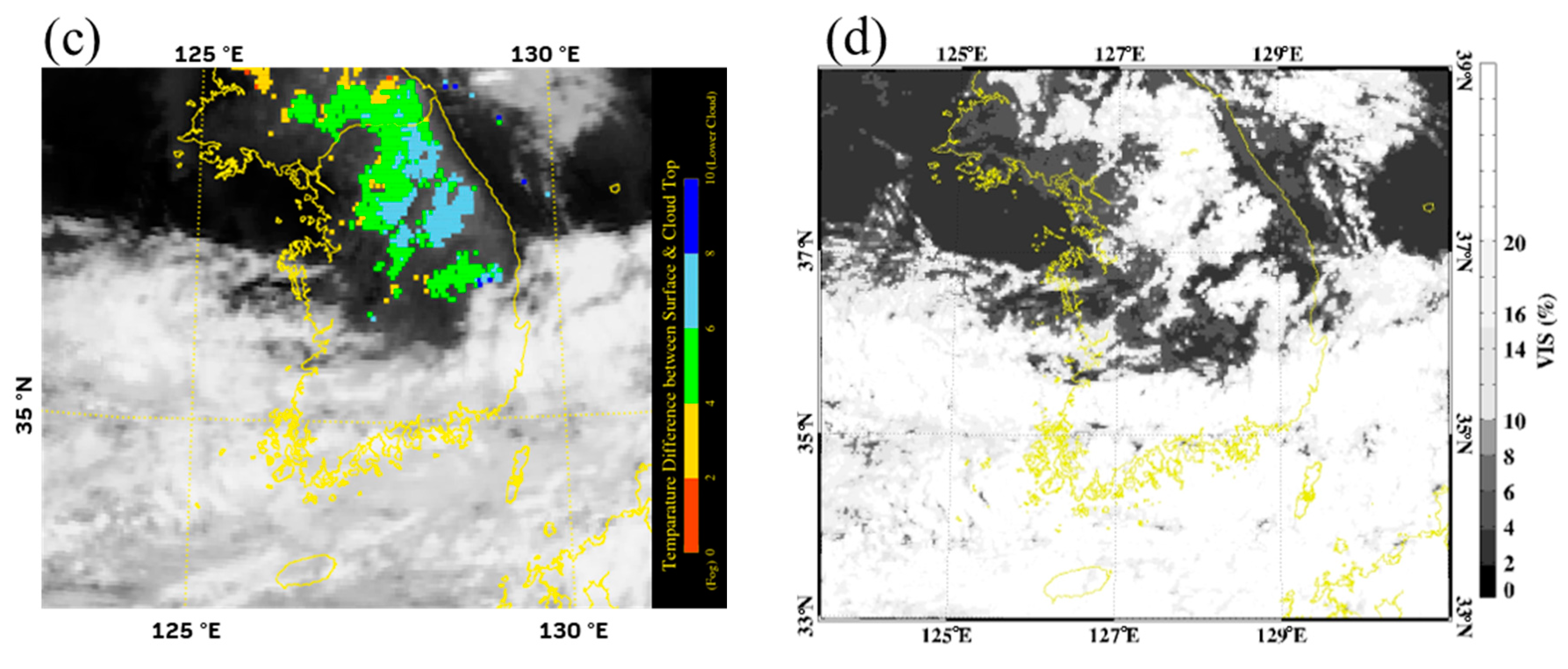
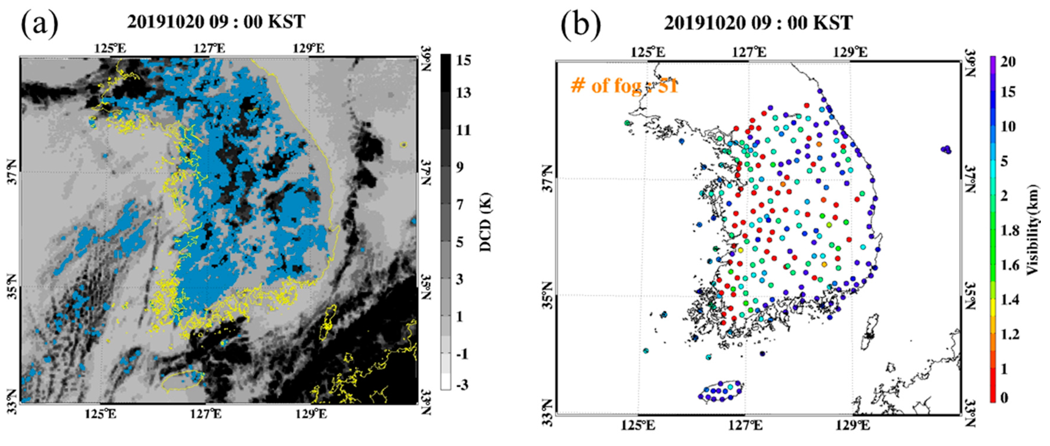
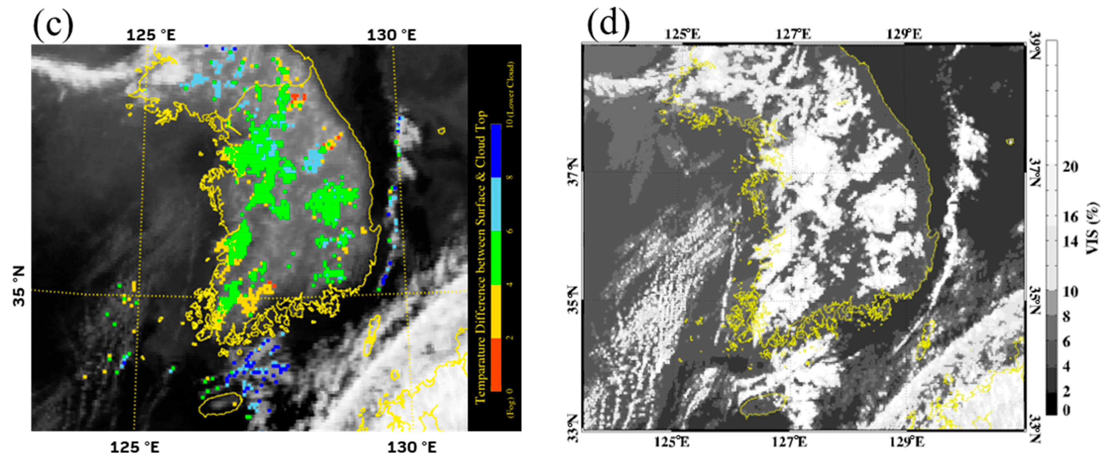
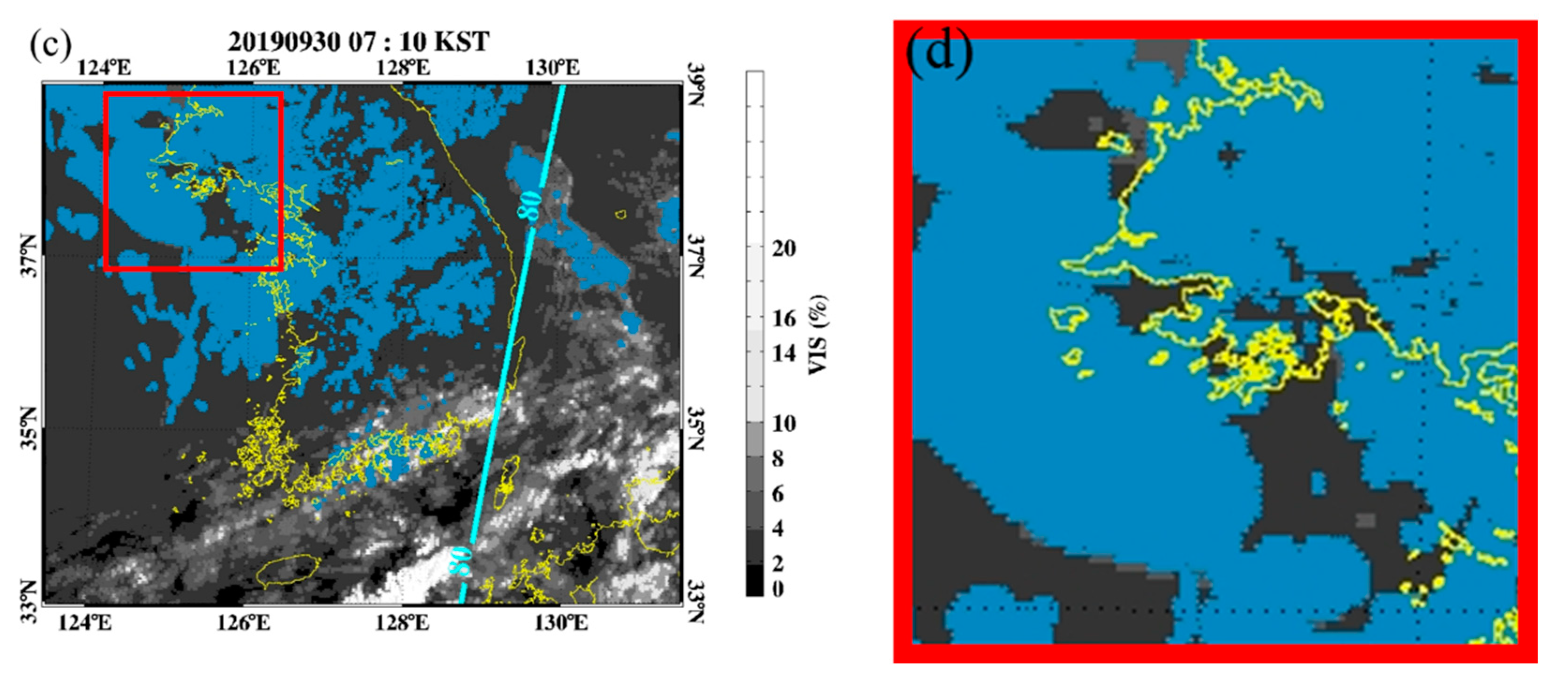
3.2.1. Fog Detection Results
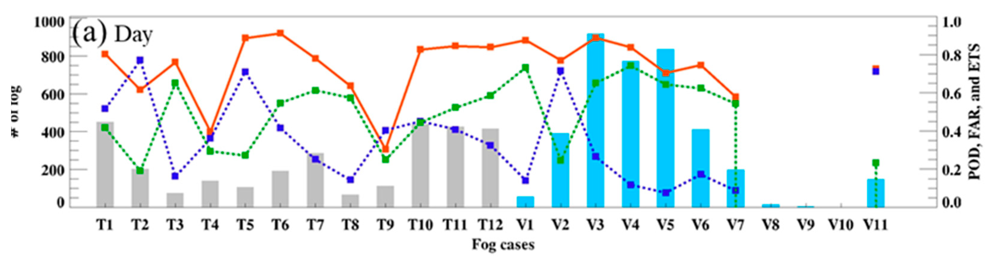
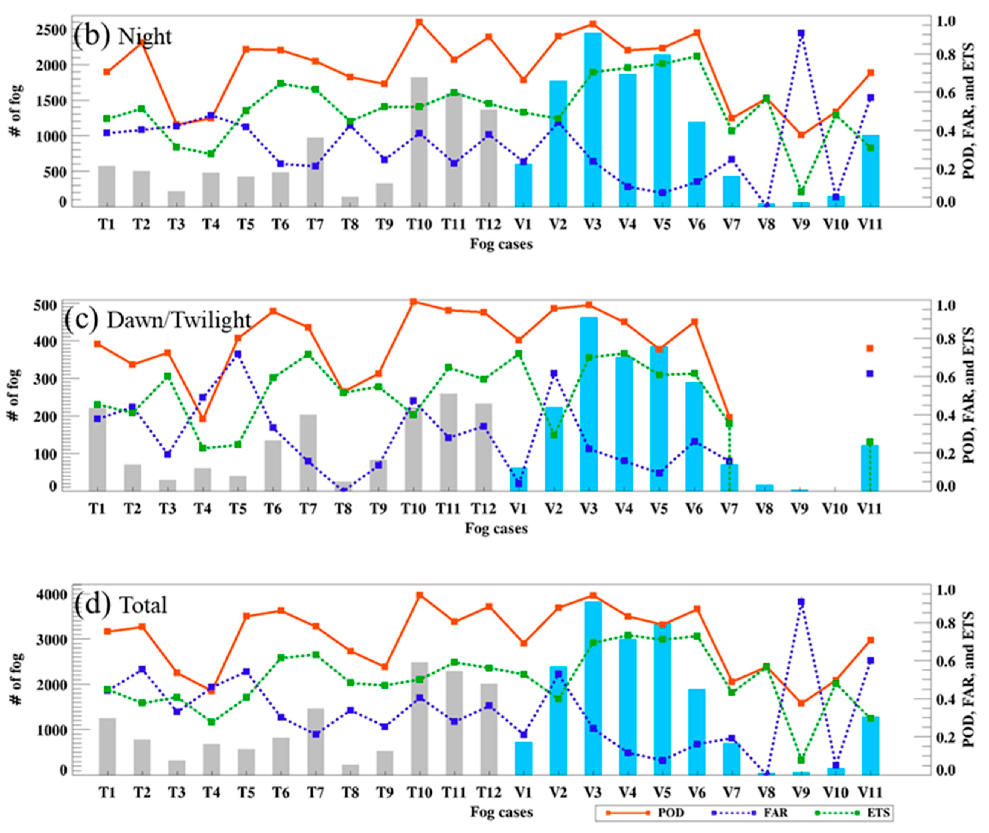
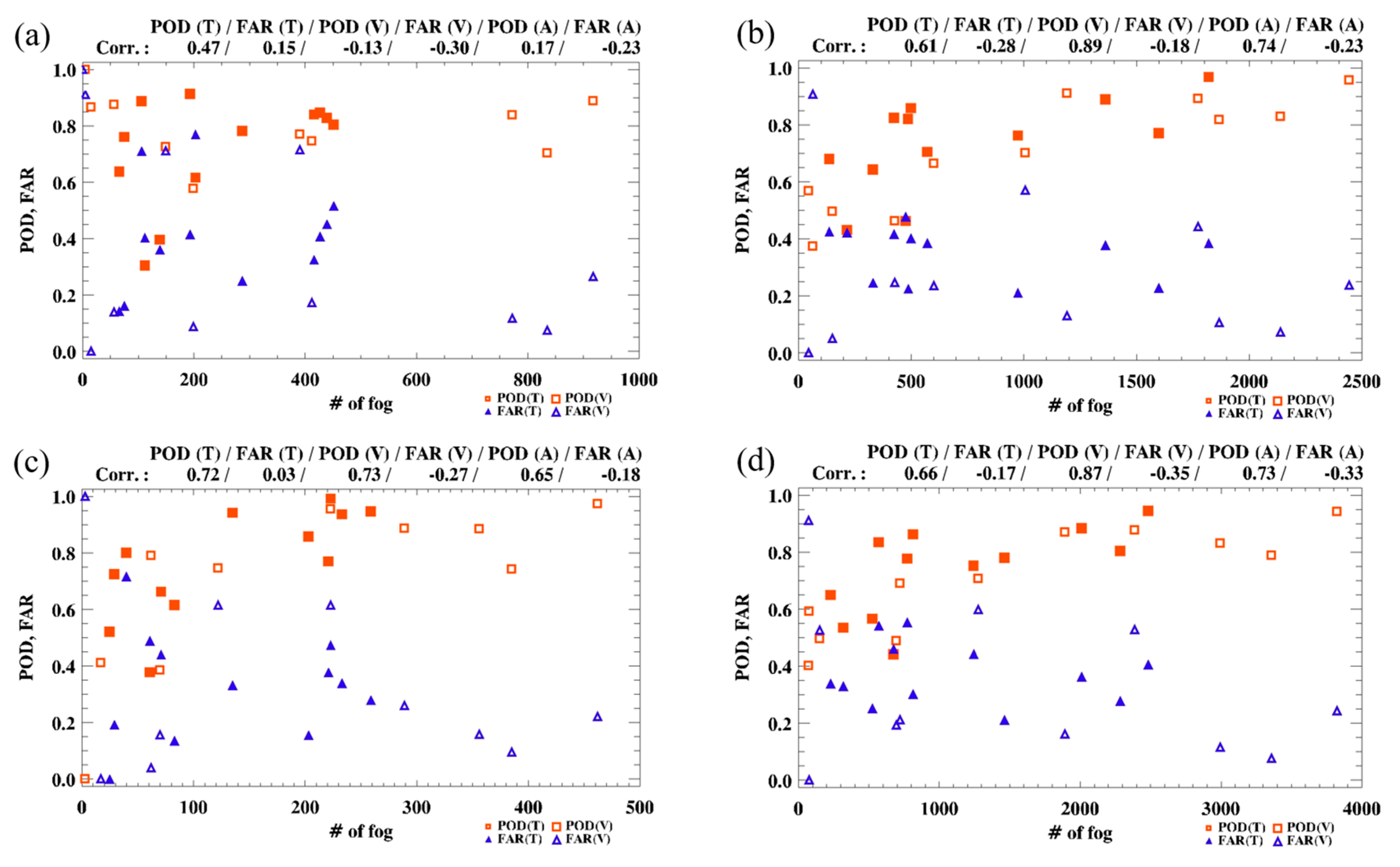
3.2.2. Quantitative Validation Results
4. Discussion
5. Conclusions
Author Contributions
Funding
Acknowledgments
Conflicts of Interest
Appendix A. Test Elements and Acronyms

| Test Elements | Unit | Definition |
|---|---|---|
| DCD | K | BT3.8 − BT11.2 |
| ΔVIS | % | VIS0.6 − Vis_Comp. |
| Vis_Comp | % | minimum value composite of visible channel reflectance during 30 days |
| ΔFTs | K | BT11.2 − CSR_BT11 |
| LSD | K | Standard deviation of 3 × 3 pixels |
| NLSD | LSD/Average of 3 × 3 pixels | |
| BTD_08_10 | K | BT8.7 − BT10.5 |
| BTD_10_12 | K | BT10.5 − BT12.3 |
| BTD_13_11 | K | BT13.3 − BT11.2 |
| Acronyms | Description |
|---|---|
| ABI | Advanced Baseline Imager |
| AHI | Advanced Himawari Imager |
| AMI | Advanced Meteorological Imager |
| ASOS | Automated Surface Observing System |
| AWOS | Automated Weather Observing System |
| Bias | Bias Ratio |
| BT | Brightness Temperature |
| BTD | Brightness Temperature Difference |
| CALIPSO | Cloud-Aerosol Lidar and Infrared Pathfinder Satellite Observation |
| COMS | Communication, Ocean and Meteorological Satellite |
| Corr. | Correlation coefficients |
| CMDPS | COMS Meteorological Data Processing System |
| CSR | Clear Sky Radiance |
| CSR_BT11 | Clear sky radiance for brightness temperature at 11 µm |
| DCD | Dual Channel Difference |
| ETS | Equitable Threat Score |
| FAR | False Alarm Ratio |
| ΔFTs | Difference between the BT of the fog top and surface temperature |
| GK2A | GEO-KOMPSAT-2A |
| GK2A_FDA | Fog detection algorithm of GK2A |
| GOES | Geostationary Operational Environmental Satellite |
| ISAI | Infrared Atmospheric Sounding Interferometer |
| IR | Infrared |
| KMA | Korea Meteorological Administration |
| KSS | Hanssen-Kuiper skill score |
| LSD | Local Standard Deviation |
| LSD_BT11.2 | LSD of Brightness Temperature at 11.2 μm |
| METAR | Meteorological Terminal Aviation Routine Weather Report |
| MTSAT | Multifunction Transport Satellite |
| NDSI | Normalized Difference Snow Index |
| NIR | Near Infrared |
| NLSD | Normalized LSD |
| NLSD_vis | NLSD of reflectance |
| NMSC | National Meteorological Satellite Center |
| NWP | Numerical Weather Model |
| POD | Probability Of Detection |
| RGB | Red-Green-Blue |
| RTTOV | Radiative Transfer of TOVS |
| SD | Standard Deviation |
| SEVIRI | Spinning Enhanced Visible and Infrared Imager |
| SYNOP | Surface Synoptic Observations |
| SZA | Solar Zenith Angle |
| UM | Unified Model |
| VFM | Vertical Feature Mask |
| VIS | Visible |
| ΔVIS | Difference between the reflectance of 0.64 μm (VIS0.6) and Vis_Comp |
| Vis_Comp | minimum value composite of visible channel reflectance during 30 days |
References
- Cermak, J. SOFOS—A New Satellite-Based Operational fog Observation Scheme. Ph.D. Thesis, Phillipps-University, Marburg, Germany, 2006. [Google Scholar] [CrossRef]
- Suh, M.S.; Lee, S.J.; Kim, S.H.; Han, J.H.; Seo, E.K. Development of Land fog Detection Algorithm based on the Optical and Textural Properties of Fog using COMS Data. Korean J. Remote Sens. 2017, 33, 359–375. [Google Scholar] [CrossRef]
- Han, J.H.; Suh, M.S.; Kim, S.H. Development of Day Fog Detection Algorithm Based on the Optical and Textural Characteristics Using Himawari-8 Data. Korean J. Remote Sens. 2019, 35, 117–136. [Google Scholar] [CrossRef]
- Bendix, J. A satellite-based climatology of fog and low-level stratus in Germany and adjacent areas. Atmos. Res. 2002, 64, 3–18. [Google Scholar] [CrossRef]
- Yi, L.; Thies, B.; Zhang, S.; Shi, X.; Bendix, J. Optical thickness and effective radius retrievals of low stratus and fog from MTSAT daytime data as a prerequisite for Yellow Sea fog detection. Remote Sens. 2015, 8, 8. [Google Scholar] [CrossRef]
- Ellrod, G.P. Advances in the detection and analysis of fog at night using GOES multispectral infrared imagery. Weather Forecast. 1995, 10, 606–619. [Google Scholar] [CrossRef]
- Jhun, J.G.; Lee, E.J.; Ryu, S.A.; Yoo, S.H. Characteristics of regional fog occurrence and its relation to concentration of air pollutants in South Korea. Atmosphere 1998, 23, 103–112. [Google Scholar]
- Underwood, S.J.; Ellrod, G.P.; Kuhnert, A.L. A multiple-case analysis of nocturnal radiation-fog development in the central valley of California utilizing the GOES nighttime fog product. J. Appl. Meteorol. 2004, 43, 297–311. [Google Scholar] [CrossRef]
- Heo, K.Y.; Ha, K.J. Classification of synoptic pattern associated with coastal fog around the Korean peninsula. Atmosphere 2004, 40, 541–556. [Google Scholar]
- Gultepe, I.; Müller, M.D.; Boybeyi, Z. A new visibility parameterization for warm-fog applications in numerical weather prediction models. J. Appl. Meteorol. Climatol. 2006, 45, 1469–1480. [Google Scholar] [CrossRef]
- Van der Velde, I.R.; Steeneveld, G.J.; Wichers Schreur, B.G.J.; Holtslag, A.A.M. Modeling and forecasting the onset and duration of severe radiation fog under frost conditions. Mon. Weather Rev. 2010, 138, 4237–4253. [Google Scholar] [CrossRef]
- Lee, H.D.; Ahn, J.B. Study on classification of fog type based on its generation mechanism and fog predictability using empirical method. Atmosphere 2013, 23, 103–112. [Google Scholar] [CrossRef]
- Musial, J.P.; Hüsler, F.; Sütterlin, M.; Neuhaus, C.; Wunderle, S. Daytime low stratiform cloud detection on AVHRR imagery. Remote Sens. 2014, 6, 5124–5150. [Google Scholar] [CrossRef]
- Lee, J.R.; Chung, C.Y.; Ou, M.L. Fog detection using geostationary satellite data: Temporally continuous algorithm. Asia Pac. J. Atmos. Sci. 2011, 47, 113–122. [Google Scholar] [CrossRef]
- Shin, D.; Kim, J.H. A new application of unsupervised learning to nighttime sea fog detection. Asia Pac. J. Atmos. Sci. 2018, 54, 527–544. [Google Scholar] [CrossRef]
- Shin, D.G.; Park, H.M.; Kim, J.H. Analysis of the Fog Detection Algorithm of DCD Method with SST and CALIPSO Data. Atmosphere 2013, 23, 471–483. [Google Scholar] [CrossRef]
- Ishida, H.; Miura, K.; Matsuda, T.; Ogawara, K.; Goto, A.; Matsuura, K.; Sato, Y.; Nakajima, T.Y. Scheme for detection of low clouds from geostationary weather satellite imagery. Atmos. Res. 2014, 143, 250–264. [Google Scholar] [CrossRef]
- Egli, S.; Thies, B.; Bendix, J. A hybrid approach for fog retrieval based on a combination of satellite and ground truth data. Remote Sens. 2018, 10, 628. [Google Scholar] [CrossRef]
- Eyre, J.R.; Brownscombe, J.L.; Allam, R.J. Detection of fog at night using advanced very high resolution radiometer (AVHRR) imagery. Meteorol. Mag. 1984, 113, 266–271. [Google Scholar]
- Kim, S.H.; Suh, M.S.; Han, J.H. Development of Fog Detection Algorithm during Nighttime Using Himawari-8/AHI Satellite and Ground Observation Data. Asia Pac. J. Atmos. Sci. 2019, 55, 337–350. [Google Scholar] [CrossRef]
- Cermak, J. Fog and low cloud frequency and properties from active-sensor satellite data. Remote Sens. 2018, 10, 1209. [Google Scholar] [CrossRef]
- Ellrod, G.P.; Gultepe, I. Inferring low cloud base heights at night for aviation using satellite infrared and surface temperature data. Pure Appl. Geophys. 2007, 164, 1193–1205. [Google Scholar] [CrossRef]
- Park, H.M.; Kim, J.H. Detection of sea fog by combining MTSAT infrared and AMSR microwave measurements around the Korean Peninsula. Atmosphere 2012, 22, 163–174. [Google Scholar] [CrossRef]
- Cermak, J.; Bendix, J. A novel approach to fog/low stratus detection using Meteosat 8 data. Atmos. Res. 2008, 87, 279–292. [Google Scholar] [CrossRef]
- Jeon, J.Y.; Kim, S.H.; Yang, C.S. Fundamental research on spring season daytime sea fog detection using MODIS in the yellow sea. Korean J. Remote Sens. 2016, 32, 339–351. [Google Scholar] [CrossRef]
- Choi, Y.S.; Ho, C.H. Earth and environmental remote sensing community in South Korea: A review. Remote Sens. Appl. Soc. Environ. 2015, 2, 66–76. [Google Scholar] [CrossRef]
- Chung, S.R.; Ahn, M.H.; Han, K.S.; Lee, K.T.; Shin, D.B. Meteorological Products of Geo-KOMPSAT 2A (GK2A) Satellite. Asia Pac. J. Atmos. Sci. 2020, 56, 185. [Google Scholar] [CrossRef]
- EUMETSAT. Best Practices for RGB Compositing of Multi-Spectral Imagery; User Service Division, EUMETSAT: Darmstadt, Germany, 2009; p. 8. [Google Scholar]
- Cermak, J. Low clouds and fog along the South-Western African coast—Satellite-based retrieval and spatial patterns. Atmos. Res. 2012, 116, 15–21. [Google Scholar] [CrossRef]
- NMSC. Cloud Mask Algorithm Theoretical Basis Document. Available online: http://nmsc.kma.go.kr/homepage/html/base/cmm/selectPage.do?page=static.edu.atbdGk2a (accessed on 2 July 2020).
- King, M.D.; Kaufman, Y.J.; Menzel, W.P.; Tanre, D. Remote sensing of cloud, aerosol, and water vapor properties from the moderate resolution imaging spectrometer(MODIS). IEEE Trans. Geosci. Remote Sens. 1992, 30, 2–27. [Google Scholar] [CrossRef]
- Baum, B.A.; Platnick, S. Introduction to MODIS cloud products. In Earth Science Satellite Remote Sensing, 1st ed.; Qu, J.J., Gao, W., Kafatos, M., Murphy, R.E., Salomonson, V.V., Eds.; Springer: Berlin/Heidelberg, 2006; Volume 1, pp. 74–91. [Google Scholar]
- Lee, H.K.; Suh, M.S. Objective Classification of Fog Type and Analysis of Fog Characteristics Using Visibility Meter and Satellite Observation Data over South Korea. Atmosphere 2019, 29, 639–658. [Google Scholar] [CrossRef]
- Andersen, H.; Cermak, J. First fully diurnal fog and low cloud satellite detection reveals life cycle in the Namib. Atmos. Meas. Tech. 2018, 11. [Google Scholar] [CrossRef]
- Dong, C. Remote sensing, hydrological modeling and in situ observations in snow cover research: A review. J. Hydrol. 2018, 561, 573–583. [Google Scholar] [CrossRef]
- Schreiner, A.J.; Ackerman, S.A.; Baum, B.A.; Heidinger, A.K. A multispectral technique for detecting low-level cloudiness near sunrise. J. Atmos. Ocean Technol. 2007, 24, 1800–1810. [Google Scholar] [CrossRef]
- Lefran, D. A One-Year Geostationary Satellite-Derived Fog Climatology for Florida. Master’s Thesis, Florida State University, Tallahassee, FL, USA, 2015. [Google Scholar]
- Nilo, S.T.; Romano, F.; Cermak, J.; Cimini, D.; Ricciardelli, E.; Cersosimo, A.; Paola, F.D.; Gallucci, D.; Gentile, S.; Geraldi, E.; et al. Fog detection based on meteosat second generation-spinning enhanced visible and infrared imager high resolution visible channel. Remote Sens. 2018, 10, 541. [Google Scholar] [CrossRef]
- Leppelt, T.; Asmus, J.; Hugershofer, K. Preliminary studies of MTG potential in satellite based fog and low cloud detection. In Proceedings of the 2018 EUMETSAT Meteorological Satellite Conference, Tallinn, Estonia, 17–21 September 2018. [Google Scholar]
- Wu, D.; Lu, B.; Zhang, T.; Yan, F. A method of detecting sea fogs using CALIOP data and its application to improve MODIS-based sea fog detection. J. Quant. Spectrosc. Radiat. Transf. 2015, 153, 88–94. [Google Scholar] [CrossRef]
- Kang, T.H.; Suh, M.S. Detailed Characteristics of Fog Occurrence in South Korea by Geographic Location and Season—Based on the Recent Three Years (2016–2018) Visibility Data. J. Clim. Res. 2019, 14, 221–244. [Google Scholar] [CrossRef]


| Channel | AMI Band | Wavelength | Spatial Resolution [km] | |
|---|---|---|---|---|
| (min) [µm] | (max) [µm] | |||
| 3 | VIS0.6 | 0.63 | 0.66 | 0.5 |
| 6 | NIR1.6 | 1.60 | 1.62 | 2 |
| 7 | IR3.8 | 3.74 | 3.96 | 2 |
| 11 | IR8.7 | 8.44 | 8.76 | 2 |
| 13 | IR10.5 | 10.25 | 10.61 | 2 |
| 14 | IR11.2 | 11.08 | 11.32 | 2 |
| 15 | IR12.3 | 12.15 | 12.45 | 2 |
| 16 | IR13.3 | 13.21 | 13.39 | 2 |
| Training Cases | Validation Cases | ||||||
|---|---|---|---|---|---|---|---|
| Code | Date | # of Fog | # of Station | Code | Date | # of Fog | # of Station |
| T1 | 07.04.2019 | 1244 | 25,002 | V1 | 10.01.2019 | 719 | 4473 |
| T2 | 07.14.2019 | 774 | 23,339 | V2 | 10.04.2019 | 2385 | 30,800 |
| T3 | 07.24.2019 | 320 | 7604 | V3 | 10.20.2019 | 3823 | 37,224 |
| T4 | 07.26.2019 | 676 | 6523 | V4 | 11.05.2019 | 2995 | 37,627 |
| T5 | 08.25.2019 | 570 | 22,897 | V5 | 11.06.2019 | 3360 | 25,912 |
| T6 | 08.26.2019 | 815 | 20,239 | V6 | 11.12.2019 | 1893 | 26,556 |
| T7 | 08.30.2019 | 1464 | 33,869 | V7 | 12.08.2019 | 696 | 34,425 |
| T8 | 08.31.2019 | 227 | 25,412 | V8 | 12.19.2019 | 76 | 23,189 |
| T9 | 09.17.2019 | 525 | 29,818 | V9 | 02.10.2020 | 72 | 21,291 |
| T10 | 09.24.2019 | 2483 | 16,278 | V10 | 02.11.2020 | 151 | 19,368 |
| T11 | 09.29.2019 | 2286 | 33,642 | V11 | 03.01.2020 | 1277 | 15,523 |
| T12 | 09.30.2019 | 2011 | 30,075 | ||||
| Total | 13,395 | 274,698 | Total | 15,175 | 162,592 | ||
| Time | Step | Test Elements | Land | Sea |
|---|---|---|---|---|
| Day | 1 | ΔVIS [%] | 3.0 | 4.0 |
| 2 | ΔFTs [K] | −2.5 & 1.0 | −4.0 | |
| 3 | NLSD_vis | - | 0.30 | |
| 4 | BTD_08_10 [K] | −1.3 | - | |
| 5 | BTD_10_12 [K] | 4.0 | 4.0 −19.0 | |
| 6 | BTD_13_11 [K] | −19.0 | ||
| 7 | Strict threshold test (ΔVIS [%], ΔFTs[K], NLSD_vis) | 4.0, −4.0, 0.10 (used when SZA < 60°) | - | |
| 8 | DCD [K] | - | −1.0–23.0 (SZA: 80.0–20.0°) | |
| Night | 1 | DCD [K] | −1.25 | −0.5 |
| 2 | ΔFTs [K] | −0.5 | −4.0 | |
| 3 | LSD_BT11.2 | 2.0 | 1.0 | |
| 4 | BTD_08_10 [K] | −1.3 | - | |
| 5 | BTD_10_12 [K] | 4.0 | 4.0 | |
| Dawn | 1 | Strict threshold test (DCD [K], ΔFTs [K], LSD_BT11.2 [K]) | −1.9, −5.0, 0.8 | - |
| 2 | BTD_08_10 [K] | −1.3 | - | |
| 3 | BTD_10_12 [K] | 4.0 | 4.0 |
| Satellite Detection Results | |||
|---|---|---|---|
| Visibility Meter | Fog | No Fog | |
| Fog | Hit (H) | Miss (M) | |
| No Fog | False (F) | Correct Negative (C) | |
| Location | Land | Coast | Total | ||||
|---|---|---|---|---|---|---|---|
| Time | Mean | SD | Mean | SD | Mean | SD | |
| Day | POD | 0.79 | 0.26 | 0.71 | 0.22 | 0.77 | 0.20 |
| FAR | 0.48 | 0.21 | 0.42 | 0.25 | 0.47 | 0.19 | |
| KSS | 0.30 | 0.35 | 0.29 | 0.20 | 0.30 | 0.26 | |
| Bias | 1.52 | 0.93 | 1.23 | 0.77 | 1.47 | 0.78 | |
| ETS | 0.44 | 0.19 | 0.46 | 0.15 | 0.44 | 0.16 | |
| Night | POD | 0.83 | 0.28 | 0.71 | 0.23 | 0.80 | 0.16 |
| FAR | 0.32 | 0.18 | 0.42 | 0.10 | 0.34 | 0.10 | |
| KSS | 0.51 | 0.30 | 0.29 | 0.23 | 0.47 | 0.21 | |
| Bias | 1.22 | 0.62 | 1.23 | 0.48 | 1.21 | 0.28 | |
| ETS | 0.57 | 0.20 | 0.45 | 0.12 | 0.54 | 0.11 | |
| Dawn/Twilight | POD | 0.88 | 0.23 | 0.67 | 0.36 | 0.85 | 0.19 |
| FAR | 0.36 | 0.23 | 0.37 | 0.32 | 0.36 | 0.20 | |
| KSS | 0.52 | 0.26 | 0.30 | 0.51 | 0.50 | 0.25 | |
| Bias | 1.37 | 0.67 | 1.06 | 1.32 | 1.33 | 0.61 | |
| ETS | 0.54 | 0.17 | 0.49 | 0.18 | 0.53 | 0.16 | |
| Total | POD | 0.82 | 0.28 | 0.72 | 0.22 | 0.80 | 0.15 |
| FAR | 0.37 | 0.20 | 0.40 | 0.10 | 0.37 | 0.13 | |
| KSS | 0.46 | 0.30 | 0.31 | 0.18 | 0.43 | 0.18 | |
| Bias | 1.30 | 0.69 | 1.20 | 0.51 | 1.28 | 0.38 | |
| ETS | 0.54 | 0.20 | 0.46 | 0.10 | 0.52 | 0.11 | |
| Land | Coast | Total | |||||
|---|---|---|---|---|---|---|---|
| Time | Mean | SD | Mean | SD | Mean | SD | |
| Day | POD | 0.78 | 0.11 | 0.82 | 0.16 | 0.78 | 0.12 |
| FAR | 0.31 | 0.25 | 0.12 | 0.10 | 0.30 | 0.24 | |
| KSS | 0.48 | 0.26 | 0.70 | 0.22 | 0.49 | 0.27 | |
| Bias | 1.13 | 0.62 | 0.93 | 0.17 | 1.12 | 0.58 | |
| ETS | 0.56 | 0.18 | 0.73 | 0.15 | 0.57 | 0.26 | |
| Night | POD | 0.84 | 0.25 | 0.69 | 0.18 | 0.83 | 0.20 |
| FAR | 0.26 | 0.28 | 0.49 | 0.31 | 0.28 | 0.27 | |
| KSS | 0.58 | 0.44 | 0.20 | 0.39 | 0.55 | 0.38 | |
| Bias | 1.14 | 0.95 | 1.34 | 1.29 | 1.16 | 0.99 | |
| ETS | 0.62 | 0.23 | 0.41 | 0.25 | 0.60 | 0.22 | |
| Dawn/Twilight | POD | 0.86 | 0.32 | 0.78 | 0.23 | 0.86 | 0.20 |
| FAR | 0.31 | 0.31 | 0.48 | 0.35 | 0.30 | 0.21 | |
| KSS | 0.54 | 0.52 | 0.29 | 0.49 | 0.55 | 0.25 | |
| Bias | 1.25 | 0.79 | 1.49 | 1.26 | 1.23 | 0.63 | |
| ETS | 0.54 | 0.18 | 0.69 | 0.27 | 0.56 | 0.18 | |
| Total | POD | 0.83 | 0.24 | 0.72 | 0.18 | 0.82 | 0.19 |
| FAR | 0.28 | 0.29 | 0.43 | 0.32 | 0.29 | 0.28 | |
| KSS | 0.56 | 0.42 | 0.29 | 0.40 | 0.54 | 0.37 | |
| Bias | 1.15 | 0.96 | 1.25 | 1.29 | 1.16 | 1.00 | |
| ETS | 0.60 | 0.22 | 0.46 | 0.26 | 0.59 | 0.21 | |
| Previous Study | Satellite Data | Data Set | Data for Validation | Average Results |
|---|---|---|---|---|
| Lefran [37] | GOES-13 | For 2012 | 71 ASOS 1/AWOS 2 | POD = 0.41 FAR = 0.75 |
| Suh et al. [2] | COMS | 5 fog cases in 2015 | 235 visibility meters | POD = 0.83 FAR = 0.54 |
| Nilo et al. [38] | SEVIRI 3 | 51 scenes for training and 4439 pixels for validation (2016.10–2017.04) | 18 METAR 4 in Italy | POD = 0.69 FAR = 0.31 |
| Egli et al. [18] | SEVIRI | 342,328 scenes (2006–2015) 11,993 scenes for training | 273 METAR and 11 SYNOP 5 | POD = 0.61 FAR = 0.41 |
| Leppelt et al. [39] | AHI, ABI, and IASI 6 | 400 scenes for validation (2010–2015) | SYNOP | POD = 0.71 FAR = 0.34 |
| Han et al. [3] | Himawari-8 | 54 scenes for both training and validation in 2015 | Visibility meter | POD = 0.75 FAR = 0.44 |
| Kim et al. [20] | Himawari-8 | 8 fog cases for both training and validation | Visibility meter | POD = 0.64 FAR = 0.56 |
© 2020 by the authors. Licensee MDPI, Basel, Switzerland. This article is an open access article distributed under the terms and conditions of the Creative Commons Attribution (CC BY) license (http://creativecommons.org/licenses/by/4.0/).
Share and Cite
Han, J.-H.; Suh, M.-S.; Yu, H.-Y.; Roh, N.-Y. Development of Fog Detection Algorithm Using GK2A/AMI and Ground Data. Remote Sens. 2020, 12, 3181. https://doi.org/10.3390/rs12193181
Han J-H, Suh M-S, Yu H-Y, Roh N-Y. Development of Fog Detection Algorithm Using GK2A/AMI and Ground Data. Remote Sensing. 2020; 12(19):3181. https://doi.org/10.3390/rs12193181
Chicago/Turabian StyleHan, Ji-Hye, Myoung-Seok Suh, Ha-Yeong Yu, and Na-Young Roh. 2020. "Development of Fog Detection Algorithm Using GK2A/AMI and Ground Data" Remote Sensing 12, no. 19: 3181. https://doi.org/10.3390/rs12193181
APA StyleHan, J.-H., Suh, M.-S., Yu, H.-Y., & Roh, N.-Y. (2020). Development of Fog Detection Algorithm Using GK2A/AMI and Ground Data. Remote Sensing, 12(19), 3181. https://doi.org/10.3390/rs12193181