Super-Resolution of Sentinel-2 Images Using Convolutional Neural Networks and Real Ground Truth Data

Abstract

Earth observation data is becoming more accessible and affordable thanks to the Copernicus programme and its Sentinel missions. Every location worldwide can be freely monitored approximately every 5 days using the multi-spectral images provided by Sentinel-2. The spatial resolution of these images for RGBN (RGB + Near-infrared) bands is 10 m, which is more than enough for many tasks but falls short for many others. For this reason, if their spatial resolution could be enhanced without additional costs, any posterior analyses based on these images would be benefited. Previous works have mainly focused on increasing the resolution of lower resolution bands of Sentinel-2 (20 m and 60 m) to 10 m resolution. In these cases, super-resolution is supported by bands captured at finer resolutions (RGBN at 10 m). On the contrary, this paper focuses on the problem of increasing the spatial resolution of 10 m bands to either 5 m or 2.5 m resolutions, without having additional information available. This problem is known as single-image super-resolution. For standard images, deep learning techniques have become the de facto standard to learn the mapping from lower to higher resolution images due to their learning capacity. However, super-resolution models learned for standard images do not work well with satellite images and hence, a specific model for this problem needs to be learned. The main challenge that this paper aims to solve is how to train a super-resolution model for Sentinel-2 images when no ground truth exists (Sentinel-2 images at 5 m or 2.5 m). Our proposal consists of using a reference satellite with a high similarity in terms of spectral bands with respect to Sentinel-2, but with higher spatial resolution, to create image pairs at both the source and target resolutions. This way, we can train a state-of-the-art Convolutional Neural Network to recover details not present in the original RGBN bands. An exhaustive experimental study is carried out to validate our proposal, including a comparison with the most extended strategy for super-resolving Sentinel-2, which consists in learning a model to super-resolve from an under-sampled version at either 40 m or 20 m to the original 10 m resolution and then, applying this model to super-resolve from 10 m to 5 m or 2.5 m. Finally, we will also show that the spectral radiometry of the native bands is maintained when super-resolving images, in such a way that they can be used for any subsequent processing as if they were images acquired by Sentinel-2.

1. Introduction

The European Space Agency is bringing research on earth observation to new horizons under Sentinel missions. Each mission focuses on providing data for monitoring different aspects such as the atmosphere, oceans, or lands. The revisit frequency of 5 days in mid latitudes is one of their key characteristics, together with possibility of freely accessing all the generated data. This paper focuses on Sentinel-2 (S2) mission, whose pair of satellites (S2-A and S2-B) capture high-resolution optical images, having as main objectives the monitoring of vegetation, soil and coastal areas [1]. S2 acquisitions are multi-spectral images composed of thirteen bands, mainly in the visible/near infrared (VNIR) and short-wave infrared spectral range (SWIR). However, not all bands are available at the same spatial resolution. Whereas RGBN bands are provided at the greatest resolution of 10 m, the rest are given at 20 m and 60 m.

Further improving the spatial resolution of RGBN bands can enhance any posterior analysis. Nevertheless, previous works on S2 super-resolution have mainly focused on obtaining all thirteen bands of S2 at 10 m resolution [2,3]. This task is not free of challenges, but it has the advantage of having bands at 10 m resolution (RGBN) that can help when super-resolving the others. Otherwise, when addressing the super-resolution of RGBN bands to 5 m or 2.5 m, no other information, apart from the one encoded in these bands, is available. This problem is known as Single Image Super-Resolution (SISR) [4] and few approaches have attempted to apply it to S2 [5,6,7].

Currently, deep learning-based methods [8] have become predominant in every image processing and computer vision task due to their performance. Convolutional Neural Networks (CNNs) [9] are mainly applied when addressing visual tasks. Their application ranges from classification, semantic segmentation, and object detection to face recognition. Nonetheless, not only standard computer vision techniques have been benefited from the usage of CNNs, remote sensing applications are also taking advantage of their capabilities [10]. SISR, is not an exception for the great performance of CNNs [4]. Several methods have been proposed for SISR using CNNs [11,12] showing their advantage with respect to classical methods such as bicubic interpolation or reconstruction methods [13]. However, these models have been specifically designed for standard images and the features they have learned are certainly sub-optimal for satellite images due to different reasons [5]. Among others, they do not handle the infrared band.

Therefore, when addressing the super-resolution of S2 RGBN bands, one must consider the design and training of a network to address this specific problem, taking all its characteristics into account. Accordingly, we propose to learn a full end-to-end CNN to super-resolve all four RGBN bands at 10 m to 5 m and 2.5 m resolution. However, we should tackle a major challenge, that is, the lack of ground truth images of S2 at either 5 m or 2.5 m. Notice that CNNs for super-resolution are trained following supervised machine learning principles, that is, the network requires labeled data for training. This means that image pairs at both the source resolution (10 m) and the target resolution (5 m or 2.5 m) of the same location are required. Of course, there is no way to have access to those resolutions from S2, so alternatives are required.

One alternative is to assume that learning a model to super-resolve from 40 m to either 20 m (2×) or 10 m (4×) will also work well when applied to a 10 m image, getting as a result the corresponding 5 m or 2.5 m image. This working procedure makes a lot of data straightforwardly available for training the network, since S2 RGBN bands can be easily downsampled to obtain the desired image pairs, as it is usually done with the training for standard images. These kinds of strategies have been followed in References [5,6]. However, as we will show in the experiments, this strategy resembles the usage of CNNs trained for the super-resolution of standard images on satellite images. The specific features of satellite images at the desired resolution (5 m or 2.5 m) cannot be captured and learned from 10 m images and hence, the generalization capability of the CNN is hindered.

For this reason, a different alternative is proposed considering real ground truth images at 5 m or 2.5 m resolution. This will allow the model to learn every feature required to super-resolve 10 m images to these resolutions. This idea is in line with our previous proposal in Reference [14], where RapidEye satellite was considered to improve S2 RGB bands to 5 m resolution. However, we were not able to further improve the resolution and the infrared band was not considered, among other issues. Likewise, radiometric resolution was reduced from the original 16bits of S2 images to 8bits, manual validation was required and preprocessing was avoided due to the characteristics of RapidEye. Therefore, major changes have been carried out with respect to our preliminary work to improve our new solution. In Reference [15], the authors also followed a similar idea for 2× super-resolution, but the selection of the satellite was not clearly justified and limited number of experiments were performed. In the moment of submitting this paper, another study [7] proposed the usage of Generative Adversarial Networks (GANs) for Sentinel-2 super-resolution using World-View satellite images as a reference. Nonetheless, the methodology followed to gather the dataset, the network used and the experiments carried out highly differ from this paper. We pay special attention to the similarity between the pairs of satellites and the images used, avoid GAN training and validate our results, also showing the generalization capability of our model to other areas (https://tracasa.es/innovative-stories/senx4-at-the-cutting-edge-of-superresolution-technology/). Our proposal consists of finding a satellite with a high spectral similarity with S2 in terms of RGBN bands and using these bands as target resolution images for training a SISR CNN. For this purpose, we have opted for PlanetScope (PS) constellation of Dove (https://directory.eoportal.org/web/eoportal/satellite-missions/d/dove) satellites. These satellites provide images at 3.125 m resolution (Ortho Tile products have been used), which are resampled to 5 m and 2.5 m for easing the architecture and learning of the CNN. A key factor for learning an accurate super-resolution model for S2 is the preprocessing required for using these images as target images. This process is detailed in Section 3.

Regarding the network itself, we consider a state-of-the-art model called EDSR (Enhanced Deep Residual Networks) [16] as a basis for applying recent advances in super-resolution aimed at avoiding checkerboard patterns [17,18]. We also test several loss functions to avoid blurriness and focus on all four RGBN bands. This network is relatively small, but powerful enough as demonstrated by its performance on standard images. We use PyTorch [19] for implementing this network and fast.ai library [20] to ease and fasten training.

To validate the proposed approach, image pairs were gathered from both S2 sentinel-hub (https://scihub.copernicus.eu/) and the Open California program from Planet (https://www.planet.com/trial/). Notice that PS images were only freely available for this location, which is the reason why our study focuses on this area, although the model also generalizes well to other locations (e.g., Spain). As mentioned before, special attention is given to the evaluation of the model and its comparison with other strategies. To do so, the commonly used metrics for super-resolution are considered—the peak signal to noise ratio (PSNR) and the structural similarity (SSIM) [21]. Moreover, a proper super-resolution should maintain the spectral radiometry of the original S2 image. The output of our model should only be the S2 image with higher resolution, which should be ready to be used for any subsequent processing as if it was a native S2 image. To ensure this, a spectral validation of the resulting images is carried out, attending to the histograms obtained by the super-resolved image and the original one. In satellite imagery, preserving the radiometric information when super-resolving images is of vital importance.

The rest of this paper is organized as follows. Deep learning and CNNs, focusing on SISR, are briefly recalled in Section 2. Thereafter, our proposal for S2 super-resolution is presented in Section 3. Then, the experimental framework is described in Section 4 and the experiments and results including the comparison with other methodologies and the spectral validation is carried out in Section 5. The discussion is presented in Section 6. Finally, Section 7 concludes this work and present some future research.

2. Related Works

Deep learning has been one of the major advances of artificial intelligence of the last decade. Areas such as computer vision, natural language processing, speech recognition or machine translation have benefited from the excellent performance of deep learning-based models. With respect to computer vision and image processing, CNNs have taken the lead, becoming the standard for almost every task such as classification, object detection, semantic segmentation or super-resolution. For this reason, we focus on CNN-based SISR.

The first CNN was designed by LeCun et al. [9] to classify handwritten digits. However, CNNs remain unnoticed until 2012, when AlexNet was proposed [22]. The growing computational capacity thanks to the usage of GPUs, the existence of unprecedented number of labeled training images [23] and the appearance of several mathematical frameworks for deep learning (Tensorflow [24], Theano [25], Caffe [26], Pytorch [27]) have made deep learning and CNNs accessible for everybody. Consequently, their usage have been extended to a series of computer vision tasks, including SISR. In the rest of this section, several approaches for SISR are recalled (Section 2.1), including the EDSR model considered in this work (Section 2.2).

2.1. CNNs for Single Image Super-Resolution

SISR refers to the problem of increasing the spatial resolution of an image only considering the information provided by the image itself and some previously acquired knowledge in the form of an algorithm or a model [4]. There are three main methodologies for SISR: interpolation-based (e.g., the well-known bicubic interpolation [28]), reconstruction-based (applying prior knowledge to generate flexible and sharp details [13]) and learning-based methods (learning a model from source and target data that is then applied for super-resolving images [4]). The latter ones, and more specifically deep learning-based (CNN) approaches, have shown excellent results when working with standard images outperforming other approaches [4].

Training a CNN for SISR requires image pairs representing the same scene at different resolutions. The low-resolution image (source) is the input to the network, whereas the high-resolution image (target) is the desired output of the network for the corresponding input image. Hence, the learning process consists of adjusting the weights of the CNN to minimize the error between the output images produced by the network and their corresponding target images. The error is usually measured by a loss function that quantifies the difference between the output of the network and the target image. Throughout learning, the network must find the high-level abstractions that bridge the gap between the low and the high-resolution images. In SISR, the pairs of images are typically obtained by extracting image patches from very high-resolution images, which become the targets, and artificially downsampling them to obtain the corresponding low-resolution source images. The downsampling ratio will depend on the amount of super-resolution expected, which is usually between 2× and 4× the original resolution [4]. When applying this strategy to S2, the main issue is that there are no S2 images at high-resolution (2.5 m). The maximum available resolution is 10 m (for RGBN bands) and our aim is to further increase this resolution. One straightforward way to obtain pairs of source and target images with S2 is to consider 10 m as the target resolution and follow the same strategy of downsampling to 20 m or 40 m under the assumption that the model will work well when applied to super-resolve 10 m images to 5 m or 2.5 m. However, we will show that this strategy used in previous works [5,6] is not optimal, since the features of the images highly differ when super-resolving from 40 m to 10 m with respect to super-resolving from 10 m to 2.5 m.

One key part of learning-based SISR is the dataset used for training the model, whereas the other is the model and its training. With respect to the latter, we focus on CNN-based models. Among them, different architectures and optimization objectives can be found [4]. The first architecture designed for SISR was SRCNN [29]. The network required a preprocessing step where the resolution of the input image was first increased to the target resolution by bicubic interpolation. The network consisted of three convolutional layers aimed at improving the super-resolution carried out by bicubic interpolation. This novel approach became the basis for subsequent improvements focusing on its main issues regarding the depth of the network and the computational complexity imposed by the usage of an already super-resolved image. In general, deeper and more complex architectures have led to better results as in other computer vision tasks. Likewise, super-resolving the image in the last layers of the networks, instead of using an upsampled version of the image as input, allows one to reduce the computational effort by making convolutions work on lower resolution feature maps.

The authors of VDSR [11] followed the idea of SRCNN, but proposed to use a much deeper network with 20 layers based on the well-known VGG network [30]. Moreover, the network was focused on learning a residual image which was added to the interpolated input to produce the final super-resolved image. An alternative to reduce the computational complexity imposed by using an interpolated image as input was presented in Reference [31], as a part of ESPCN. In this approach, instead of increasing the resolution prior to introducing the image into the network, the network itself learned how to carry out the super-resolution in the last layers of the network. This upsampling strategy is known as Pixel Shuffle (layer) with sub-pixel convolution. However, this layer produced some undesirable artifacts in super-resolved images, which are known as checkerboard patterns. The ICNR initialization [17] of Pixel Shuffle layers allowed to reduce this effect, which has been further minimized introducing a blurring kernel after this layer [18]. SRResNet [12] model introduced the usage of ResBlocks [32] for super-resolution for the first time. However, not all their features were the most appropriate for this purpose as argued by the authors of EDSR [16], which came out to solve some of these issues. EDSR continued the idea of SRResNet of using ResBlocks and upsampling at the end of the network, but batch normalization layers were removed from ResBlocks (apart from the final ReLu layer that was removed in SRResNet with respect to a normal ResBlock), which allowed them to better model the problem and design a deeper network. The loss function was also changed from the commonly used L2 to L1 norm. This network will be further described in the next section, since our proposal is based on EDSR.

The proper selection of the loss function is a key issue when training a CNN and EDSR is not the only proposal dealing with it. The Mean Square Error (MSE), also known as L2 norm, has been the most extended loss function for super-resolution. The authors of EDSR justified the usage of the Mean Absolute Error (MAE), that is, L1 norm, for its better convergence. Generative Adversarial Networks (GANs) has also gotten notorious attention from researchers and can be understood as a different way of training closely related to the loss function. SRGAN [12] is an example of using GAN training for super-resolution, where a SRResNet network is trained in this way. That is, a discriminator network is trained at the same time, which should differentiate between super-resolved and true high-resolution images. This approach led to good visual results, although they were not directly translated into numerical evaluation metrics due to the ability of GANs to picture missing pixels.

2.2. EDSR: Enhanced Deep Residual Networks

EDSR is based on SRResNet architecture, which introduced ResBlocks [32] for SISR. However, in SRResNet, the ResBlocks were applied with a single change. The ReLU layer after the addition of the skip connection and the ResBlock was removed. Additionally, in EDSR the authors proposed to remove Batch Normalization layers [33] from the ResBlock, resulting in a reduction in terms of GPU memory required for running the same network. Hence, larger networks could be implemented with the same memory. Moreover, they argued that using batch normalization the network lost flexibility, limiting its performance. The difference between both ResBlock approaches are presented in Figure 1.

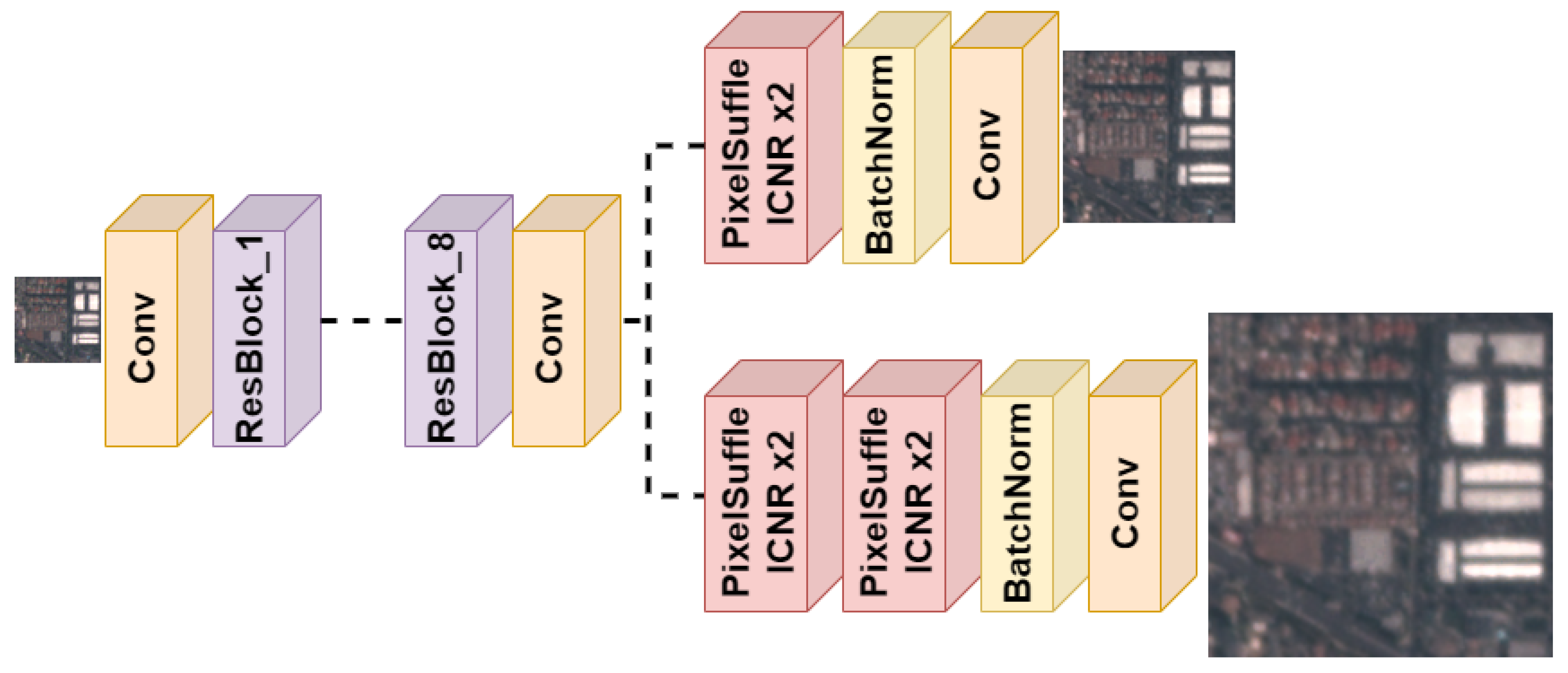
There are two main parameters used to define EDSR architecture—the number of ResBlocks and the number of filters in each ResBlock. Increasing the number of ResBlocks and filters may lead to an increase in terms of performance, but the computational resources required for larger networks may also be very demanding. Moreover, when increasing the size of the network up to 32 ResBlocks and 256 filters, the authors found problems to stabilize the training. This issue was handled by introducing a residual scaling factor (default value of 0.1) after the last convolutional layer of the ResBlock. In our case, our preliminary results showed that using the scaling factor was also beneficial for the smallest EDSR and therefore, it will be applied to all cases. In the experiments, EDSR with 8 ResBlocks and 64 filters will be mainly considered, but the benefit of using 32 blocks with 256 filters will also be tested.

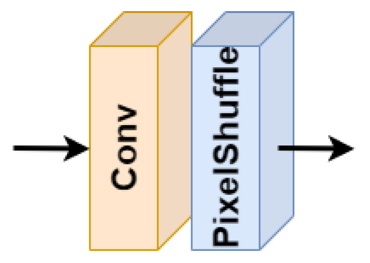
After the ResBlocks, EDSR use Pixel Shuffle upsampling to increase the resolution at the end of the network, which avoids the usage of bicubic interpolation prior to the network and its disadvantages. Pixel Shuffle layer consists of two main computations (Figure 2): (1) a convolution layer to increase the number of filters to the size required by the next step; (2) a shuffle operation that rearranges the activations in the feature maps to obtain shallower but larger feature maps, with the same number of activations [31]. Pixel Shuffle layer is applied once for 2× super-resolution and twice for 4× super-resolution. This approach allows one to perform progressive resizing to improve convergence, which consists of using a pre-trained model for 2× super-resolution to learn the 4× model, since the network only requires to introduce an additional Pixel Shuffle layer. This strategy will be tested in the experiments. A scheme summarizing the EDSR model used in this work is presented in Figure 3. Note that the only difference between EDSR8 and EDSR32 is just the number of ResBlocks and the number of filters in each ResBlock.

Regarding the loss function, as we have already mentioned, the authors proposed to substitute the commonly used L2 norm by the L1 norm, since they found that convergence was faster. Moreover, they also proposed the usage of a self-ensemble in testing phase, also known as test-time augmentation (TTA). For carrying out TTA, 8 different versions of the input image are first obtained (the original one plus flips and 90° rotations). Then, the network is used to compute the predictions for the 8 images. Finally, their mean image (after undoing transformations) is taken as output. In the original work, this model was named as EDSR+. In our case, we will also carry out the inference in this way, which is expected to give more robust results, although its benefits will also be evaluated in the experiments.

The rest of the modifications that we have introduced with respect to either the network or the training procedure are detailed in Section 3.3.

3. S2PS: Learning to Super-Resolve Sentinel-2 Using Planetscope

In this section, our proposal for super-resolving S2 RGBN 10 m bands to either 5 m or 2.5 m is explained. First, the motivation for the usage of PS as a reference satellite is presented in Section 3.1. How to create the training set for learning the model is then explained in Section 3.2. The modifications proposed for the EDSR network and its training procedure are presented in Section 3.3.

3.1. Proposal

The main problem when one aims to learn a CNN to super-resolve S2 images to resolutions greater than 10 m is that there are no ground truth images available at greater resolutions. To overcome this issue, our idea is to find a satellite with a sensor that is as much similar as possible to the S2 sensor (in terms of spectral bands), while providing images at greater spatial resolution. The sensor in Dove satellites (https://directory.eoportal.org/web/eoportal/satellite-missions/d/dove) met our requirements. The matching between the spectral bands of S2 and PS can be observed in Figure 4. In this specific case, the spectral bands correspond to S2-A satellite and group IDs 0cxx and 0dxx of PS. In fact, PS is a constellation formed of more than 120 Dove satellites. These satellites are divided into different groups with small variations in their spectral bands. The other key issue for selecting PS is that it has been operating since 2016. Hence, the operation period is similar to that of S2, making possible to obtain images of the same date and location, which is something we will require.

In our case, we have worked with the Ortho Tile Analytic products of PS (https://assets.planet.com/docs/Planet_Combined_Imagery_Product_Specs_letter_screen.pdf). These products are provided at 3.125 m resolution. Hence, they are resampled to both 5 m and 2.5 m using cubic interpolation for easing the architecture and learning of the network. We must acknowledge that we are not truly super-resolving S2 to 2.5 m, but we will be close to it. Apart from the reasons already explained, the possibility of freely accessing PS images following Open California program (details are given afterwards) has been a key point to use PS.

As it may be expected, ortho products from S2 and PS have different processing levels and magnitudes. In S2 products, reflectance with a scale factor 10,000 is represented. The processing level can be selected, being the Level-1C (L1C—top of atmosphere, TOA, reflectance) and the Level-2A (L2A—bottom of atmosphere, BOA, reflectance) the most widely used ones. Otherwise, the raster in the Ortho Tile product from PS contained digital numbers, as in many other satellite images. The metadata of the product was used to convert these numbers to TOA reflectance. Hence, the straightforward way to super-resolve S2 would be to use L1C together with PS images. However, L2A of S2 is the most widely used for a wide variety of tasks, since it better represents ground’s reflectance. Therefore, we preferred to work on this processing level. To do so, PS images with BOA reflectance were required. To achieve this, 6SV atmospheric correction was used (https://grass.osgeo.org/grass76/manuals/i.atcorr.html) [34,35] (with DEM from SRTM and the atmospheric model obtained using the water and ozone vapor values from MODIS satellite). This way, BOA reflectance was obtained for every PS product, making it comparable to S2 L2A products. As we will explain afterwards, this is a key issue, as both images must be as similar as possible, being their resolution almost the only difference. This is required not only to make the network learn a better model, but also to learn something that truly super-resolves S2, maintaining its properties. This is why the experiments also includes a spectral validation section to understand whether the resulting images are being biased towards PS or, as desired, only the resolution of the input images has been increased.

The rest of the processing required to close the gap between S2 and PS images is detailed in the next section. Clearly, not every pair of S2 and PS images will be valid. Among other requirements, they must have been taken under the same acquisition conditions (same ingestion date, close in time and close zenith observation angles).

3.2. Datasets

PS images were downloaded using 14 days free trial from Planet (https://www.planet.com/) giving access to Open California. Hence, all the images in our dataset are located in California state (United States of America, USA). In the future, we expect to extend the current study using images from other regions of interest.

Although the access to the images from PS is limited, the metadata for every image is available. This helped us finding the right images for our case study, as we will detail hereafter. When creating a dataset for SISR, the difference between the input and target images should be minimal and restricted to the resolution. The most common approach for standard images is to use a very high-resolution image as target and downsample it to create the input for the network. This is the ideal case is not applicable to S2. To simulate this process, images from a reference satellite (PS) will be used. Apart from looking for the proper satellite matching S2 properties, we must try to find the most appropriate images for learning. That is, we must look for images that are almost identical except for the resolution. Afterwards, the process followed is explained.

The first step consists of downloading product pairs from S2 and PS that match. Matching means that we will only download product pairs from the same location, acquired at the same date and with the minimal time difference. Furthermore, several filters are used for the query:

• Acquisition date: between 01/01/2017 and 01/01/2020;
• Cloud cover <10% in PS and <0% in S2;
• Minimum usable data: 90% in PS, not required in S2;
• The PS product must completely fall inside the S2 product.

Notice that these filters will not be applied when deploying the network, since it will be able to super-resolve any S2 image in L2A. Applying these filters, 257 different areas were found. Among them, in this work, we have considered the pairs of images presented in

Table 1. Summary of the images used from S2 and PS to form our dataset.

Area	Date	S2 UTC (UTC-7)	PS UTC (UTC-7)	Angle (S2/PS)	Set	#Tiles 2×	#Tiles 4×
Anderson	2019/06/20	18:49:21 (11:49:21)	18:37:39 (11:37:39)	9.0°/5.0°	train	2142	2214
Folsom	2018/06/29	18:49:19 (11:49:19)	18:20:12 (11:20:12)	2.4°/0.4°	train	2278	2334
Pasadena	2017/09/26	18:44:09 (11:44:09)	17:54:54 (10:54:54)	2.9°/3.6°	train	1596	1607
Patterson	2018/10/07	18:52:49 (11:52:49)	18:22:33 (11:22:33)	4.9°/0.1°	train	2071	1966
Santa Rosa	2017/07/19	19:03:51 (12:03:51)	18:11:00 (11:11:00)	7.1°/1.9°	train	684	687
Stockton	2018/10/17	18:53:59 (11:53:59)	18:19:31 (11:19:31)	3.6°/1.8°	train	1948	2080
Vallejo	2017/09/27	18:51:31 (11:51:31)	18:14:00 (11:14:00)	4.3°/1.7°	train	835	869
Willits	2017/08/26	18:59:09 (11:59:09)	18:17:18 (11:17:18)	2.7°/0.9°	train	1895	1897
Ontario	2019/03/30	18:29:39 (11:29:39)	18:10:25 (11:10:25)	1.9°/0.0°	val	2146	2166
Visalia	2018/09/10	18:39:21 (11:39:21)	18:12:50 (11:12:50)	3.6${}^{°}$/0.2${}^{°}$	val	1913	2077
La Habra	2018/08/29	18:29:09 (11:29:09)	18:00:59 (11:00:59)	1.5${}^{°}$/0.1${}^{°}$	test	2329	2348
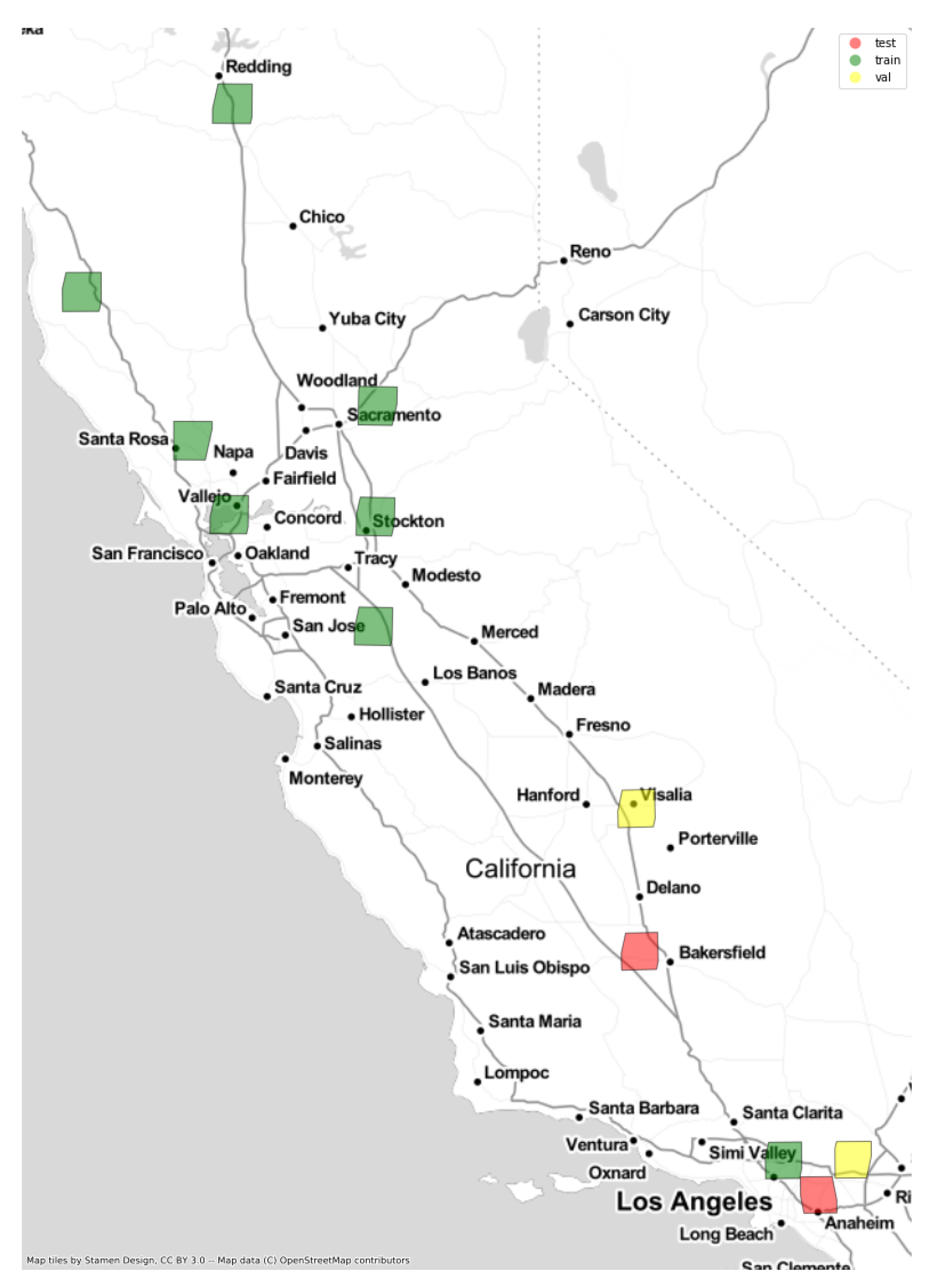
Shafter	2019/04/17	18:39:21 (11:39:21)	18:18:33 (11:18:33)	5.5${}^{°}$/2.1${}^{°}$	test	1529	1509

. Although we did not established any thresholds for the view angles, we checked them to ensure that they were as near as possible to the vertical (below 10°) and the difference with the corresponding S2 image was small enough (5.2° is the maximum difference in the dataset). For each image pair, the main area present in the image, the acquisition date and times (for S2 and PS), the view angle (for S2 and PS) and the set to which it is assigned together with the number of tiles obtained from this image (for 2× and 4× super-resolution, respectively) are presented. These images were selected to have a variety of scenarios, preventing non-urban areas from dominating the dataset (which would have occurred if all the areas were used). The locations in Table 1 are georreferenced in Figure 5.

Following the standard guidelines in Machine Learning [36], images were divided into three sets (partitions)—training, validation, and test. Each whole image is assigned to a single set to make the evaluation fairer. The idea is to use the training set to learn the parameters/weights of the network. The validation set serves for selecting hyper-parameters and doing early stopping (selecting the model with the lowest validation error rather than taking the last model obtained in training). Finally, the test set is used to check the generalization ability of the model, and in our case, to compare the different proposals. Zones (tiles) of the same image cannot be assigned to different sets because it could give one the impression that the model generalizes better than it really does, for example, if the model has memorized very similar zones (from the same image). The set to which each image has been assigned is shown in Table 1. Again, this split has been done in such a way that all three sets have a good representation of the different scenarios. The last two columns in the table indicate the number of tiles that are obtained from each image for 2× and 4× super-resolution, respectively. Images are divided into tiles to train the network, since the whole images would not fit into the GPU memory. Notice that different number of tiles are obtained from each image due to a validation process applied to make sure that tiles are useful. This process is explained later.

For S2, the S2 L2A products were directly downloaded only taking the RGBN bands, which are also present in PS images. For the PS Ortho Tile product, the BOA reflectance was computed as explained in Section 3.1. Co-registration accuracy of the satellites may slightly differ. This issue has been overcome automatically performing small shifts (maximum of 4 PS pixels, that is, 10 m) between image pairs if necessary (maximizing the PSNR between both images). Since the S2 products covered a larger area, they were cropped following the bounding box given by the corresponding PS products. Next, each image was divided into tiles (patches) of $48\times 48$ pixels for S2, and $96\times 96$ and $196\times 196$ pixels for PS 2× and 4× super-resolution, respectively. These tiles are the inputs and targets for our learning process. Nonetheless, although very similar reflectance values for each tile pair could be expected, they did not match exactly. There was some color mismatch that should be treated. The main source for this problem was the difference between the spectral bands. Our first attempt was to match them using the Spectral Bands Functions via SBAF [37], but we finally considered a simpler yet effective alternative known as Histogram Matching (HM) [38]. HM transforms an image in such a way that its histogram matches the histogram of a reference image. So, one can apply HM to PS images so that they better resemble the colors in S2 images. HM produces an even better result when applied to small tiles, which fits well our problem. In fact, this is the ideal situation to apply HM since tile pairs belong to the same location and have been acquired almost at the same time. HM for a pair of tiles is applied for each band as follows:

• To compute the cumulative histogram of each tile (S2 and PS).
• To linearly interpolate unique pixel values in the PS tile closely matching the quantiles of the unique pixel values in the S2 tile.
• To apply the learned pixel value transformation to the PS tile.

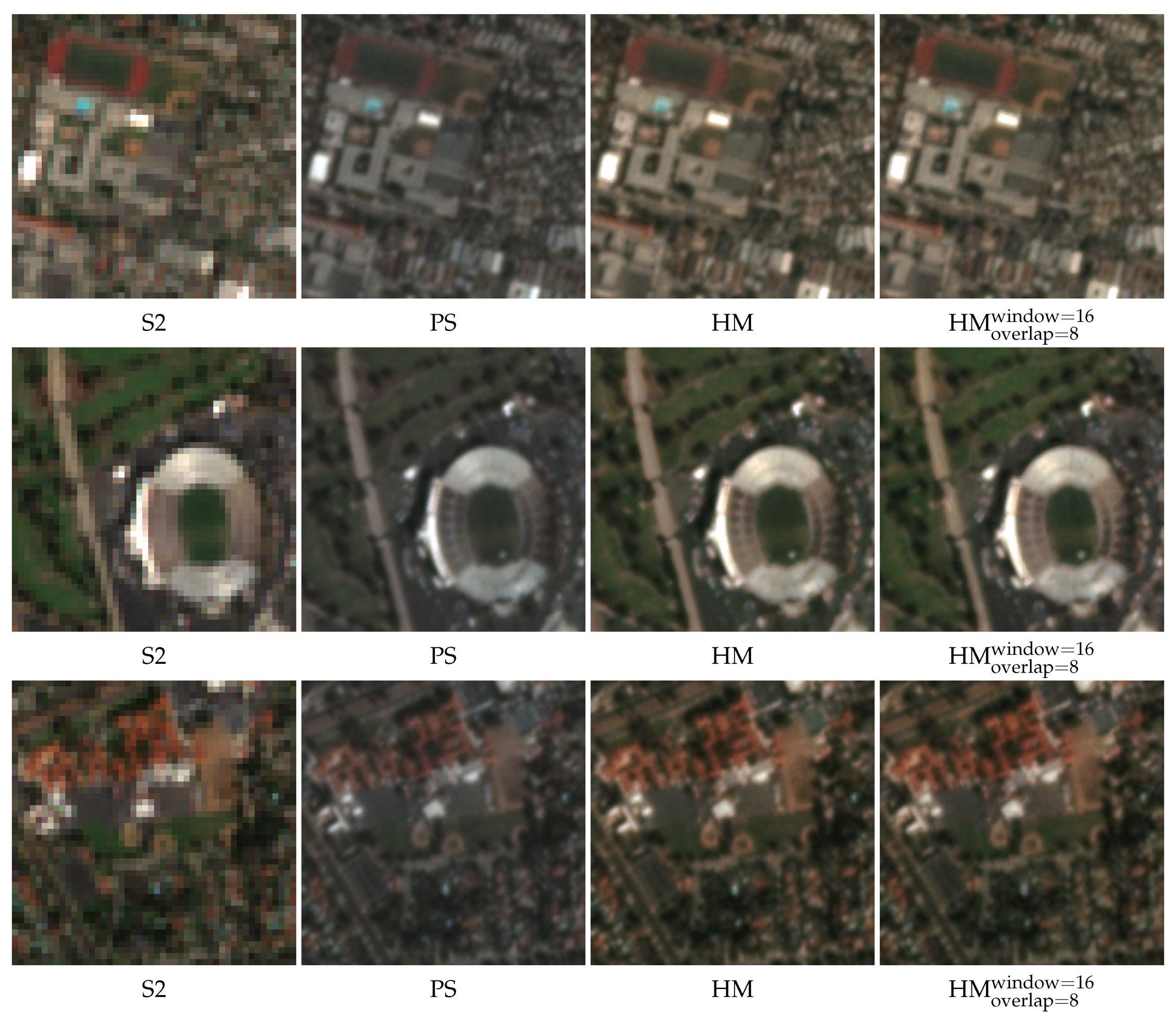
As a result, we will end up with a PS tile better matching the reflectance values of the S2 tile. However, although the tile size is relatively small, when applying HM to the whole tile a small color mismatch can still be appreciated. To solve this, our proposal is to apply HM in small windows of $16\times 16$ pixels with an overlapping among them (of 50%, that is, 8 pixels). Overlapping implies that for most of the pixels four values will be estimated, in these cases, the average value is then computed. Notice that the smaller the window size is, the better the reflectance matching is. However, there is a point where using a very small window size leads to a resolution loss, which should be avoided. Figure 6 shows the effect of applying HM to PS with S2 as a template. Both the case where HM is applied to the whole tile and the case where HM is applied by windows ($16\times 16$) with overlapping (8 pixels) are presented. Notice that 16 pixels refer to the window size in S2 tile (equivalent to 64 pixels in the PS patch of 4× and 32 pixels in that of 2×).

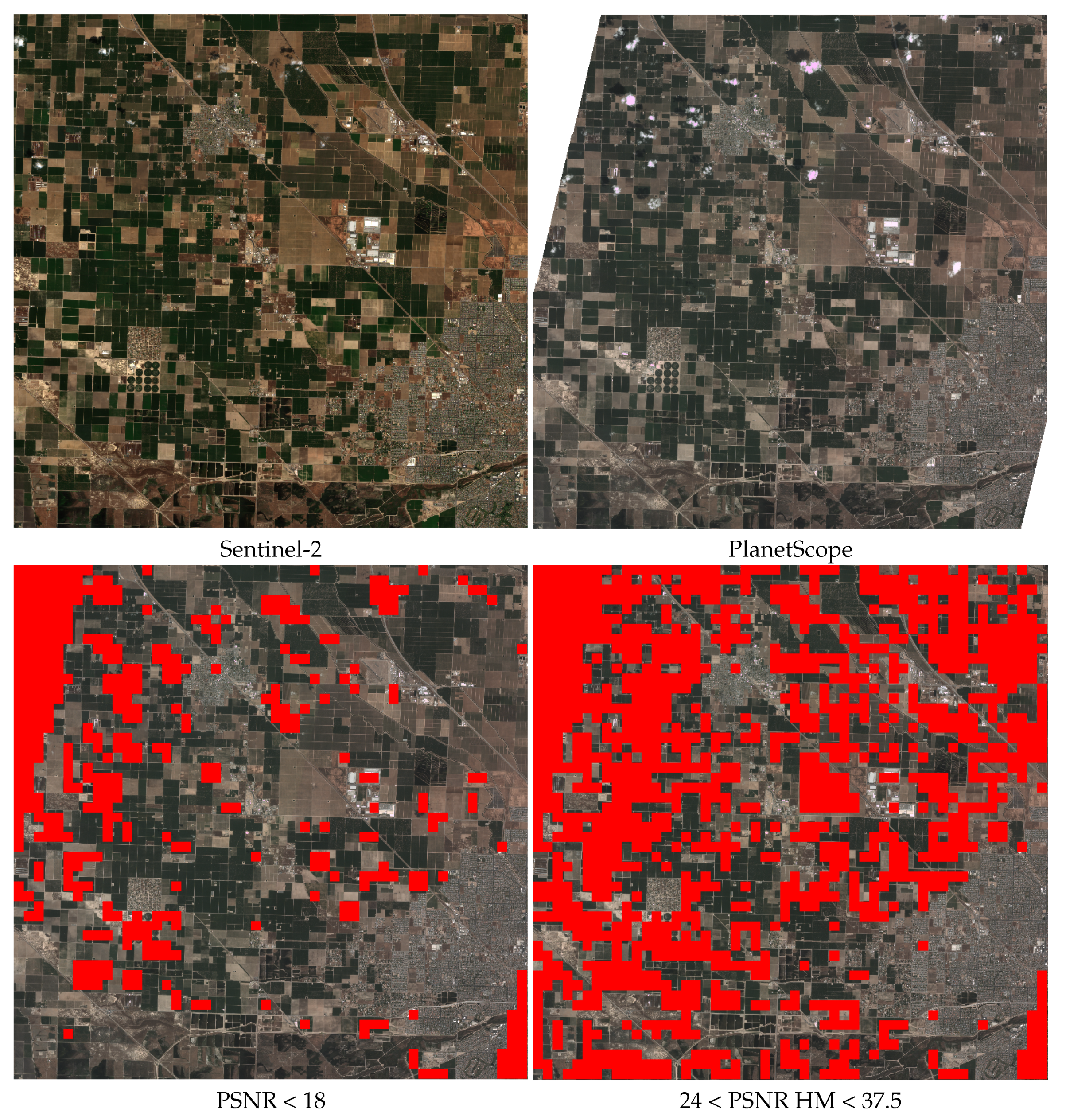
Although performing HM between tiles produces good quality tile pairs, there are still some undesirable patches that should be removed from the dataset (e.g., clouds or flat surfaces too similar to be useful such as sea, lakes, etc.). To filter these tiles, an automatic validation process is carried out based on the PSNR and SSIM metrics between S2 and PS tiles (these metrics are recalled in Section 4.4). The process is composed of three steps:

• To apply bicubic interpolation to the S2 tile to upsample it to the shape of the PS tile.
• Before applying HM—To compute the PSNR between the upsampled S2 tile and the PS tile and keep only those with PSNR higher than 18.
• After applying HM—To compute the PSNR between the upsampled S2 tile and the PS tile and keep only those with PSNR between 24 and 37.5.

The thresholds were established by visual inspection. SSIM was also considered for filtering, but the minimum quality required was always fulfilled by the patches passing the previous filters and hence, we decided to avoid this additional step. The two filtering steps can be explained as follow. The former is devoted to the elimination of patches where clouds or cloud shadows are present. In those cases, validating after HM can lead to high PSNRs, since the HM can completely change the appearance of the PS image making it very light or dark. The latter is devoted to remove other artifacts and patches that are too similar to be useful. This way, the quality of the dataset is ensured, avoiding those patches that do not provided any knowledge for the network. The result of applying this validation process to an image of the dataset (Shafter area) is presented in Figure 7.

The last step of the data preparation process is to normalize the reflectance values to $[0,1]$ interval for learning the network. This is done using the 12-bit range.

All the steps described to create the dataset can be summarized as follows (see also Figure 8):

• To download the data from PS (Ortho Tile Analytic product) and S2 (L2A product), only considering RGBN bands.
• To convert PS images to BOA reflectance values (using 6SV) and resample it to 5 m and 2.5 m (from 3.125 m).
• To match each PS image with the corresponding S2 image and crop the latter accordingly (S2 images are larger in size).
• To split the images into non-overlapping pairs of tiles. The tile sizes are $48\times 48$ for S2, $96\times 96$ and $192\times 192$ for PS (5 m and 2.5 m, respectively).
• For each tile pair, carry out HM to transform the PS tile, making it resemble what one could expect from a S2 image at greater resolution. HM is applied for each band using windows of $16\times 16$ pixels in S2 tile (with 8 pixels overlap). This process is carried out separately for the 2× and 4× datasets.
• To carry out the automatic validation of tiles using PSNR thresholds.
• To normalize the patches to $[0,1]$ using 12-bit range.

The number of tiles obtained for each area (image) are presented in Table 1.

Table 2. Number of tile pairs generated for training, validation and test for 2× and 4× super-resolution.

Set	#Images	#Patches 2×	Ratio 2×	#Patches 4×	Ratio 4× %
Train	8	13,449	63%	13,654	63%
Val	2	4059	19%	4243	19%
Test	2	3858	18%	3857	18%
Total	12	21,366	100%	21,754	100%

also presents the total number of tiles in each partition (training, validation and test). These numbers are close to the standard ones usually considered for learning and evaluating machine learning models. Most of the data are used for training (approximately 65% of the tiles) and fewer data are used for validation and test (approximately 20% for each set).

3.3. Network Training

Doing SISR with satellite images implies several changes compared to working with standard images. Usually, one must deal with more than the three standard RGB bands. Consequently, modifications in the network architecture are required, which makes usually difficult or not possible to use pretrained models. In our case, the input of the network requires handling an additional band. Moreover, the output of the network should also be composed of all four RGBN bands. That is, a RGBN image is given as input to the network and another RGBN image is expected as output (with higher spatial resolution). These modifications can be easily made in current deep learning frameworks, but they have several implications when using loss functions that do not only depend on the pixel-wise difference between the output and the target like the pixel loss (L1). This loss function can be directly extended to an arbitrary number of bands. However, in previous works [14], we showed that combining the pixel loss with two losses based on VGG16 [30] network (feature [30] and style [39] losses) provided good results, avoiding the blurry effect caused by the pixel loss. In this work, we aim to test their differences in terms of performance and try out some adaptations to better model the presence of the infrared band. Hereafter, the different losses that will be considered in the experimental study are briefly described.

• Pixel loss (L1): The pixel loss is the sum of absolute pixel-wise differences, also known as L1-norm or MAE.
• Feature loss [30]: Feature loss refers to the fact that the features of the super-resolved image and the target one should be as similar as possible. One way to obtain those features is to use the encoder part of a CNN and compare the activations of both images in different layers of the encoder. For the feature loss, VGG16 network is usually considered. Notice that this is commonly combined with the pixel loss.
• Style loss [39]: The style loss was initially proposed for style transfer problems but has been successfully applied to SISR in combination with the feature and the pixel losses. In this case, the objective is to make the correlations among the activations in different layers of a CNN (generally, VGG16) as similar as possible.
• Feature and style losses for infrared band: Feature and style losses strongly depend on a pretrained VGG16 network. This network is usually pretrained with Imagenet [23], which consists of standard RGB images. Hence, this network cannot be straightforwardly applied to images with RGBN bands. In Reference [14], we proposed to divide the loss into two parts: RGB and NIR losses, each part being composed of three components (pixel, feature and style losses). The RGB loss is computed as usual considering only RGB bands. For NIR loss, this band is converted into a RGB image by copying the same band into the three channels. This way, VGG16 network can be applied and the corresponding feature and style losses computed. Finally, both parts are combined scaling the losses so that all bands have the same importance (the parameters for doing so are specified in Section 4.3). Notice that VGG16 may not be well suited for NIR band, although it is only used for feature extraction. Hence, we will also test this loss function removing the feature and style losses from the NIR part to check which option provides the best result.
• Normalized Difference Vegetation Index (NDVI) loss: This is a new modification that we propose in this work as a way to improve the super-resolution of the NIR band. Since VGG16 is not pretrained with this channel one could expect the focal and style losses not to work properly with the NIR band. One way to indirectly improve the NIR band is to maintain its coherency with the red band. The NDVI is a well-known relation between NIR and red bands commonly used for analyzing vegetation in satellite images. Our idea is to enforce the network to learn that the NDVI of the output image and the target image should be as similar as possible. More specifically, and due to problems found with the optimization procedure when directly using the NDVI, we simplified it and use as loss the L1-norm of the differences between the NIR and red bands of the output and target images, respectively.

The different loss functions tested in the experimental study are summarized in

Table 3. Loss functions considered in the experiments and their identifiers.

Id.	Loss
$L_1$	Pixel-loss (L1-norm)
$L_1+L_{f{s}^{RGB}}$	Pixel-loss + Feature and Style losses for RGB bands
$L_1+L_{f{s}^{RGB+N}}$	Pixel-loss + Feature and Style losses for RGB and NIR bands
$L_1+L_{NDVI}$	Pixel-loss + NDVI loss
$L_1+L_{f{s}^{RGB}}+L_{NDVI}$	Pixel-loss + Feature and Style losses for RGB bands + NDVI loss
$L_1+L_{f{s}^{RGB+N}}+L_{NDVI}$	Pixel-loss + Feature and Style losses for RGB and NIR bands + NDVI loss

. Details about the weights given to each component of the loss function and the parameters for style and feature losses are in

Table 4. Common parameters for all experiments.

Parameter Name	Value
VGG16 layers (feature/style losses)	3, 4 and 5 max-pooling inputs
VGG16 layer weights feature/style	0.15, 0.8, 0.05/12.5, 3200, 112.5
RGB/NIR/NDVI Loss weights	0.75/0.25/0.0125
Optimizer	Adam
Weight decay	1 × 10−7
Learning strategy	Once Cycle Policy (pct_start=0.9)

.

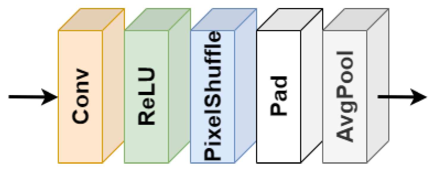
With respect to the architecture of EDSR, some updates apart from using other loss functions are introduced. These modifications focus on eliminating checkerboard patterns in the output image. The first one is to consider ICNR [17] initialization for Pixel Shuffle layers. The second one is to consider the proposal in Reference [18], which consists of blurring the output of the Pixel Shuffle layer with an average pooling operation (window size of $2\times 2$). The final scheme of the Pixel Shuffle layer used in this work is presented in Figure 9. Finally, as explained in Section 2.2, the authors of EDSR proposed to use a residual scaling factor (0.1) when training the largest versions of EDSR. After several preliminary experiments, we found that using this residual scaling factor also in EDSR8 led to better performance. Hence, we will consider it for all the experiments.

For training, the guidelines given by Leslie Smith in References [40,41] are followed, which usage has been extended thanks to fast.ai library [42]. There are two key points in this guidelines: the usage of the learning rate finder and the one-cycle policy for learning. Both are related and aimed at learning accurate models faster. The first one helps finding the proper learning rate, which makes a huge impact in what the network learns. The second one refers to make the learning rate vary in a specific manner so that the learning is more effective. Hereafter, we briefly recall how they work, but we refer the reader to the original papers, References [40,41] and the fast.ai book for more details [43]:

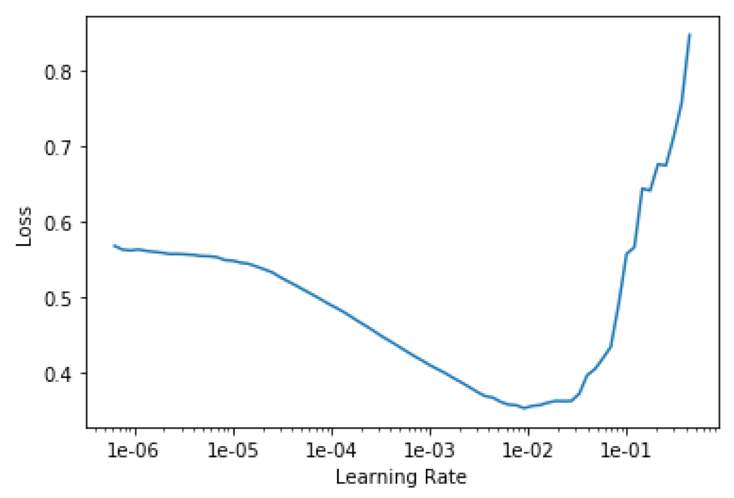
• Learning rate finder: The idea is to find a learning rate that is as high as possible so as to learn fast, but that it is not so high so as to diverge. To do so, before training, a very, very small learning rate is set and used to learn a mini-batch. Then, the learning rate is increased (e.g., doubled) and another mini-batch is processed, keeping track of the losses. This is done until the loss starts getting worse, which means that the learning rate is too high. Finally, one plots the loss in function of the learning rate (Figure 10) and selects a learning rate that is a bit lower than the one that achieves the minimum loss. The most common recommendation is to take an order of magnitude less than the minimum loss or the latest point where the loss clearly decreased.
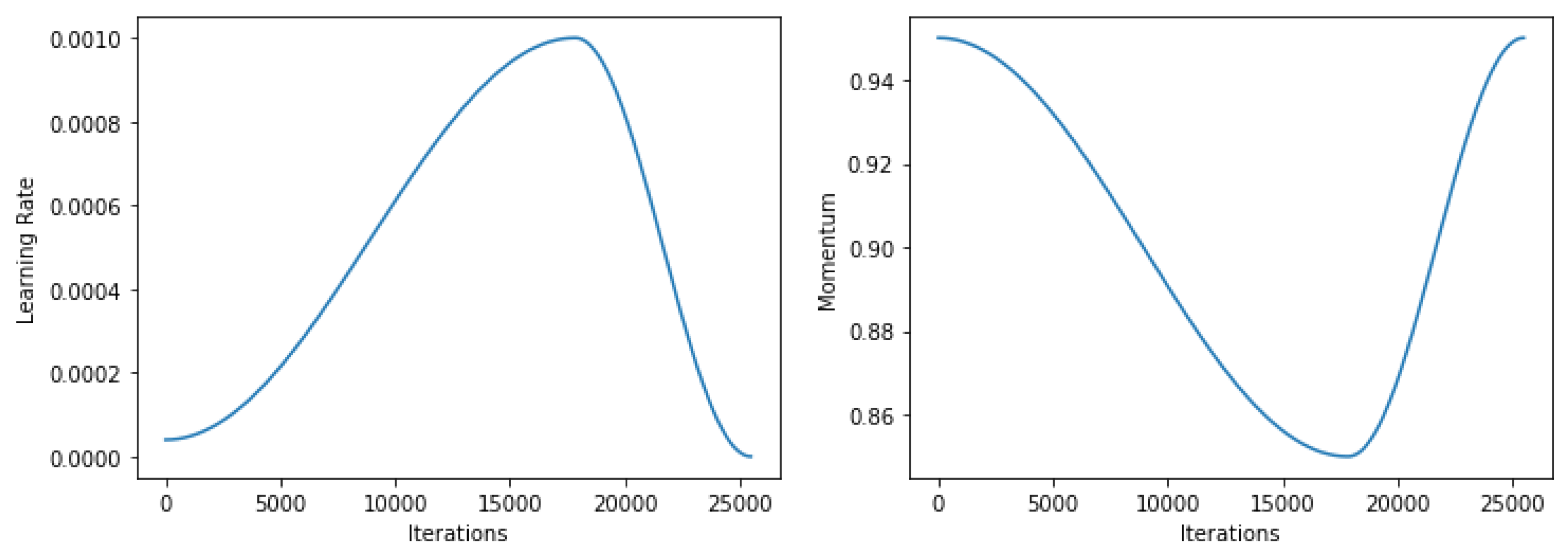
• One-cycle policy: In line with the learning rate finder, the one-cycle learning policy allows one to use higher learning rates to train faster and avoid falling in local minima. The idea is to start from a minimum learning rate and increase it during training to a maximum learning rate (that selected with the learning rate finder). Then, the learning rate starts decreasing to further optimize the solution in the current area. At the same time the learning rate goes up and down, the momentum will follow the inverse behavior. Figure 11 depicts how the learning rate and momentum values varies through learning. The moment when the learning rate starts decreasing is configurable, in this case set to 70% of the training.

According to the previous guidelines, we will use the largest batch size fitting into the GPU memory. The experiments have been run on a computing node with an Intel Xeon E5-2609 v4 @ 1.70 GHz processor with 64 GB of RAM memory and NVIDIA RTX 2080Ti GPUs with 11 GB of RAM.

In other respects, the progressive resizing idea presented by the authors of EDSR will also be tested. The idea is to reuse the model learned for 2× super-resolution when training the model for 4× super-resolution. In this manner, training the latter model can be done faster by simply adding another Pixel Shuffle layer to the 2× model. Since we will test both 2× and 4× super-resolutions, testing this idea for 4× super-resolution is straightforward and can give an idea of the usefulness of this strategy for S2 super-resolution. This process is carried out as follows:

• To train the 2× model (10 m S2 to 5 m PS) using learning rate finder and one-cycle policy.
• To introduce a new Pixel Shuffle layer to the 2× model to generate the 4× model (10 m S2 to 2.5 m PS).
• To train the new 4× model (only the new Pixel Shuffle layer and those after it, the rest are frozen) using learning rate finder and one-cycle policy.
• To train the whole 4× model further using learning rate finder and one-cycle policy with discriminative learning rates [44] (greater learning rates are assigned to the top of the network and lower ones to the earlier layers).

One key point here is the number of epochs run in each phase. Different combinations will be tested using more or fewer number of epochs for the 2× or the 4× model and comparing both the training times and performance of these models with respect to not using progressive resizing. More details about the specific configurations are given in the next section.

4. Experimental Framework

In this section, the experimental framework considered for the experiments in Section 5 is presented. First, the baseline models considered for comparison with our proposal are presented (Section 5.6). Then, in Section 4.2, the experiments carried out are summarized and justified. The parameters used for learning the networks are detailed in Section 4.3. Finally, in Section 4.4, the evaluation metrics that are used for the numerical evaluation in the experiments are recalled.

4.1. Models for Comparison

For the experimental comparison, we consider three different alternatives:

• Bicubic interpolation [28]: This is the well-known bicubic interpolation that considers $4\times 4$ pixel squares for interpolating new pixel values.
• EDSR trained on standard images (EDSR DIV2K): The first question with respect to CNN-based SISR for S2 is to consider whether it is really necessary to train a specific network on satellite images or networks trained on standard images could work to super-resolve S2. We will try to answer this question by comparing our proposal with a baseline model trained on standard RGB images and then applying it to super-resolve S2 images to 2.5 m. Obviously, this will be carried out only for RGB bands. To learn this model, DIV2K dataset [45] has been used, which consists of approximately 2K high-resolution images (800 for training and 100 for validation). These images are divided into patches, but no automatic validation process is required, since the low-resolution version (either $96\times 96$ or $48\times 48$) is obtained by bicubic downsampling the high-resolution patch ($192\times 192$, the same size as that of PS patches). The final dataset contains 55,510 patches for training and 7100 patches for validation. Testing is carried out on S2 to PS tasks.
• EDSR fully trained on S2 (EDSR S2S): This is the approach presented in References [5,6]. In this methodology, the idea is to learn to super-resolve S2 by learning a network using only S2 data. Since no ground truth data at 5 m or 2.5 m exist, one can downsample the S2 10 m bands to 20 m or 40 m, and use these as the input to the network and the 10 m bands as the target. This methodology is straightforward to implement, but as we will show in the experiments, it does not allow the network to learn the high-resolution details in 5 m and 2.5 m images. To implement this, the same image patches of S2 used for our network are considered, dowsampling them by bicubic interpolation as in the previous baseline model. Hence, this network will be trained with exactly the same patches as our proposal (but with different targets).

4.2. Summary of Experiments

In this section, we summarize the experiments that will be carried out in Section 5 and explain their objectives. There are several questions that we would like to answer:

• Which loss function works best for super-resolving S2?
• Does the NIR contribute to the super-resolution of RGB bands, and vice-versa?
• Is it worth doing progressive resizing?
• Could we take advantage of a larger version of EDSR?
• How big is the improvement obtained by TTA?
• Does the proposed model overcome baseline approaches?

The experiments are organized to answer these questions one by one. We will first test the different loss functions (Section 5.1). Then, we will compare the model learned for RGBN images with models learned separately for RGB and NIR bands (Section 5.2). We will continue testing the idea of progressive resizing (Section 5.3) and compare the EDSR8 model (the one used in most of the experiments due to the computational requirements of larger models) with EDSR32 (Section 5.4). Moreover, we will try to measure the gain obtained by applying TTA (Section 5.5) and end with the comparison with the baseline models (Section 5.6). This way, our aim is to get a complete overview of the different network and configuration variants that can be considered and show that the proposed approach is superior to existing models for S2 super-resolution.

All the experiments will be carried out under the same conditions. The parameters are shared by all of them except for the parameters depending on the model itself such as the learning rate (using learning rate finder) and the batch size. As we have already mentioned, all the experiments will focus on EDSR8 due to computational constraints, although we will also test the improvement that can be obtained with greater versions (EDSR32). For every experiment, we will learn two models, 2× and 4×. Obviously, the latter task is more difficult and our main objective.

4.3. Parameters

In this section, the parameters used in the experiments are detailed. The parameters that are shared by all experiments are presented in Table 4.

The specific parameters of each training are presented in

Table 5. Specific parameters of the training of the models in the experiments.

			$2\times$		$4\times$
Model	Loss Function	Epochs	Bs.	Lr.	Bs.	Lr.
EDSR8	$L_1$	50	64	1 × 10−3	32	1 × 10−3
EDSR8	$L_1+L_{f{s}^{RGB}}$	50	64	1 × 10−3	32	1 × 10−3
EDSR8	$L_1+L_{f{s}^{RGB+N}}$	50	64	1 × 10−3	32	1 × 10−3
EDSR8	$L_1+L_{NDVI}$	50	64	1 × 10−3	32	5 × 10−4
EDSR8	$L_1+L_{f{s}^{RGB}}+L_{NDVI}$	50	64	1 × 10−3	32	1 × 10−3
EDSR8	$L_1+L_{f{s}^{RGB+N}}+L_{NDVI}$	50	64	1 × 10−3	32	1 × 10−3
EDSR8 RGB	$L_1+L_{f{s}^{RGB+N}}$	50	128	1 × 10−3	32	1 × 10−3
EDSR8 NIR	$L_1+L_{f{s}^{RGB+N}}$	50	128	1 × 10−3	32	1 × 10−3
EDSR8 *	$L_1+L_{f{s}^{RGB}}+L_{NDVI}$	50	$64\times 2$	5 × 10−4	$32\times 2$	1 × 10−3
EDSR32 *	$L_1+L_{f{s}^{RGB}}+L_{NDVI}$	50	$56\times 2$	1 × 10−4	$16\times 2$	5 × 10−4
EDSR8 S2S	$L_1$	50	1280	1 × 10−3	1024	1 × 10−3
EDSR8 DIV2K	$L_1+L_{f{s}^{RGB}}$	50	48	1 × 10−3	32	1 × 10−3

Ep.: Epochs; Bs.: Batch size; Lr.: Learning rate; * multi-GPU training.

. In each row, the model, the loss function used for training and the number of epochs used for training are presented. Furthermore, the batch size and the learning rate for the 2× and 4× models are presented. The batch size can be increased when learning 2× with respect to 4×, since the output images are much smaller. Likewise, when only learning RGB or NIR bands, the batch size can also be increased. Regarding EDSR32, due to the size of the network, the batch size needs to be decreased. As a consequence, to obtain an accurate model, it becomes mandatory to run the experiments on multiple GPUs (accordingly, the batch size is doubled in our case using 2 GPUs).

The parameters used for testing progressive resizing are presented in

Table 6. Parameters considered in the progressive resizing experiments with EDSR8.

Model	Pre	Name	SR	Ep	Bs	Lr
1a	-	$S{2}^{10}\to P{S}^5$	2×	10	96	1 × 10−3
1b	1a	$S{2}^{10}\to P{S}^{2.5}$	4×	10	32	1 × 10−3
1c	1b	$S{2}^{10}\to P{S}^{2.5}$	4×	10	32	5 × 10−5, 1 × 10−4
2a	-	$S{2}^{10}\to P{S}^5$	2×	10	96	1 × 10−3
2b	2a	$S{2}^{10}\to P{S}^{2.5}$	4×	50	32	1 × 10−3
2c	2b	$S{2}^{10}\to P{S}^{2.5}$	4×	10	32	5 × 10−6, 1 × 10−5
3a	-	$S{2}^{10}\to P{S}^5$	2×	50	96	1 × 10−3
3b	3a	$S{2}^{10}\to P{S}^{2.5}$	4×	10	32	1 × 10−3
3c	3b	$S{2}^{10}\to P{S}^{2.5}$	4×	10	32	5 × 10−6, 1 × 10−5
4a	-	$S{2}^{10}\to P{S}^5$	2×	50	96	1 × 10−3
4b	4a	$S{2}^{10}\to P{S}^{2.5}$	4×	50	32	1 × 10−3
4c	4b	$S{2}^{10}\to P{S}^{2.5}$	4×	10	32	5 × 10−6, 1 × 10−5

Pre: Pretrained model; Ep: Epochs; Bs: Batch size; Lr: Learning rate.

. As we have explained in Section 3.3, 3 phases are trained in all cases. The difference lies in the number of epochs set in each phase (to pretrain the model for 2× and to train the new Pixel Shuffle layer).

4.4. Evaluation Metrics

The two most widely applied evaluation metrics for super-resolution are the peak signal-to-noise ratio (PSNR) and the structural similarity (SSIM) index [21]. Both measures will be used for the automatic validation (Section 3.2) and for the evaluation of the models.

The PSNR is based on the pixel-wise mean square error between the two images to be compared, in our case, the super-resolved S2 image and the PS with HM (target).

$$\mathrm{PSNR}(y,\widehat{y})=10·{\log }_{10}\left(\frac{v_{max}^2}{\mathrm{MSE}}\right),$$

(1)

where $v_{max}^2$ is the greatest possible difference between two pixel values, and

$$\mathrm{MSE}(y,\widehat{y})=\frac{1}{N·M·C}\sum _{i=1}^N\sum _{j=1}^M\sum _{k=1}^C{(y_{ijk}-{\widehat{y}}_{ijk})}^2,$$

(2)

where $N,M,C$ are the number of rows, columns and channels of the image, respectively.

Different from the PSNR, the SSIM is more focused on trying to model human perception, which can be more important than pixel-wise differences in certain contexts such as ours where the ground-truth is not a S2 image at 5 m or 2.5 m. SSIM computation is based on three terms that are computed in small windows along the image. These terms compare the luminance, contrast, and structure of the windows, which are then averaged to obtain the similarity between image pairs.

5. Experiments and Results

This section is divided into six parts, according to the experiment summary presented in Section 4.2. First, the best loss function is studied (Section 5.1) and the RGBN network is compared with independent RGB and NIR networks (Section 5.2). Then, progressive resizing idea (Section 5.3) and increasing the size of the network (Section 5.4) are tested. The usefulness of TTA is evaluated in Section 5.5. The proposed model is compared with baseline models in Section 5.6. Additionally, a spectral validation of the super-resolution is carried out in Section 5.7.

5.1. Loss Functions

In this first experiment the usage of the different loss functions is tested. Mainly, we want to compare the usage of pixel loss along with perceptual and style losses. Notice, however, that pre-trained VGG16 network may not suit well the NIR band. This is the reason why we proposed the usage of NDVI loss, which could help improving NIR band super-resolution.

Table 7. Peak signal to noise ratio (PSNR) and structural similarity (SSIM) metrics obtained by the different loss functions in the test set using test-time augmentation (TTA).

		$2\times$						$4\times$
		PSNR			SSIM			PSNR			SSIM
Model	Loss Function	RGBN	RGB	NIR	RGBN	RGB	NIR	RGBN	RGB	NIR	RGBN	RGB	NIR
EDSR8	$L_1$	33.42	34.23	31.88	0.9415	0.9466	0.9264	33.33	34.35	31.40	0.9142	0.9235	0.8862
EDSR8	$L_1+L_{f{s}^{RGB}}$	33.38	34.10	31.98	0.9409	0.9456	0.9270	33.21	34.18	31.37	0.9135	0.9225	0.8865
EDSR8	$L_1+L_{f{s}^{RGB+N}}$	33.19	34.14	31.39	0.9410	0.9459	0.9264	33.27	34.33	31.30	0.9124	0.9221	0.8836
EDSR8	$L_1+L_{NDVI}$	33.45	34.19	32.01	0.9418	0.9467	0.9273	33.28	34.27	31.40	0.9130	0.9221	0.8857
EDSR8	$L_1+L_{f{s}^{RGB}}+L_{NDVI}$	33.36	34.13	31.90	0.9409	0.9456	0.9268	33.34	34.30	31.48	0.9142	0.9231	0.8874
EDSR8	$L_1+L_{f{s}^{RGB+N}}+L_{NDVI}$	33.35	34.16	31.80	0.9410	0.9461	0.9258	33.28	34.32	31.31	0.9126	0.9224	0.8833

shows the results obtained for each loss functions when training EDSR8 network for both 2× and 4× super-resolution. For each model, the PSNR and SSIM metrics are evaluated on the test set. The values of the metrics for all four bands are provided in RGBN columns, whereas RGB and NIR columns provide the metrics computed for the corresponding channels separately. This allows one to get a global view of the results obtained. These results are obtained with TTA technique. The best value in each column is stressed in bold-face.

As it can be observed in Table 7, differences in terms of metrics among loss functions are rather small. In the simplest case (2×), losses based on pixel-wise differences ($L_1$ and $L_1+L_{NDVI}$) get a small advantage. However, when moving to the most complex case (4×), one can observe a shift in favor of using style and feature losses. The loss based on the combination of pixel loss, style and focal losses for RGB, and the NDVI loss ($L_1+L_{f{s}^{RGB}}+L_{NDVI}$) is the one achieving the best overall performance (RGBN) and also the best for NIR super-resolution. For RGB, it closely follows the pixel loss ($L_1$). 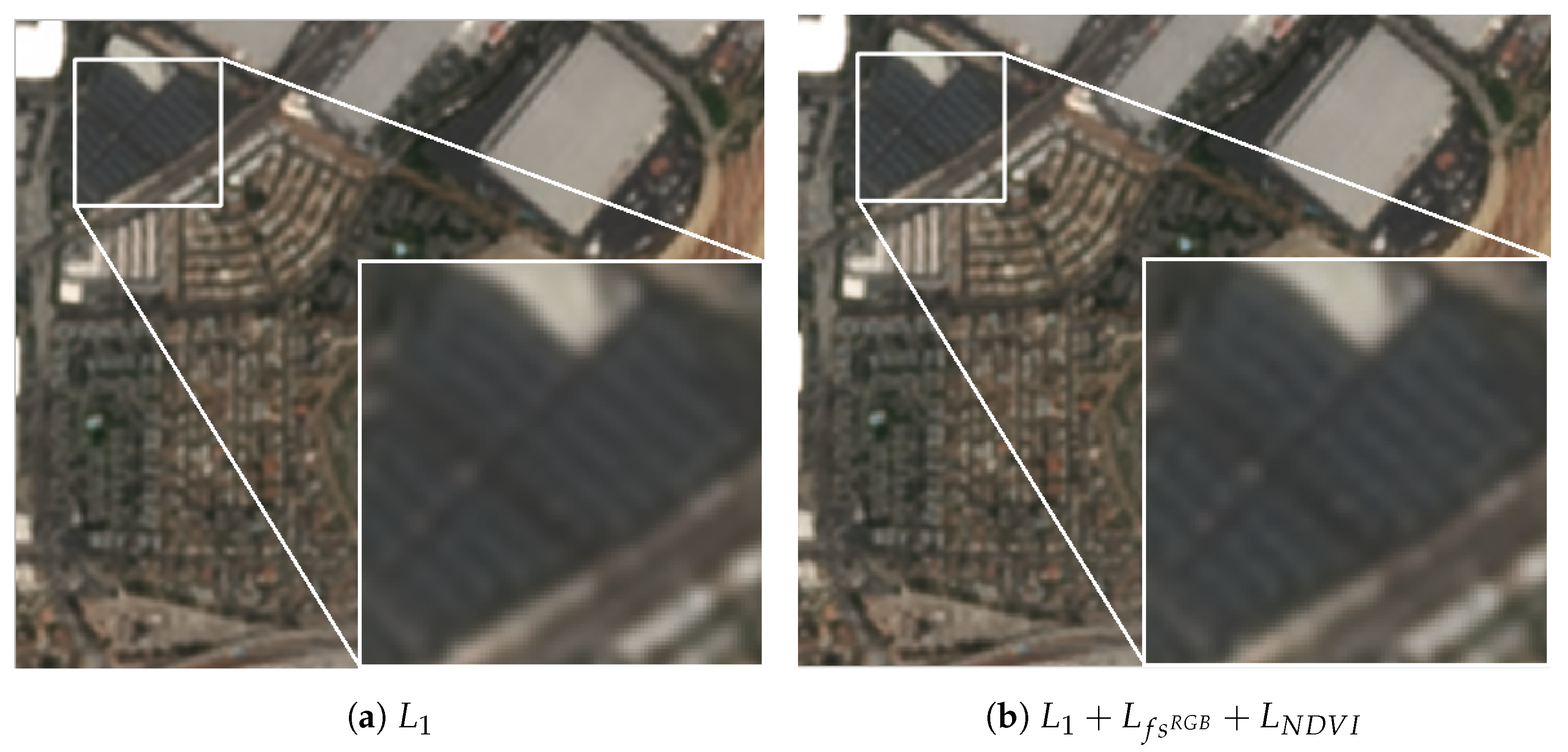Although these differences are not significant in terms of metrics, when closely looking at the images, one can observe the blurry effect produced by the pixel loss, which is avoided when introducing the feature and style losses. An example of this behavior is provided in Figure 12. Giving the best metrics for RGBN and NIR and also providing the best visual perception, the following experiments will use this loss function ($L_1+L_{f{s}^{RGB}}+L_{NDVI}$).

5.2. RGBN Vs. RGB and NIR

In the next experiment, our aim is to understand whether super-resolving all four RGBN bands at the same time truly helps when evaluating RGB and NIR separately. To do so, we have trained two additional EDSR8 models. One for super-resolving RGB bands (having 3 channels as input and output) and the other for NIR band (having 1 channel as input and output). In these cases, we cannot apply NDVI loss, since the information between RGB and NIR bands cannot be shared. Hence, we consider pixel loss along with feature and style losses for both cases (in the case of the NIR band, replicating the band to pass it through VGG16 network, since three bands are expected). The results of these experiments together with the best model found in the previous section are presented in

Table 8. PSNR and SSIM metrics obtained with different bands as input/output using TTA in the test set.

		$2\times$						$4\times$
		PSNR			SSIM			PSNR			SSIM
Model	Loss Function	RGBN	RGB	NIR	RGBN	RGB	NIR	RGBN	RGB	NIR	RGBN	RGB	NIR
EDSR8	$L_1+L_{f{s}^{RGB}}+L_{NDVI}$	33.36	34.13	31.90	0.9409	0.9456	0.9268	33.34	34.30	31.48	0.9142	0.9231	0.8874
EDSR8 RGB	$L_1+L_{f{s}^{RGB}}$	-	34.09	-	-	0.9451	-	-	34.09	-	-	0.9193	-
EDSR8 NIR	$L_1+L_{f{s}^N}$	-	-	31.93	-	-	0.9254	-	-	31.25	-	-	0.8795

(the best value in each column is stressed in bold-face).

These results clearly show that the model addressing the four bands at the same time takes advantage of them, allowing the super-resolution of RGB to complement the NIR one and vice-versa. The differences are larger in the case of 4×, where the individual models are always clearly worse than the one working with RGBN bands. Moreover, the approach using a single network is more efficient. Hence, we conclude that super-resolving all bands at the same time is beneficial.

5.3. Progressive Resizing

In the following experiment the usefulness of progressive resizing idea is tested. We run all the variants mentioned in Section 4.3 and learned different models. In this case, only the 4× super-resolution model can be evaluated, which is learned from the 2× model using progressive resizing technique. In this case, besides evaluation metrics, the training runtimes should also be evaluated.

Table 9. PSNR, SSIM and runtimes obtained by EDSR8 with progressive resizing technique using $L_1+L_{f{s}^{RGB}}+L_{NDVI}$ loss function and TTA in the test set.

		PSNR			SSIM			Runtime
Model	SR	RGBN	RGB	NIR	RGBN	RGB	NIR	(hh:mm:ss)
1a	2×	-	-	-	-	-	-	00:18:19
1b	4× (from 1a)	32.02	33.02	30.09	0.8835	0.8975	0.8415	00:55:01
1c	4× (from 1b)	32.86	33.73	31.16	0.9037	0.9121	0.8783	01:38:51
2a	2×	-	-	-	-	-	-	00:17:29
2b	4× (from 2a)	32.61	33.57	30.75	0.8972	0.9081	0.8645	03:26:56
2c	4× (from 2b)	32.73	33.52	31.14	0.9018	0.9105	0.8759	03:58:45
3a	2×	-	-	-	-	-	-	01:30:20
3b	4× (from 3a)	32.23	33.26	30.22	0.8926	0.9065	0.8508	02:06:09
3c	4× (from 3b)	32.77	33.69	30.95	0.9016	0.9116	0.8714	02:41:11
4a	2×	-	-	-	-	-	-	01:25:35
4b	4× (from 4a)	32.68	33.73	30.66	0.9016	0.9123	0.8694	04:14:25
4c	4× (from 4b)	33.02	33.95	31.22	0.9058	0.9145	0.8798	04:55:53
EDSR8	4×	33.34	34.30	31.48	0.9142	0.9231	0.8874	03:29:17

presents the results obtained using progressive resizing and compares them with the EDSR8 model directly trained for 4× super-resolution (the best value in each column is stressed in bold-face). The runtimes represent the total time needed to obtain a model. For example, for model 1b, we need to train 1a first, so the runtime for model 1b is that obtained for 1a plus the training time of 1b.

Attending to the results in Table 9, we can conclude that progressive resizing is not able to achieve the results obtained by the network directly learning the 4× super-resolution (last row). For every metric, this learning procedure is more effective. The most accurate model among progressive resizing approaches is 4c, but its runtime is even longer than the EDSR8 directly learning 4× super-resolution, since 50 epochs are run for the first two phases (4a and 4b). The case of 1c is more interesting, since it allows to quickly learn a super-resolution model (almost two times faster). Nonetheless, the performance of this model in terms of metrics is still far from the model not using progressive resizing. Hence, this experiment shows that progressive resizing can help in reducing runtimes, but it comes at the expenses of performance loss.

5.4. Deeper and Wider: EDSR32 with Multi-GPU

Following the findings of the authors of EDSR, the following experiment is aimed at testing whether increasing the size of the network (with filters and layers) pays off in terms of performance. To to so, EDSR32 network is compared with EDSR8. As we have explained in Section 4.3, EDSR32 required to use multi-GPU training to be able to set an appropriate batch size. For this reason, we have also re-run the experiments with EDSR8 using multi-GPU training to check that the possible benefit of EDSR32 is not simply due to this issue. The results obtained for EDSR8 with and without multi-GPU training and EDSR32 with multi-GPU training are presented in

Table 10. PSNR and SSIM metrics obtained with EDSR8 and EDSR32 using multiple GPUs and TTA in the test set.

		2×						4×
		PSNR			SSIM			PSNR			SSIM
Model	Loss Function	RGBN	RGB	NIR	RGBN	RGB	NIR	RGBN	RGB	NIR	RGBN	RGB	NIR
EDSR8	$L_1+L_{f{s}^{RGB}}+L_{NDVI}$	33.36	34.13	31.90	0.9409	0.9456	0.9268	33.34	34.30	31.48	0.9142	0.9231	0.8874
EDSR8 *	$L_1+L_{f{s}^{RGB}}+L_{NDVI}$	33.29	34.03	31.87	0.9400	0.9448	0.9259	33.12	34.03	31.33	0.9128	0.9218	0.8857
EDSR32 *	$L_1+L_{f{s}^{RGB}}+L_{NDVI}$	33.42	34.16	32.00	0.9411	0.9459	0.9268	33.70	34.79	31.66	0.9221	0.9323	0.8917

* multi-GPU training.

(the best value in each column is stressed in bold-face).

From these results, two main points can be stressed:

• EDSR8 is not capable of taking advantage of multi-GPU training, providing equivalent results.
• The larger EDSR32 network clearly allows one to make a difference in terms of performance with respect to EDSR8. This difference is notable in 4× super-resolution, increasing the PSNR (more than 0.6 points for RGBN and RGB and 0.3 for NIR) and SSIM values (almost one percent for RGBN and RGB and a half percent for NIR).

On this account, subsequent experiments will consider EDSR32 model.

5.5. Test-Time Augmentation

This experiment evaluates the usefulness of TTA technique. Recall that this technique uses the same network to super-resolve transformations (rotations and flips) of the same image. Then, the outputs are taken, and the transformation is undone so that the average image of the output for all transformations is taken as the final super-resolved image. Hence, it is cost free at training, but involves more computations at testing time. In this case, we have taken all the three networks in the previous experiment and compared the usage of TTA with not using it for each case. The results are shown in

Table 11. PSNR and SSIM metrics obtained with EDSR8 and EDSR32 in the test set using and not using TTA.

		2×						4×
		PSNR			SSIM			PSNR			SSIM
Model	TTA	RGBN	RGB	NIR	RGBN	RGB	NIR	RGBN	RGB	NIR	RGBN	RGB	NIR
EDSR8	no	33.91	34.76	31.90	0.9466	0.9514	0.9268	33.26	34.14	31.53	0.9127	0.9208	0.8883
EDSR8	yes	33.36	34.13	31.90	0.9409	0.9456	0.9268	33.34	34.30	31.48	0.9142	0.9231	0.8874
EDSR8 *	no	33.82	34.63	32.25	0.9455	0.9502	0.9311	33.10	33.95	31.42	0.9121	0.9205	0.8871
EDSR8 *	yes	33.29	34.03	31.87	0.9400	0.9448	0.9259	33.12	34.03	31.33	0.9128	0.9218	0.8857
EDSR32 *	no	33.97	34.79	32.38	0.9467	0.9514	0.9324	33.52	34.54	31.60	0.9234	0.9334	0.8933
EDSR32 *	yes	33.42	34.16	32.00	0.9411	0.9459	0.9268	33.70	34.79	31.66	0.9221	0.9323	0.8917

* multi-GPU training.

(the best value in each column is stressed in bold-face).

The results in Table 11 differ from what one could expect. TTA is not helping in terms of metrics in all cases. In fact, for 2× super-resolution, not using TTA provides better performance. When moving to 4× super-resolution, the PSNR for RGBN and RGB is always better with TTA, whereas for NIR, results vary although with small differences. With respect to SSIM, the benefit of using TTA depends on the network, for EDSR8 slightly better results are obtained when using it, whereas for EDSR32 not using TTA provides slightly better metrics. These results are against the intuition that using TTA should increase the robustness of the output, which should be reflected in better metrics. The key point here is that the super-resolution of S2 is being compared with a PS image (with the corresponding preprocessing). In this case, it seems that the networks have been able to learn some special characteristics of PS images such as the noisy textures present in the images. As a consequence, when doing TTA, these specific textures may get blurred due to the averaging of several images, which results in slightly lower metrics in some cases. Anyway, TTA as an ensemble mechanism usually provides more robust results, which is desired. Being differences in terms of metrics small and having enough computational capacity, we prefer to continue considering it, taking also into account that 4× super-resolution is our main objective (where differences are smaller).

5.6. Comparison with Existing Models

This section concludes the experiments by comparing the proposed EDSR model for the super-resolution of S2 images with the models described in Section 5.6. Recall that these models are the bicubic interpolation, an EDSR8 network learned only using S2 images and another EDSR8 network learned with standard RGB images. To carry out a fair comparison, we compare their results with our model using EDSR8, although we also provide the results of EDSR32. These results can be observed in

Table 12. PSNR and SSIM metrics obtained for the proposed and baseline models in the test set.

		2×						4×
		PSNR			SSIM			PSNR			SSIM
Model	Loss Function	RGBN	RGB	NIR	RGBN	RGB	NIR	RGBN	RGB	NIR	RGBN	RGB	NIR
Bicubic	-	32.80	33.33	31.76	0.9297	0.9320	0.9229	32.47	33.16	31.08	0.8925	0.8984	0.8747
EDSR8 S2S	$L_1$	32.93	33.64	31.56	0.9337	0.9382	0.9201	31.55	32.23	30.16	0.8712	0.8803	0.8440
EDSR8 DIV2K	$L_1+L_{f{s}^{RGB}}$	-	30.75	-	-	0.9151	-	-	32.00	-	-	0.8831	-
EDSR8	$L_1+L_{f{s}^{RGB}}+L_{NDVI}$	33.36	34.13	31.90	0.9409	0.9456	0.9268	33.34	34.30	31.48	0.9142	0.9231	0.8874
EDSR32 *	$L_1+L_{f{s}^{RGB}}+L_{NDVI}$	33.42	34.16	32.00	0.9411	0.9459	0.9268	33.70	34.79	31.66	0.9221	0.9323	0.8917

* multi-GPU training.

(the best value in each column is stressed in bold-face).

Looking at Table 12 one can observe the benefit of the proposed approach with respect to the baseline models. First, bicubic interpolation is the best among baselines except for the 2× super-resolution in terms of RGBN and RGB, where EDSR8 S2S achieves the best PSNR and SSIM values. Although S2S model seems to perform well for 2× super-resolution, when applied to 4× super-resolution the results are much worse than using bicubic interpolation. This is because the model is not capable of learning the details required for super-resolving to 2.5 m using images at 40 m and 10 m. The results of EDSR8 DIV2K are the worst ones, even for RGB bands (the only ones where it can be applied). This clearly shows the need for learning a specific network for satellite image super-resolution.

For every metric, the result obtained with our approach using EDSR8 outperforms all the baseline models. Notice, that these results are even better when using EDSR32. The low quality of S2S and DIV2K models is not due to the usage of EDSR8, but due to the problem being not adequately set out for super-resolving satellite images.

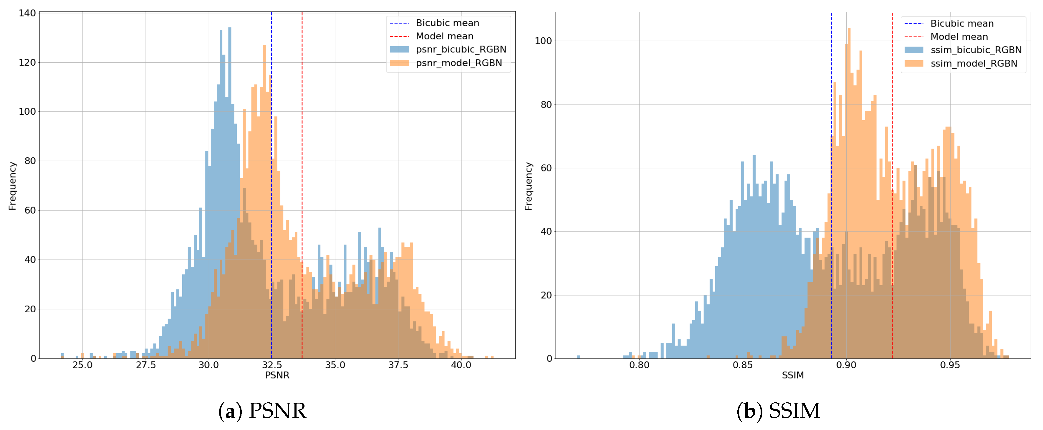
To better understand the differences between our best model and bicubic interpolation, Figure 13 represents the PSNR and SSIM values obtained for all tiles in the test set in the form of histograms. This way, one can observe how the proposed model tends to obtain more accurate representations moving the histograms to the right. Moreover, the greatest differences are found in the most difficult tiles (where bicubic gets lower PSNRs/SSIMs). This issue is even more accentuated in the case of SSIM, showing the great difference between both approaches.

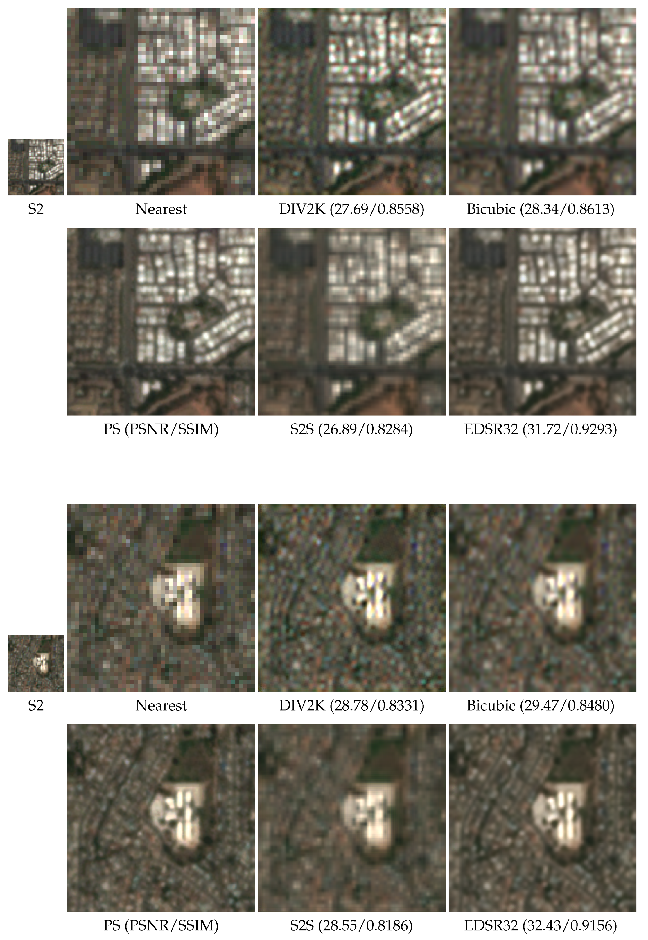
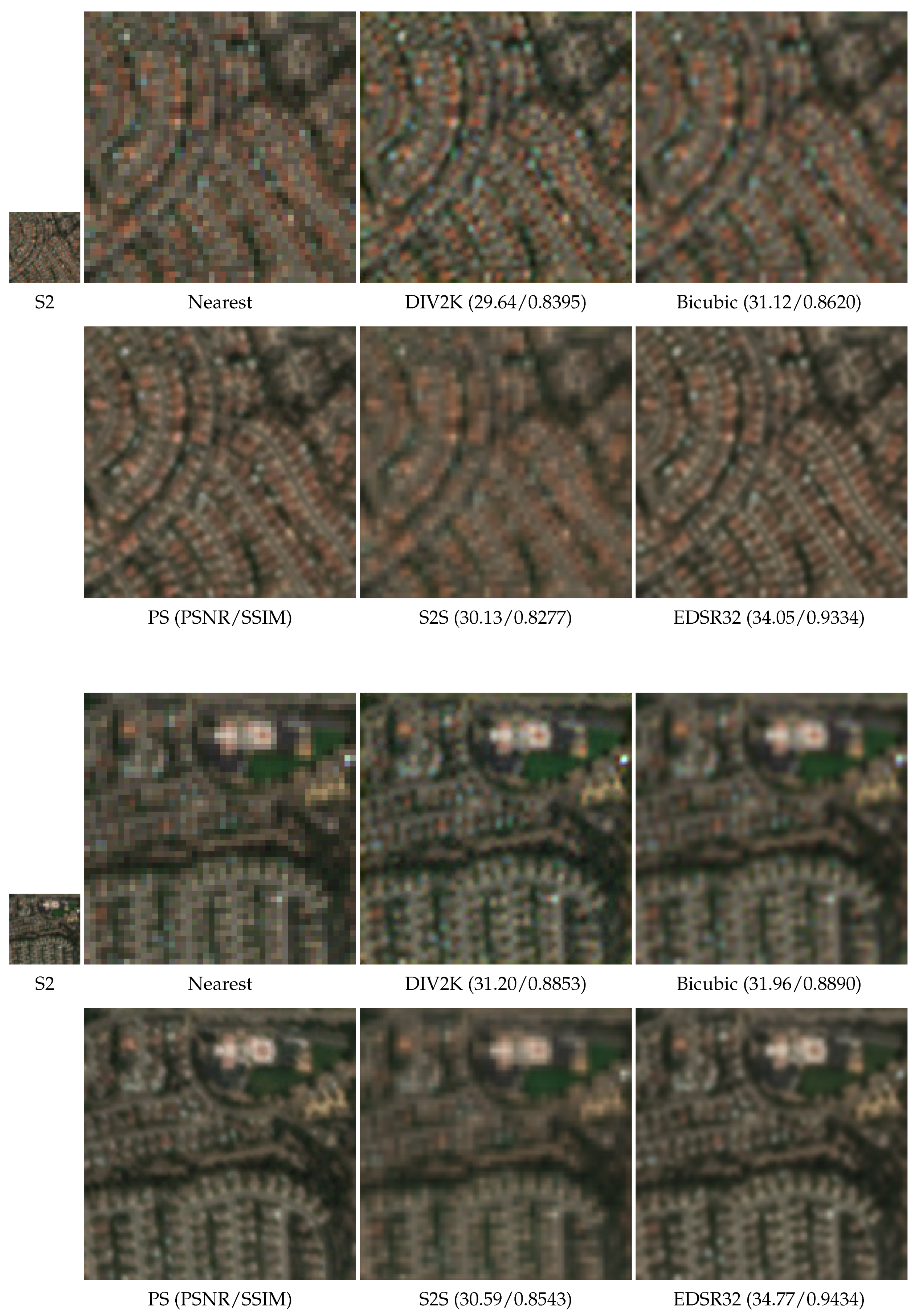
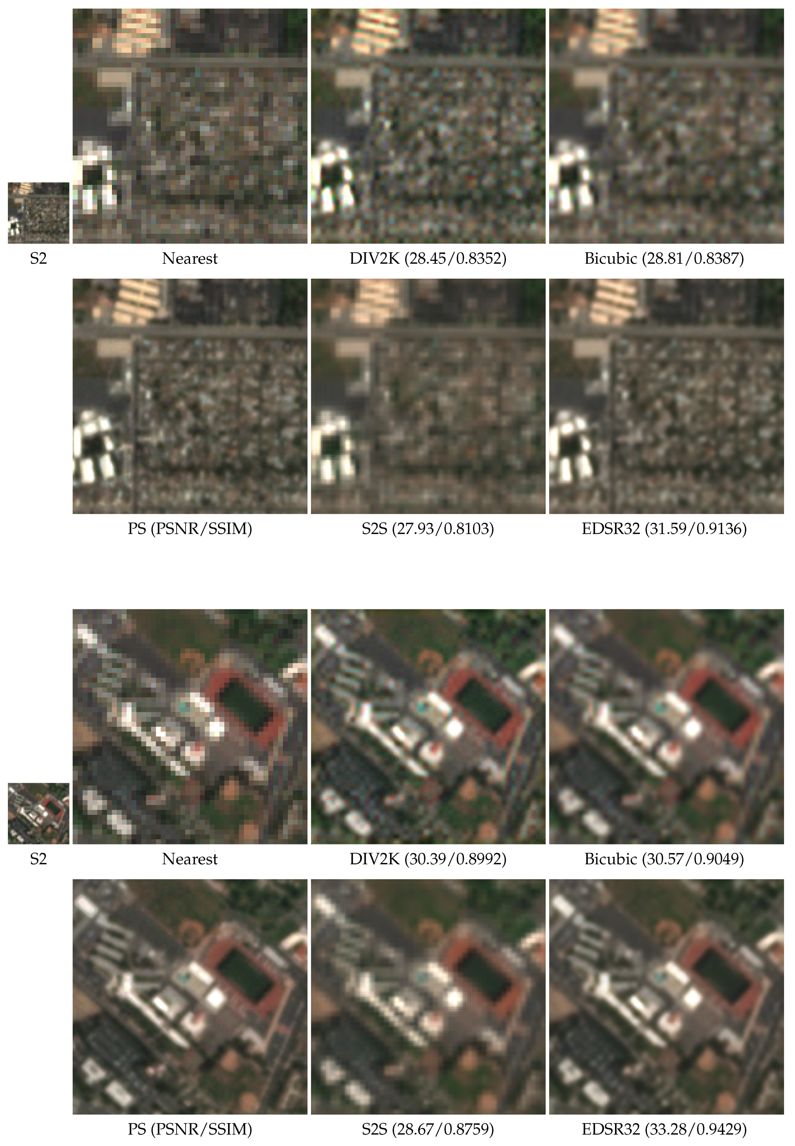
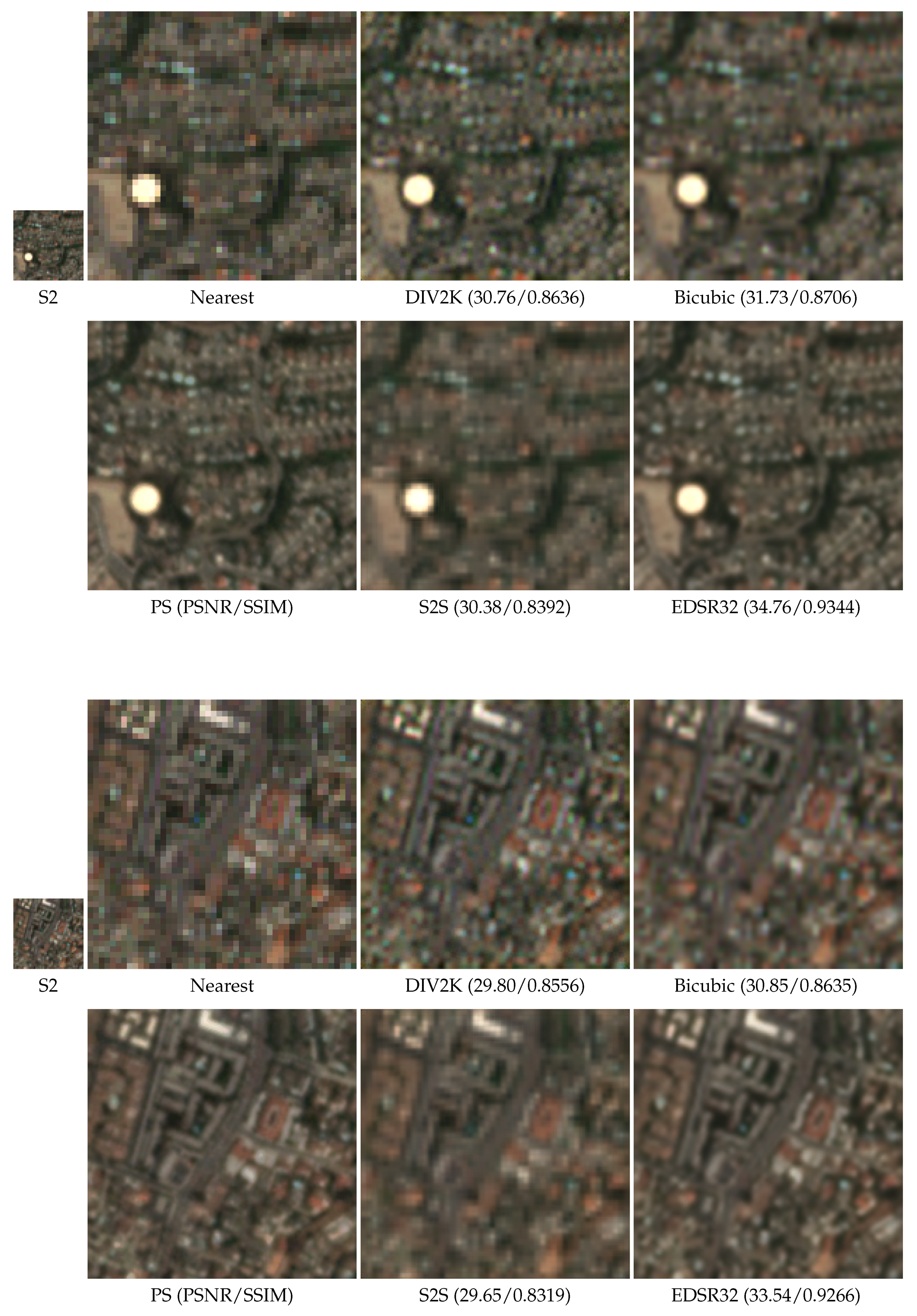
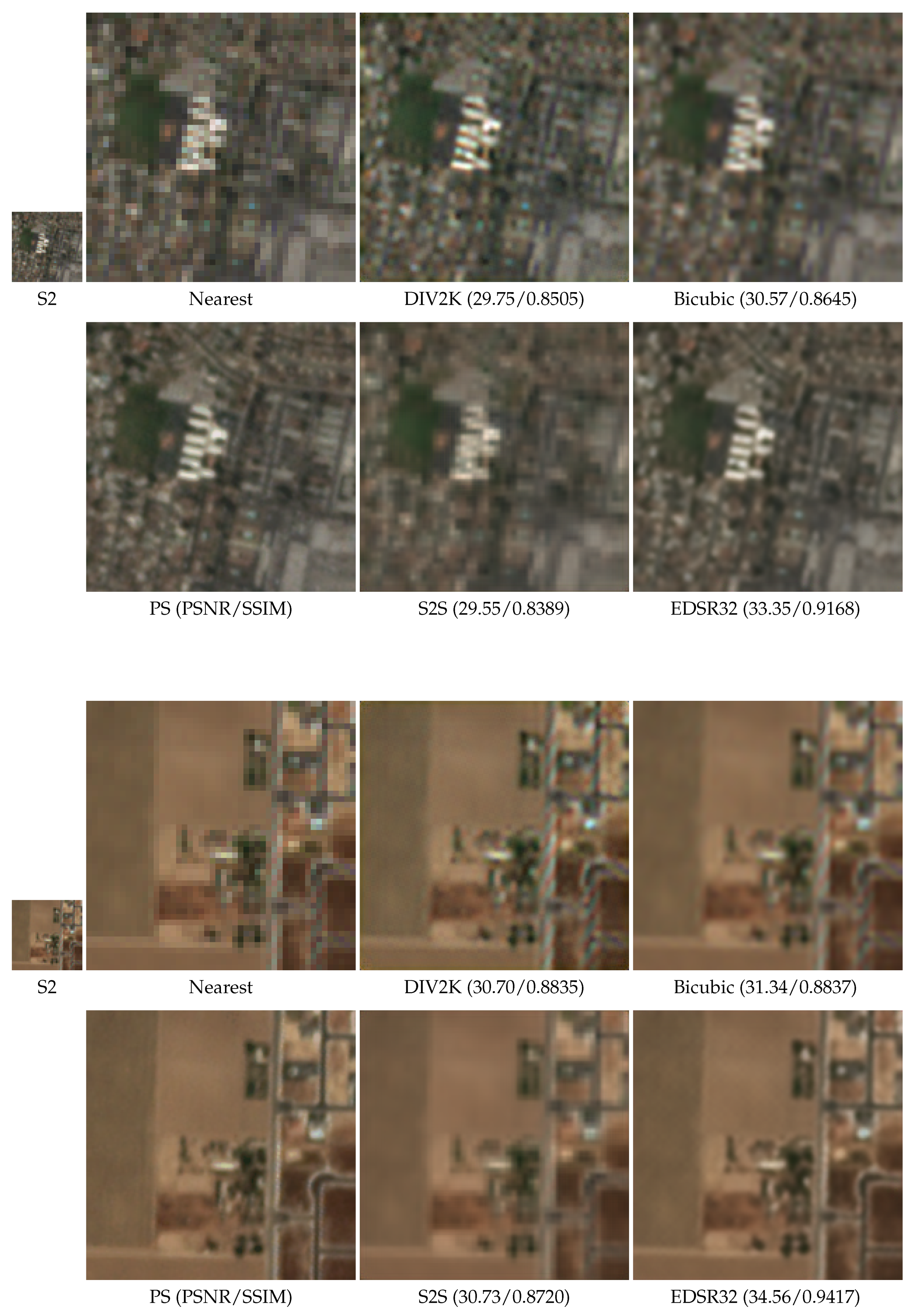
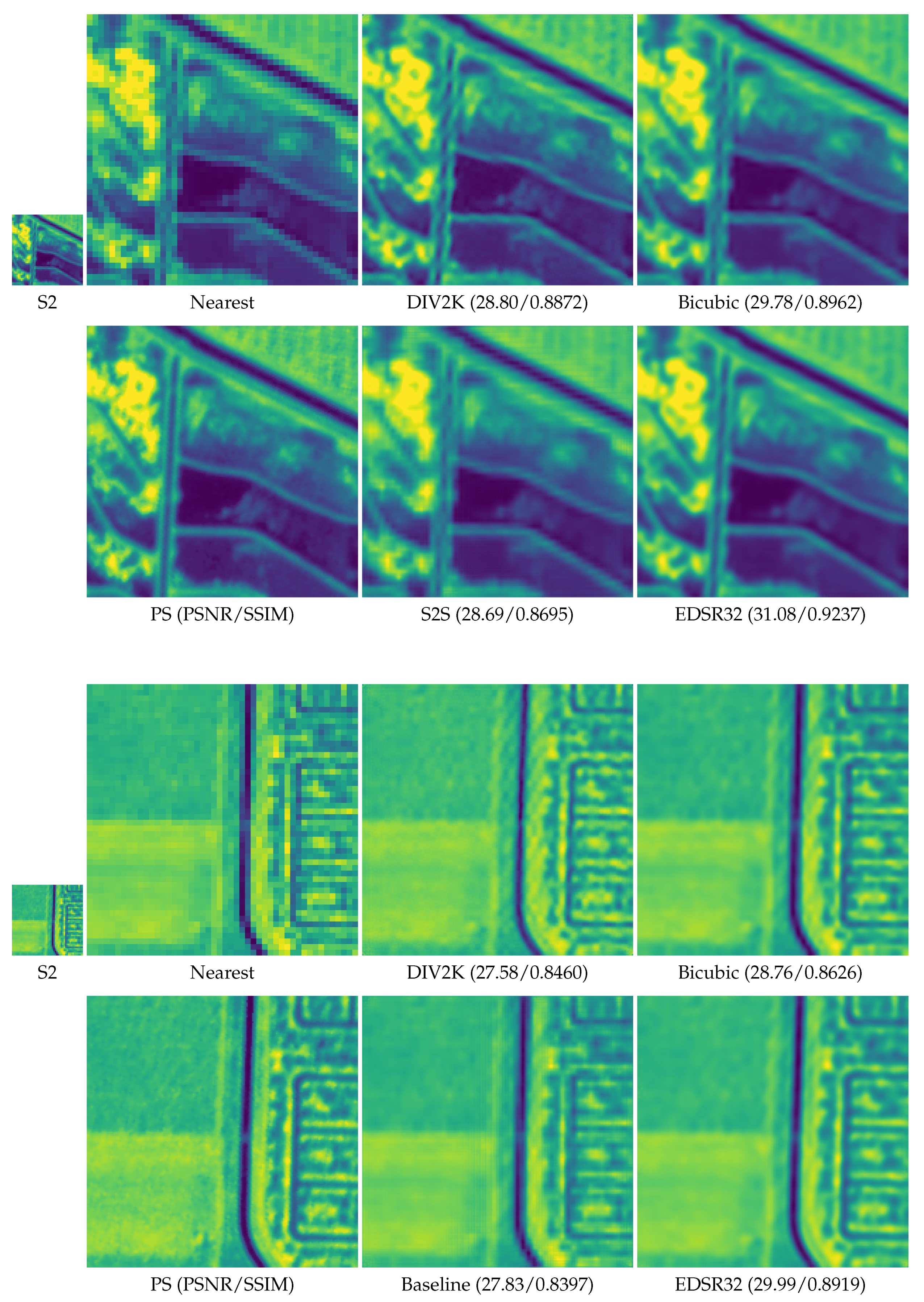
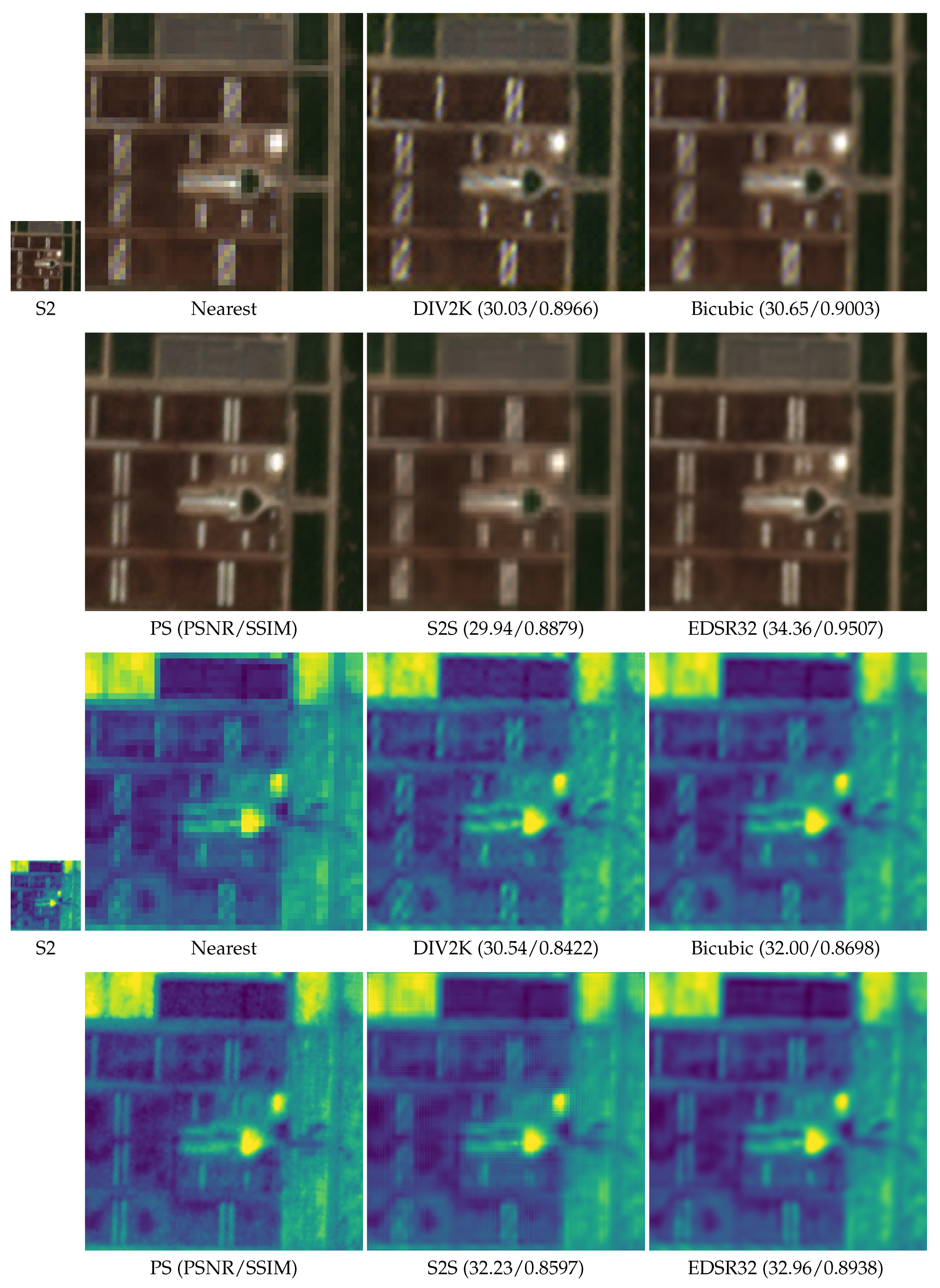
Overall, the proposed model works better in terms of metrics with respect to the baseline alternatives. This difference can also be visually observed. To do so, Figure 14 and Figure 15 compare the outputs of the different models with the desired output from PS (the last one corresponds to the NIR band). More examples are given in the Appendix A. We provide the visual result of nearest neighbor interpolation just to observe the information available for super-resolution at the same scale as the output images (the original S2 tile is represented in a smaller size although it covers the same area as the super-resolved images, but at a lower resolution). Visual results are provided for 4× super-resolution. Moreover, a complete map from the Iberian peninsula super-resolved using EDSR32 model is available at SEN4X webpage (https://tracasa.es/innovative-stories/senx4-at-the-cutting-edge-of-superresolution-technology/), which also shows the generalization capability of the model to other areas different from California.

Closely looking at these figures one draws the same conclusions as those looking at Table 12 with some additional information. DIV2K model shows the problems of applying standard models to satellite images. Although it is able to recover edges, some pixels get too saturated by blue and red colors, making the final image not represent the scene properly. Bicubic interpolation also does a great job, but the final results is blurry, being edges not so well defined. The case of S2S is even worse than bicubic in terms of blurriness. Details are not recovered and using this model seems useless compared to bicubic. Finally, EDSR32 model is the model best preserving colors and edges. Overall, it provides a nice visual result close to the target (PS). One should take into account that the only input data for this super-resolution is the S2 image. Bearing this in mind, the amount of information that it can recover is impressive.

5.7. Spectral Validation

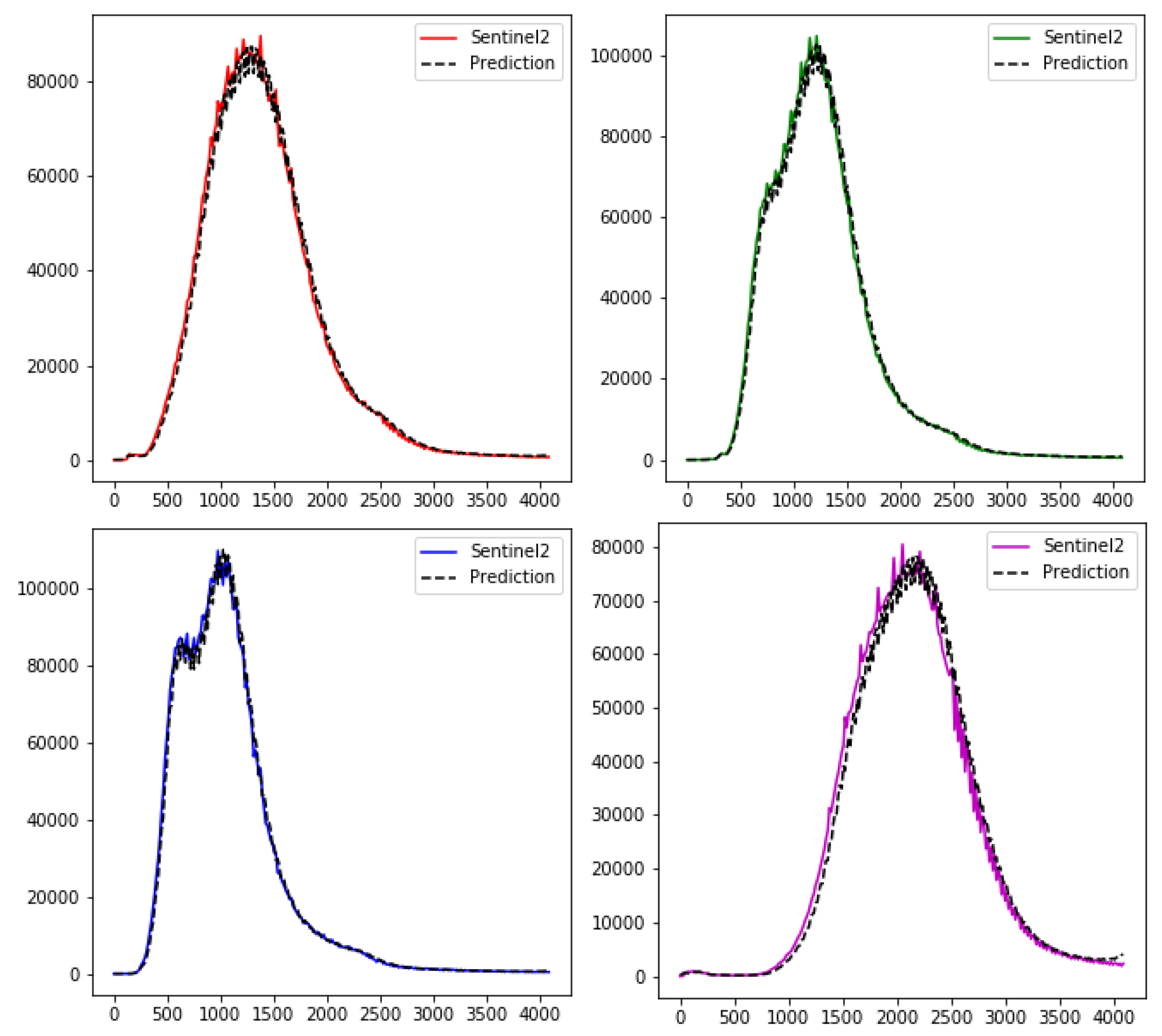
The goodness of the proposed methodology has been evaluated in the previous section. However, we have not carried out any validation of the reflectance values provided by the super-resolution. After super-resolving an image, we want to maintain the spectral radiometry with respect to the original S2, so that the same analyses can be carried out, but with greater details. To analyze whether these values are coherent with those provided by S2, we compare the histograms of a complete S2 image with the one obtained after its super-resolution with the proposed model (EDSR32). The histogram for each RGBN band is presented in Figure 16. For the sake of simplicity, the pixel counts (Y-axis) of the prediction are divided by 16, since 16 times more pixels are present in the super-resolved image.

As it can be observed, the histograms remain almost the same after super-resolution, which is a desired characteristic. Hence, the super-resolution is not altering the reflectance values. Anyway, differences must exist due to the additional details of higher resolution images.

6. Discussion

This section summarizes the findings of the experiments. The main conclusions drawn are the following ones:

• Loss function: Using NDVI loss has helped improving NIR super-resolution. Likewise, focal and style losses reduce the blurring effect of only using the pixel loss, although there are no big differences in terms of metrics.
• RGBN Bands: RGB and NIR bands complement each other when carrying out super-resolution. It is beneficial to learn to super-resolve all of them at the same time through the same network rather than learning a network for RGB and another for NIR, respectively.
• Progressive resizing: Despite being an interesting idea for accelerating learning, it has resulted in worse performance.
• Larger network: Increasing the capacity of the network from EDSR8 to EDSR32 was worth it, providing an increase in both PSNR and SSIM metrics.
• Test-time augmentation: TTA is known to increase the performance of CNNs. In our case, this has not been always the case. However, we acknowledge that this may be due to the fact that the input and output images comes from different satellites. However, we still prefer the higher robustness provided by TTA, since differences in terms of PSNR and SSIM are small.
• Comparison with previous models: The proposed methodology has clearly outperformed other models for S2 super-resolution. The well-known bicubic interpolation (a resampling method) has shown better performance than networks learned only with S2 images or using standard RGB images. Hence, the necessity for learning specific networks should be highlighted.
• Spectral validation: The proposed model has shown to maintain spectral radiometry with respect to the original S2 image after carrying out super-resolution, which is a mandatory characteristic.

7. Conclusions and Future Work

This work proposes a new methodology for super-resolving S2 RGB and NIR bands from 10 m to either 5 m or 2.5 m. To do so, a state-of-the-art convolutional neural network is used (EDSR) with several modifications for avoiding the presence of checkerboard patterns. To train the network, the main novelty of this work is the usage of a reference satellite with similar spectral characteristics (PS), which allows one to provide the network with higher spatial resolution images than those provided by S2. However, the usage of PS images matching those from S2 is not straightforward and there are several issues that must be taken into account: they should correspond to the same place and must be taken almost at the same time. Moreover, there will still be differences in the reflectance values. Our proposal considers histogram matching to solve this issue to make the radiometry of both images similar. With the dataset ready for learning, the learning rate finder and one-cycle policy are used to efficiently learn the network. Several experiments have been carried out to test the most appropriate loss function, whether using all RGBN bands at the same time helps each other, progressive resizing, TTA and the effect on the size of the network. Moreover, the proposed methodology has been compared with other alternatives for S2 super-resolution. Finally, some visual examples of their differences are provided, and a spectral validation has been performed. Overall, the proposed methodology has shown to provide better results than existing alternatives, showing the possibility of further increasing the resolution of S2 images using other satellite as a reference for training a CNN.

Nonetheless, there are still several research lines on this topic that should be addressed in the future. The dataset could be extended including more images for training, validation and testing. The location of these new images could cover different continents around the earth, providing the network with greater variety. Likewise, other reference satellites could be studied, which provide real 2.5 m resolution or even finer resolutions so that the real limit of the super-resolution is tested. Moreover, this methodology could also be tested to learn to super-resolve other satellites, finding the proper pairs. S2 has more bands apart from RGBN and hence, it will be interesting to consider their super-resolution further, either taking advantage of the current solution or finding other reference satellites with higher spatial resolution in those additional bands. Among the bands used in this work, NIR has shown to perform slightly worse than RGB. Methods for increasing the capacity of the network to better learn the super-resolution of this band should also be studied. With respect to the networks themselves, other models apart from EDSR could be tested such as those based on GANs, among others.