A Double Epipolar Resampling Approach to Reliable Conjugate Point Extraction for Accurate Kompsat-3/3A Stereo Data Processing

Abstract

Kompsat-3/3A provides along-track and across-track stereo data for accurate three-dimensional (3D) topographic mapping. Stereo data preprocessing involves conjugate point extraction and acquisition of ground control points (GCPs), rational polynomial coefficient (RPC) bias compensation, and epipolar image resampling. Applications where absolute positional accuracy is not a top priority do not require GCPs, but require precise conjugate points from stereo images for subsequent RPC bias compensation, i.e., relative orientation. Conjugate points are extracted between the original stereo data using image-matching methods by a proper outlier removal process. Inaccurate matching results and potential outliers produce geometric inconsistency in the stereo data. Hence, the reliability of conjugate point extraction must be improved. For this purpose, we proposed to apply the coarse epipolar resampling using raw RPCs before the conjugate point matching. We expect epipolar images with even inaccurate RPCs to show better stereo similarity than the original images, providing better conjugate point extraction. To this end, we carried out the quantitative analysis of the conjugate point extraction performance by comparing the proposed approach using the coarsely epipolar resampled images to the traditional approach using the original stereo images. We tested along-track Kompsat-3 stereo and across-track Kompsat-3A stereo data with four well-known image-matching methods: phase correlation (PC), mutual information (MI), speeded up robust features (SURF), and Harris detector combined with fast retina keypoint (FREAK) descriptor (i.e., Harris). These matching methods were applied to the original stereo images and coarsely resampled epipolar images, and the conjugate point extraction performance was investigated. Experimental results showed that the coarse epipolar image approach was very helpful for accurate conjugate point extraction, realizing highly accurate RPC refinement and sub-pixel y-parallax through fine epipolar image resampling, which was not achievable through the traditional approach. MI and PC provided the most stable results for both along-track and across-track test data with larger patch sizes of more than 400 pixels.

1. Introduction

Kompsat-3 and Kompsat-3A are Korean Earth observation/infrared satellites. They can acquire along-track and across-track stereo data for three-dimensional (3D) topographic mapping applications such as dense digital surface model (DSM) generation, 3D display, and topographic map drawing [1]. Stereo satellite data have high potential for many geospatial applications such as disaster monitoring [2,3], ground displacement measurement [4,5], and urban building modeling [6,7,8]. For most stereo applications, epipolar image resampling is necessary for efficient image processing and stereo display in a stereo plotter [9,10].

The requirements for good epipolar image resampling are near zero y-parallax and x-parallax linearly proportional to the ground height; hence, accurate sensor modeling such as that based on rational polynomial coefficients (RPCs) is necessary. Epipolar image-resampling algorithms [11,12,13] use sensor modeling information to establish accurate correspondence between the ground object space and the image space. However, the conventional positional accuracy of direct sensor modeling or raw RPCs range from a few pixels to hundreds of pixels depending on the satellite. Therefore, the bias compensation for the sensor modeling is performed using the conjugate points and ground control points (GCPs) that are obtained from in situ surveys or from existing geospatial data. In addition, the conjugate points and GCPs in the image space should not be skewed but well distributed over the entire image. Accurate sensor modeling achieves less than one-pixel-level of accuracy [14,15].

Sensor modeling using conjugate points and GCPs increases not only the absolute positional accuracy, but also the relative geometric consistency between the stereo data. However, some applications over inaccessible areas do not necessarily require GCPs when rapid 3D monitoring is the top priority and the absolute positional accuracy is the secondary concern. Even under these circumstances, the direct use of the raw RPCs from data providers may not satisfy the geometric consistency between the stereo images because the RPCs of each image contain errors due to the satellite ephemeris. Even in a single trajectory, a satellite changes its attitude to acquire overlapping data between stereo data acquisitions, resulting in geometric inconsistency between stereo data [16]. Therefore, reliable conjugate points must be extracted through image matchings and used for accurate sensor modeling to ensure high geometric consistency among the stereo data, which comprise relative orientation.

In terms of image matching, conjugate points are extracted using reliable image-matching methods that are generally classified into two types according to their similarity measures—area-based and feature-based methods [17]. The area-based methods use templates of a predefined size at each image and identify the peak of similarity between them for extracting the conjugate points. It works well in situations in which the geometric differences between images in terms of scale, rotation, and translation are not serious. In this situation, a search space of the sliding template can be geometrically constrained to identify the similarity peak associated with the location of the conjugate points. Mutual information (MI) [18], phase correlation (PC) [19], and least square matching [20] are representative area-based matching approaches. However, the area-based methods are likely to fail when the images show significant distortions or large geometric differences. The feature-based methods extract conjugate points based on representative points, e.g., dominant features, line intersections, and centroid pixels of close-boundary regions. The extracted representative points between images are matched with each other using descriptors or similarity measures and the spatial relationships. These methods can be applied even when images have significant distortions and geometric differences [21,22]. Scale invariant feature transform (SIFT) [23], speeded up robust features (SURF) [24], and binary robust invariant scalable keypoints (BRISK) [25] are representative feature-based matching approaches. However, the limitations of this method are that they find conjugate points from the entire image that usually has similar features and might result in a large number of mismatched pairs.

To reduce the number of falsely matched points extracted in these methods, the search space for finding the correspondences should be minimized. A limited search space for finding conjugate points enables successful extraction in both the area-based and feature-based methods. Since RPCs relating the ground object space and image space when the satellite image was acquired are available, a rough geometric relation between stereo images can be derived. Even raw RPCs, i.e., RPCs without bias compensation, improve the matching results by reducing the search space. Using trajectory information of the sensor is an example approach to reduce the search space for conjugate point extraction [26,27]. Coarse-To-Fine matching approach is also based on the concept to reduce the search space in the coarse matching step to extract the reliable conjugate points in a fine matching step [28,29]. However, geometrically overlapped images (or local templates of the images) with raw RPCs still include differences in the translation, scale, rotation, and shear because of the errors in the RPCs. These differences can cause a large number of false matches. Apart from reducing the search space, studies focusing on satellite imagery to improve the matching performance were also introduced. In [30], uniform robust SIFT was developed by extracting features focusing on the numbers and their distribution. Studies for extracting well-distributed conjugate points over the overlapping regions were conducted by splitting the region for carrying out the matching process [18,21].

Generally, the conjugate point extraction is carried out on the original image space. In the case that the similarity between the original stereo data is high, these approaches show decent performance with proper outlier removal. However, there are many cases when low similarity stereo sets show poor matching or failure. Therefore, it is important to increase the reliability of conjugate point extraction. Therefore, we propose a double epipolar image-resampling method for more reliable and robust conjugate point extraction and for generating precise epipolar images and accurate 3D processing. First, a coarse epipolar resampling is performed using raw RPCs, and this is followed by the conjugate point extraction and RPC bias compensation. Second, fine epipolar image resampling is performed with highly stereo-consistent RPCs for achieving good-quality 3D stereo data. The basic idea is that coarse epipolar images with even inaccurate RPCs should show better similarity than the original images for better conjugate point extraction. In addition, various image-matching methods, including the area-based methods—MI and PC—and feature-based methods—SURF and Harris corners together with fast retina keypoint (FREAK) description (hereafter, “Harris”), were tested for quantitative analysis of the conjugate points extraction performance between the proposed and traditional approaches.

The experiments were conducted for along-track Kompsat-3 stereo and across-track Kompsat-3A stereo data. We compared the performance of the traditional and proposed stereo data-processing approaches from the perspectives of conjugate point extraction, RPC bias compensation, and resulting y-parallax. For the traditional approach, we tested the matching methods for the original stereo data to investigate their conjugate point extraction performance. The conjugate points extracted by each matching method were used for relative RPC bias compensation [16]. The conjugate image points were used to generate quasi-GCPs by the space intersection using the RPCs, followed by the reprojection of the quasi-GCPs back to the stereo data to analyze the errors in the image space. The errors were minimized by applying bias compensation to the RPCs [31,32,33]. In contrast, for the proposed approach, we generated coarse epipolar images using the raw RPCs, followed by image matching with different methods and template sizes. The extracted conjugate points were transformed back into the original image space using the coarse epipolar image transformation parameters for relative orientation. Then, fine epipolar image resampling was performed with the bias-compensated RPCs. We analyzed the performances of conjugate point extraction, RPC bias compensation, and y-parallax for each case.

The paper is organized as follows: Section 2 introduces and elaborates on relative orientation. Section 3 provides the experimental results. The conclusions are presented in Section 4.

2. Methods

The flowchart of the study is presented in Figure 1. Figure 1a shows the traditional relative orientation-based epipolar image resampling. Given stereo satellite data with RPCs, image matchings were performed with outlier removal to extract conjugate points. We applied several matching methods, such as Harris, SURF, MI, and PC to investigate their conjugate point extraction performance. The extracted conjugate points were intersected for ground-point coordinate computation using the raw RPCs, i.e., for quasi-GCP generation. The quasi-GCPs were back projected to the image space to perform RPC bias compensation of the stereo data. Then, epipolar image resampling and y-parallax analysis were performed. Figure 1b shows the process when coarse epipolar image resampling is introduced before conjugate point extraction and RPC bias compensation, and this coarse resampling is followed by fine epipolar resampling; in other words, double epipolar resampling is performed. Image matching is performed for the coarse epipolar resampled images, and the performances were compared. The conjugate points extracted from the coarse epipolar images were transformed back to the original image space using the resampling transformation parameters. After RPC bias compensation, fine epipolar resampling was performed to ensure near zero y-parallax between the stereo data.

2.1. Epipolar Resampling

Stereo satellite data are resampled to satisfy the aforementioned epipolar condition (zero y-parallax and linear relationship between the x-parallax and ground height). Several epipolar image resampling algorithms [11,12,13] provide satisfactory results in terms of sub-pixel-level y-parallax. All these algorithms require accurate sensor modeling information such as RPCs to perform accurate projections between the ground object space and image space. In this study, we used the piecewise approach [11] that iteratively extracts epipolar curve points over entire images to establish epipolar image transformation. Figure 2 shows the epipolar curve pair extraction from the image-to-ground projection and the alignment of the epipolar curve to the same image line with an example satellite stereo data.

2.2. Conjugate Point Extraction

Extracting conjugate points with the help of RPCs that allow projection between the ground object space and image space can reduce the search area, thereby increasing the matching rate. The basic idea is that when even coarsely epipolar images are resampled with raw RPCs, i.e., without bias compensation, theoretically, it is possible to minimize dissimilarities (e.g., y-direction parallax, rotation amount, etc.) other than the x-direction parallax. In other words, we aim to demonstrate that the extraction of conjugate points from coarse epipolar images will be more advantageous than extraction from the original images. Therefore, two representative feature-based methods, SURF and Harris, and two representative area-based methods, MI and PC, were applied to the original and coarsely epipolar resampled stereo data, and the results were examined.

To detect well-distributed conjugate points over overlapping stereo images, local templates were constructed over the entire region with the same intervals in the x and y directions. When a template of one image (reference image) was determined, the location of the corresponding template of the other image (target image) was determined based on the coordinate information derived from the RPCs.

After extracting the conjugate points using each method, the outliers, that is, the falsely matched conjugate point pairs, were removed. To this end, the extracted conjugate points were used to estimate affine transformation coefficients, and the outliers with large root mean square errors (RMSEs) compared to other conjugate points were eliminated from the conjugate point set. The process of the outlier removal was repeated until all the remaining conjugate points satisfied the condition that the RMSE values were smaller than the predefined threshold. The target image was then warped to the coordinates of the reference image by using the estimated affine coefficients to calculate the correlation between the images to check the quality of the warping performance.

The detailed explanation of each matching method considering the local template concept is given in the following sub-sections.

2.2.1. Feature-Based Matching Using Local Templates

In this study, we adopted SURF and Harris approaches as examples of the feature-based matching methods. General feature-based matching methods that extract features and find correspondences from the entire image based on descriptor similarity result in a large number of mismatched pairs. To reduce such falsely matched points extracted in the feature-based methods, the search space for finding the correspondences should be minimized. To this end, the entire image was divided into regular templates, and the conjugate point extraction approach was applied to the corresponding templates [18,21]. More specifically, the template in the reference image was first constructed, and the center coordinate of the template was converted to the ground coordinates using the RPCs of the reference image. Then, the ground coordinate was converted to the coordinates of the target image using the RPCs of the target image. The corresponding local template of the target image was determined by selecting the image coordinate as the center of the template. According to the properties of the feature-based matching method, large numbers of conjugate points can be extracted for each corresponding template pair. To fairly compare the area-based and feature-based matching methods in terms of extracted numbers of the conjugate points, for each corresponding template pair, we extracted only the conjugate point that shows the highest similarity among the conjugate points.

The first feature-based matching method that we used is the well-known SURF algorithm proposed by Bay et al. [24]. The SURF algorithm uses the Hessian matrix to solve the problem of reduced repeatability and to increase the processing speed. Descriptors were generated to describe the characteristics of the extracted features. The SURF algorithm generates a 64-dimensional description vector that describes each feature by calculating the Haar-wavelet response value for the subdivided area. Finally, the ratio of the first to the second closest distances between the features described by the 64-dimensional description vector is calculated to extract the conjugate points.

In [34], authors compared combinations of well-known feature detectors and descriptors including Harris–FREAK, Hessian–SURF, maximally stable extremal regions (MSER)–SURF, and Fast–FREAK to identify the optimal detector and descriptor pair that best suits the matching procedure. Experiments conducted on 50 images revealed that the Harris–FREAK combination outperformed the other combinations. Therefore, as a second feature-based matching method, Harris–FREAK was adopted. In this method, a feature is identified by the Harris corner detector and creates a descriptor of each feature using the FREAK feature extractor [35].

The Harris detector [36] is invariant against geometric transformation and is resistant to change in illumination and noise. In this method, the corner point is detected based on the difference in pixel intensities measured using the auto correlation function. FREAK, which is inspired by the retina of the human visual system, is a keypoint descriptor [37]. A retinal sampling pattern is used for computing a cascade of binary strings by efficiently comparing image intensities. A binary descriptor is constructed by thresholding the difference between pairs of receptive fields with their corresponding Gaussian kernels. To combine the feature detector and descriptor, the FREAK descriptor is generated from the neighboring region of the point extracted from the Harris corner detector.

2.2.2. Area-Based Matching Using Feature-Centered Local Templates

PC and MI are the area-based matching methods used in this study. In such methods, generally, the center of the local template in the reference image is used as a feature, and its corresponding template in the target image is employed by using the geometric relationship between them. However, these methods do not work properly even in local regions since the center of the template rarely corresponds to a keypoint with a strong characteristic for descriptors, which provides the advantage of being extracted as a matching point. Therefore, we applied the area-based method in a local region where the center was extracted from a keypoint with a strong characteristic. Specifically, the center of each local template in the reference image was selected from the position of the strongest feature extracted based on the Hessian box filter used in the SURF method [24]. Then, the center of the template was converted to the ground location using the RPCs of the reference image, and the converted ground location was projected to the coordinate of the target image using the RPCs of the target image. The corresponding template of the target image was determined based on the position of its center for the matching process.

The PC approach was adopted to identify the similarity peak, which is associated with the position where the corresponding local templates show the optimal translation difference. The translation difference between template images in the x and y directions can be extracted by PC [19,38]. The method searches the difference in the frequency domain. Since we assume that the template images only have translation differences, the phase correlation values are approximately zero everywhere except at the shifted displacement. The location of this peak can be interpreted as the translation difference between the two corresponding local templates.

The MI method [18] matches two template images by measuring their statistical correlation. The MI value can be calculated using the sum of the entropies of the template images subtracted by their joint entropy. The larger the MI value between template images, the greater is the similarity between them.

2.3. Relative Orientation Based on Bias Compensation of RPCs with Outlier Removal

In photogrammetry, the relative orientation is basically the estimation of the position and orientation of one image relative to another from the correspondences of ray pairs without GCPs. For satellite sensors, the ray pairs are generated from extracted conjugate points using the rational function model (RFM) shown in Equation (1) [14]. The quasi-GCPs are computed by intersecting the light rays (Figure 3). Note that the light rays do not actually intersect if the RPCs, i.e., the coefficients of the RFM, are not sufficiently accurate, but they should be estimated by the least square adjustment. Because the quasi-GCPs are not on the light rays, the image coordinates of the quasi-GCPs also differ from those of the original image points when the ground coordinates of quasi-GCPs are back projected to the image space using Equation (2). These differences indicate the geometric inconsistency between the stereo data, and they must be minimized over the entire image using affine or polynomial relationships in the image space as shown in Equation (3). This minimization process is called RPCs bias compensation and well explained in [14]. In this study, we used the bias compensation to investigate how much accuracy the derived conjugate points can achieve from the proposed coarse epipolar image approach and the traditional conjugate point extraction method.

$$\begin{array}{l}l=RP{C}_l(\varphi ,\lambda ,h)=\frac{a^{T}u}{b^{T}u}{L}_S+L_0\\ s=RP{C}_s(\varphi ,\lambda ,h)=\frac{c^{T}u}{d^{T}u}{S}_S+S_0\end{array}$$

(1)

With

$$\begin{array}{l}u=[\begin{array}{ccccc}1& V& U& W& \begin{array}{ccc}VU& VW& \begin{array}{cc}UW& V^2\end{array}\end{array}\end{array}\hspace{0.17em}\hspace{0.17em}\hspace{0.17em}\hspace{0.17em}\begin{array}{ccccc}{U}^2& W^2& UVW& V^3& \begin{array}{ccc}V{U}^2& V{W}^2& V^{2}U\end{array}\end{array}\\ \hspace{0.17em}\hspace{0.17em}\hspace{0.17em}\hspace{0.17em}\hspace{0.17em}\hspace{0.17em}\hspace{0.17em}\hspace{0.17em}\hspace{0.17em}\begin{array}{ccccc}{U}^3& U{W}^2& V^{2}W& U^{2}W& W^3\end{array}{]}^T\end{array}$$

$$U=\frac{\varphi -{\varphi }_O}{{\varphi }_S},V=\frac{\lambda -{\lambda }_O}{{\lambda }_S},W=\frac{h-h_O}{h_S},Y=\frac{l-L_O}{L_S},X=\frac{s-S_O}{S_S}$$

$$a={\left[\begin{array}{cccc}{a}_1& a_2& \dots & a_{20}\end{array}\right]}^T,b={\left[\begin{array}{cccc}1& b_2& \cdots & b_{20}\end{array}\right]}^T,c={\left[\begin{array}{cccc}{c}_1& c_2& \cdots & c_{20}\end{array}\right]}^T,d={\left[\begin{array}{cccc}1& d_2& \cdots & d_{20}\end{array}\right]}^T$$

where $\left(l,s\right)$ are the image line and sample coordinates, respectively; $\left(\varphi ,\lambda ,h\right)$ are the latitude, longitude, and elevation of the point, respectively. $\left(X,Y\right)$ and $\left(U,V,W\right)$ are the normalized image and ground coordinates, respectively. $\left({\varphi }_O,{\lambda }_O,h_O,S_O,L_O\right)$ and $\left({\varphi }_S,{\lambda }_S,h_S,S_S,L_S\right)$ are the offset and scale factors, respectively, where the five factors correspond to the latitude, longitude, elevation, sample, and line in that order.

$$\begin{array}{l}\Delta l_j^{(L)}=l_j^{(L)\prime }-l_j^{(L)},\\ \Delta s_j^{(L)}=s_j^{(L)\prime }-s_j^{(L)},\\ \Delta l_j^{(R)}=l_j^{(R)\prime }-l_j^{(R)},\\ \Delta s_j^{(R)}=s_j^{(R)\prime }-s_j^{(R)}\end{array}$$

(2)

where $(l_j^{(L)},s_j^{(L)}),\hspace{0.17em}(l_j^{(R)},s_j^{(R)})$ are the j-th conjugate point image coordinates from the image matching for the left and right image, respectively. Further, $(l_j^{(L)\prime },s_j^{(L)\prime }),\hspace{0.17em}(l_j^{(R)\prime },s_j^{(R)\prime })$ are the image coordinates computed from the quasi-ground points using RPCs.

$$\begin{array}{l}{l}^{\prime }=l+A_0+A_{1}l+A_{2}s\\ s^{\prime }=s+B_0+B_{1}l+B_{2}s\\ l^{\prime }=l+A_0+A_{1}l+A_{2}s+A_{3}ls+A_4{l}^2+A_5{s}^2\\ s^{\prime }=s+B_0+B_{1}l+B_{2}s+B_{3}ls+B_4{l}^2+B_5{s}^2\end{array}$$

(3)

where $A,B$ are the bias compensation coefficients.

There is a high possibility of outliers among the extracted conjugate points. Therefore, we applied an outlier removal process based on the data snooping [39] for the RPC bias compensation process.

3. Experiments and Results

3.1. Experimental Dataset

Experiments were conducted for along-track Kompsat-3 and across-track Kompsat-3A images over Yangsan and Daejeon in South Korea, respectively. The detailed specifications of the scenes are listed in

Table 1. Specifications of the tested Kompsat-3 images.

Sensor	Kompsat-3		Kompsat-3A
	(Along-Track)		(Across-Track)
Scene ID	K3-944	K3-102	K3A-4099	K3A-4205
Spatial resolution	0.75 m	0.75 m	0.68 m	0.76 m
Processing level	1R	1R	1R	1R
Acquisition date	25 January 2013	25 January 2013	22 December 2015	29 December 2015
Roll/Pitch	18.64°/19.85°	16.51°/−20.16°	−26.45°/−1.00°	20.81°/−27.06°
Size	24,060 × 18,304 pixels	24,060 × 18,304 pixels	24,060 × 21,720 pixels	24,060 × 17,080 pixels
(line × sample)

, and the images are presented in Figure 4. The processing level is radiometrically corrected 1R. The Kompsat-3 data include various land covers such as urban, agriculture, and mountains, but Kompsat-3A data include more areas with high-rise buildings, resulting in large geometric dissimilarities between the stereo data. In addition, Kompsat-3 data are along-track data acquired for high radiometric similarity, but Kompsat-3A data are across-track data with a time gap of 7 days and much less radiometric similarity; for example, these data show differences in the length of shadows. Moreover, the Kompsat-3A data have acquisition angle differences in terms of the roll and pitch, unlike the Kompsat-3 data, which mostly show only differences in pitch angle.

3.2. Coarse Epipolar Image Resampling Using Raw RPCs

We performed the coarse resampling using the raw RPCs. Figure 5 and Figure 6 show Kompsat-3 along-track stereo and Kompsat-3A across-track stereo data, respectively. The lines and red and blue dots indicate the image boundaries and epipolar points in the original and resampled images, respectively. Note that the blue dots are aligned on the same image line in the images on the left and right. We used a second order polynomial model for the transformation from the original image points (red dots) to the resampled image (blue dots). Note that RPCs are used to produce the epipolar curve points (red dots) in the original stereo images. The points are rearranged to satisfy the epipolar geometry as blue dots. This rearrangement is the geometric transformation between epipolar image space and the original image space that can be modeled using a polynomial model. In [11], the second order polynomial model could achieve a mean residual less than 0.1 pixels.

Figure 7 shows parts of the coarse epipolar resampled images as examples. Cyan and red colors are for the right and left images, respectively. The figure shows that the buildings seen in stereo data are now aligned along the horizontal direction. By measuring the line coordinates differences between the same objects that appeared in the stereo, we can compute the y-parallax that hinders the efficient and accurate stereo processing. The two dotted lines show each line coordinate of the same object (e.g., building corners in cyan and blue, respectively) and the discrepancy between the dotted lines shows large y-parallaxes of up to 17–25 pixels. For better stereo post-processing, such as that required for precise 3D display and dense image matching, these y-parallaxes should be minimized to the sub-pixel level.

3.3. Conjugate Point Extraction

Four matching methods were applied to the original images and the coarsely epipolar resampled images. The matching processes were employed for each corresponding template image pair. To analyze the matching performance according to template sizes, the size of the template was increased from 100 × 100 pixels to 1000 × 1000 pixels, increasing the size by 100 pixels in both the x and y directions. The interval of the local template was set to 1000 pixels in the x and y directions regardless of the template size.

The matching results were analyzed in terms of the extracted numbers of the conjugate points, distribution of the conjugate points, correlation between the relatively oriented images, and efficiency. A distribution quality index was used for evaluating the distribution of the conjugated points [40]. Distribution quality describes how evenly the conjugate points are distributed over an image. To determine the distribution quality, triangulations were performed using the Delaunay algorithm. The distribution quality consists of area descriptor ${\mathrm{D}}_{\mathrm{A}}$ and shape descriptor ${\mathrm{D}}_{\mathrm{S}}$:

$${\mathrm{D}}_{\mathrm{A}}= \sqrt{\frac{{{\displaystyle \sum }}_{\mathrm{i}=1}^{\mathrm{n}}{\left(\frac{{\mathrm{A}}_{\mathrm{i}}}{ \overline{\mathrm{A}}}-1\right)}^2}{\mathrm{n}-1}} \overline{\mathrm{A}}=\frac{{{\displaystyle \sum }}_{\mathrm{i}=1}^{\mathrm{n}}{\mathrm{A}}_{\mathrm{i}}}{\mathrm{n}}$$

(4)

$${\mathrm{D}}_{\mathrm{S}}= \sqrt{\frac{{{\displaystyle \sum }}_{\mathrm{i}=1}^{\mathrm{n}}{\left({\mathrm{S}}_{\mathrm{i}}-1\right)}^2}{\mathrm{n}-1}}{ \mathrm{S}}_{\mathrm{i}}=\frac{3\times \mathrm{Max}\left({\mathrm{J}}_{\mathrm{i}}\right)}{\mathsf{\pi }},$$

(5)

where n is the number of triangles; ${\mathrm{A}}_{\mathrm{i}}$, the area of triangle i; and $\mathrm{Max}\left({\mathrm{J}}_{\mathrm{i}}\right)$, the largest internal angle i in radians. A low descriptor value indicates better point distribution. Considering both the area and shape descriptors, the distribution of points can be described by the distribution quality $\mathrm{DQ}$:

$$\mathrm{DQ}={\mathrm{D}}_{\mathrm{A}}\times {\mathrm{D}}_{\mathrm{S}}=\frac{\sqrt{{{\displaystyle \sum }}_{\mathrm{i}=1}^{\mathrm{n}}{\left(\frac{{\mathrm{A}}_{\mathrm{i}}}{ \overline{\mathrm{A}}}-1\right)}^2\times {{\displaystyle \sum }}_{\mathrm{i}=1}^{\mathrm{n}}{\left({\mathrm{S}}_{\mathrm{i}}-1\right)}^2}}{\mathrm{n}-1}$$

(6)

The problem of the distribution quality is that the value is calculated according to the triangular regions constructed from the conjugate points. It means that the region where the conjugate points were not extracted, i.e., outside the triangular region, does not affect the value calculation. Therefore, we additionally selected four pseudo-conjugate points along the boundary of the overlapping regions between the images to enlarge the triangular region [41]. Accordingly, the distribution quality enables the evaluation of the distribution of the conjugate points while considering the entire overlapping region.

The correlation coefficients (CCs) between the reference and warped target images were calculated [38]. To transform the target image, we used affine coefficients, which were estimated in the outlier removal process by considering conjugate points with RMSE > 10 as outliers and repeatedly removing such points from the set to obtain the final affine coefficients. The CC between two images was calculated using the following equation:

$$\mathrm{CC}\left(I_{\mathrm{ref}},I_{\mathrm{tar}}\right)=\frac{{\sigma }_{I_{\mathrm{ref}}{I}_{\mathrm{tar}}}}{\sqrt{{\sigma }_{I_{\mathrm{ref}}}{\sigma }_{I_{\mathrm{tar}}}}}$$

(7)

where ${\sigma }_{I_{\mathrm{ref}}{I}_{\mathrm{tar}}}$ denotes the covariance of the pixel values between the corresponding reference and the sensed images, and ${\sigma }_{I_{\mathrm{ref}}}$ and ${\sigma }_{I_{\mathrm{tar}}}$ are the standard deviations of the pixel values for each image. The higher the CC value, the better the warping result. The acquisition times during the matching process were also measured to compare the efficiency of the matching processes. All the process of the conjugate point extraction was implemented using Matlab.

Conjugate point extraction results for Kompsat-3 along-track stereo data are shown in Figure 8. First, in terms of the number of the extracted conjugated points, a large number of matching pairs were extracted when the PC method with a template size of 100 was applied. Although the number of matching pairs was large, the likelihood of falsely matched pairs is high because of the small search area resulting from the small template size so that the matched points are extracted from the local optimum rather than from the location of the actual matching pair. In other words, the template size of 100 is insufficient to compensate for the geometric errors of the Kompsat-3 1R stereo data to find proper conjugate points. For the other template sizes, it was confirmed that a similar number of matching pairs were extracted for each method. More matching pairs were extracted from the coarsely epipolar resampled images than from the original resampled images, regardless of the template size.

In terms of distribution quality, it was difficult to identify the trend of distribution according to the template size. Differences based on the distribution may be observed to some extent depending on each method, but in this study, since the local template was defined where matching pairs were extracted, the tendency of the distribution difference according to the methods was not observed clearly. However, considering the extracted numbers and the distribution, we find that the distribution is poor when fewer pairs are extracted. This is confirmed by the DQ values, which tend to increase when the extracted conjugate point numbers decrease.

A comparison of the CC values shows that a significant improvement was achieved by using the coarse epipolar images compared to the original images, regardless of the template size. In terms of the time required, the MI method took the longest time, while the rest of the methods required relatively shorter times. Overall, it was verified that the time required increases with the template size. Almost similar experimental results were obtained in the case of the across-track Kompsat-3A stereo data set, as seen in Figure 9.

To clearly analyze the difference between the conjugate points extracted from the original and coarse epipolar image pairs, the performance for a fixed template size of 500 × 500 pixels with an interval of 1000 pixels in both the x and y directions was compared. A comparison of the experimental results for original and coarse epipolar Kompsat-3A along-track images (Figure 10) showed that the coarse epipolar images had more extracted conjugate points and higher CC values. In terms of the distribution quality, the PC and SURF methods showed better distribution results when applied to the coarse epipolar images. However, it is difficult to say whether this result was derived from the properties of the PC and SURF methods. Since the matching process was performed in the local template, the distribution properties according to the matching methods were not clearly seen. There was no significant difference in acquisition times between the original and coarse epipolar images. A comparison of the matching methods showed that the area-based methods (PC and MI), extracted more conjugated points than the featured-based ones. We observed no significant difference in the CC values with the matching methods. In terms of acquisition time, the MI method took a longer time compared to the other methods. To visually check the extracted number of conjugate points and their distributions according to the matching methods, the conjugated points were overlaid with the original and coarse epipolar images (Figure 11). Since the matching was performed based on the local template, the conjugate points were evenly distributed in all cases.

The results obtained for the across-track stereo dataset in terms of the extracted conjugate points, CC, and acquisition time were similar to those obtained for the along-track stereo dataset (Figure 12). More conjugated points were extracted from the coarse epipolar images by the area-based methods (i.e., PC and MI), whereas fewer conjugated points were extracted from both the original and coarse epipolar images when the feature-based SURF and Harris methods were used. The conjugated points are overlaid with the original and coarse epipolar images in Figure 13 to allow visual inspection of the points according to the matching methods. For the PC and MI methods, the conjugate points were well-distributed over the entire overlapping region. However, the SURF and Harris approaches could not extract sufficient conjugate points for distribution over the entire region.

3.4. RPC Bias Compensation with Quasi-GCPs

We generated quasi-GCPs by restituting the conjugate points derived from the image matchings. The light rays of each conjugate point pair from the stereo data did not intersect the single ground location; hence, the most probable ground position was estimated by least square adjustment. Then, the quasi-GCPs were projected back into the image space, and the projected image coordinates were compared with the conjugate point coordinates for computing the reprojection error. The reprojection errors should be small to achieve high geometric consistency for the stereo data.

Figure 14, Figure 15, Figure 16 and Figure 17 show the reprojection errors of the derived conjugate points before RPC adjustment for four stereo datasets: two along-track Yangsan data (Kompsat-3 original stereo data and Kompsat-3 coarse epipolar data) and two across-track Daejeon data (Kompsat-3A original stereo data and Kompsat-3A coarse epipolar data). The plots for each dataset are presented according to the image-matching method and the matching patch sizes ranging from 100 to 1000 pixels. Note that the conjugate points may still include outliers. In Figure 14 and Figure 15, both along-track Kompsat-3 original data and coarse epipolar data show reprojection errors of 5–10 pixels in most cases. For the original data, among the image-matching methods, the Harris approach shows the least stable reprojection error patterns for changes in patch sizes.

In Figure 16 and Figure 17, the across-track Kompsat-3A original data show much larger reprojection errors than those in along-track Kompsat-3 data. Most cases show errors of 5–25 pixels, but some cases of Harris and SURF methods show much larger errors of more than 50 pixels for probable matching outliers. With regard to the coarse epipolar data, Harris and SURF methods provide unstable results, but MI and PC produce stable error patterns, though the reprojection errors still exceed 10 pixels.

We performed RPC-compensation with outlier removal. In Figure 18, Figure 19, Figure 20 and Figure 21, the terms R-adjusted and L-adjusted, respectively, indicate the reprojection errors of the right and left stereo data after RPC-compensation before outlier removal, and the terms R-filtered and L-filtered indicate the respective errors after outlier removal. In many cases, the outlier removal procedure helped reduce the errors. Harris presents the worst and most unstable results, with errors of up to 2.5 pixels, while patch sizes of 800 and 900 pixels show sub-pixel accuracy after outlier removal. SURF mostly shows sub-pixel errors after outlier removal. MI shows near-sub-pixel-level accuracy with patch sizes larger than 400 pixels. In the case of PC too, a larger patch size helps reduce the error.

Figure 19 shows the reprojection errors for along-track Kompsat-3 coarse epipolar data. In this case too, Harris has unstable errors with changes in the patch size. The errors in SURF, MI, and PC begin to stabilize at less than the 0.5-pixel level with patch sizes larger than 200 and 400 pixels. The coarse epipolar data clearly have a lower error range and better stability than the original data.

In Figure 20, we show the experimental results for across-track Kompsat-3A stereo data. In most cases, the error range greatly exceeds that for the along-track Kompsat-3 data. Harris still shows an unstable error pattern with changes in the patch size. MI and PC show reprojection errors of 3–7 pixels, and a larger patch size does not seem to help reduce the errors. SURF provided relatively better results with errors of 1–2 pixels, except for 500- and 600-pixel patches.

Figure 21 shows the reprojection errors for across-track Kompsat-3A coarse epipolar data. Overall, the errors are much less than those in the original data. Among the four matching methods, MI and PC provide the most stable accuracy with sub-pixel accuracy for patch sizes larger than 200 and 300 pixels. In the case of Harris and SURF, rather unstable reprojection errors were observed.

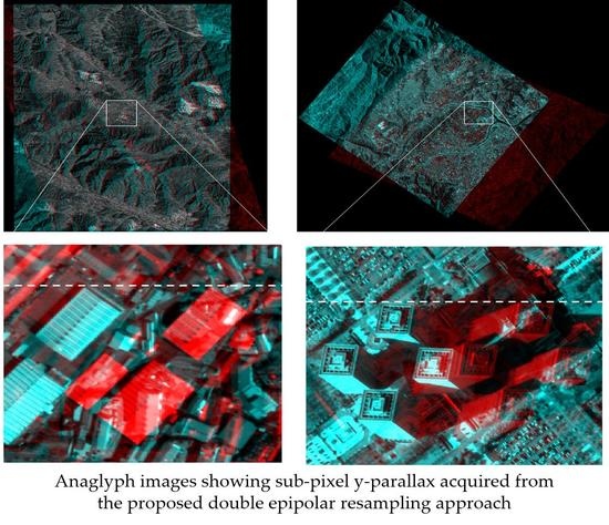
3.5. Fine Epipolar Image Resampling and Y-Parallax Analysis

The extracted conjugate points were transformed back to the original image space and used for RPC bias compensation, called relative orientation. In the step of the coarse epipolar image resampling, we modeled a second order polynomial for the transformation from the original image to the resampled image. By computing the inverse transformation of the second order polynomial, we could transform the conjugate points to the original image space. These conjugate points in the original image space are used for bias-compensation of RPCs.

With bias-compensated RPCs, we performed fine epipolar image resampling and analyzed the y-parallax. Figure 22 shows the y-parallax for along-track Kompsat-3 data. For all methods except Harris, the conjugate points from the coarse epipolar images helped improve the y-parallax in the fine epipolar images. MI and PC provided stable sub-pixel y-parallax for patch size larger than 400 pixels.

Figure 23 presents the y-parallax for across-track Kompsat-3A data. Except in the case of Harris and SURF, the conjugate points from coarse epipolar images helped improve the y-parallax in the fine epipolar images. In the case of Harris and SURF methods, a rather unstable y-parallax was observed. MI and PC provided a stable y-parallax of less than 1 pixel for patch sizes larger than 400 pixels.

In terms of the comparison focusing on the datasets, the across-track dataset showed the better improvement compared to the along-track dataset by applying the proposed method. This result was revealed due to the fact that the general matching methods could work properly in the along-track dataset which shows similar properties between the images. In this case, it would be easier to extract reliable conjugate points even applying the general matching method without applying the double-epipolar resampling method. However, in the case of the across-track dataset that is more challenging to extract reliable conjugate points due to dissimilar properties between the images, the general matching methods are likely to fail to extract reliable conjugate points properly. In this case, the double-epipolar resampling can improve the matching performance significantly while reducing the search space as well as removing the rotation and scale differences that the original images involve.

Figure 24 shows the final anaglyph images of both data with magnified views of the samples. They can be stereo-viewed with anaglyph glasses. The y-parallax was minimized compared to that in the coarse epipolar images.

4. Conclusions

The accurate epipolar resampled images are important for dense matching to reconstruct and display a 3D ground surface. However, RPCs or the sensor models of the stereo data are rather erroneous and not optimal for the reconstruction. In these cases, those errors should be compensated through an orientation process (or bundle adjustment) which requires conjugate points over the images. Therefore, we proposed a double epipolar resampling approach for the robust conjugate point extraction that enables more accurate sensor modeling. The basic idea is that coarse epipolar images with even inaccurate RPCs show better stereo similarity than the original images, thereby allowing better conjugate point extraction. We tested along-track Kompsat-3 stereo data and across-track Kompsat-3A stereo data using four image-matching methods, namely, Harris, SURF, MI, and PC, and compared their performances between the proposed and traditional approaches. Based on the analysis, we conclude that the conjugate point extraction on coarse epipolar images produce more reliable and accurate results instead of the original image case for all the tested matching methods. The accurately extracted conjugate points enabled the fine epipolar image resampling up to sub-pixel accuracy that was not achievable through the traditional approach. The performance increase was more significant for low similarity data such as across-track data.

We drew the following inferences summarized as follows:

• Coarse epipolar images from Kompsat-3/3A data show a large y-parallax of up to 17–25 pixels; this parallax should be minimized for precise 3D mapping.
• Coarse epipolar images allow the extraction of a larger number of conjugate points compared to the original images regardless of the matching methods. Moreover, the transformation models constructed from the conjugate points extracted from coarse epipolar images showed better reliability and accuracy than the ones from the original images.
• Area-based local-template-matching methods, i.e., PC and MI, tended to extract more conjugate points than the feature-based local-template-matching methods such as SURF and Harris. The distribution of the conjugate points was better in the case of the former methods because of the large number of points.
• Given coarse epipolar images, MI and PC with larger patch sizes (>400 pixels) show stable sub-pixel accuracy and y-parallax for along-track and across-track Kompsat-3/3A data.
• Between PC and MI, MI provides more stable results, while PC provides faster results.
• Harris provided quite unstable results in all cases, but SURF provided mixed results of approximately 1–2 pixels in many cases.
• The coarse epipolar image is very helpful for realizing accurate conjugate point extraction. The double epipolar approach showed high effectiveness especially for across-track stereo data for which realizing high stereo consistency is a challenge because of low similarity.

The proposed method showed the advantage of more reliable conjugate point extraction but may have the disadvantage of another epipolar image processing method that requires more processing time. Future studies include further quantitative analysis of similarity increase in the case of the coarse epipolar images compared to the original images. In addition, robust conjugate point extraction methods between heterogeneous data will be investigated.

References

1. Granshaw, S. Photogrammetric terminology: Third edition. Photogramm. Rec. 2016, 31, 210–252. [Google Scholar] [CrossRef]
2. Cho, K.; Wakabayashi, H.; Yang, C.; Soergel, U.; Lanaras, C.; Baltsavias, E.; Rupnik, E.; Nex, F.; Remondino, F. Rapidmap project for disaster monitoring. In Proceedings of the 35th Asian Conference on Remote Sensing (ACRS), Nay Pyi Taw, Myanmar, 27–31 October 2014. [Google Scholar]
3. Tsanis, I.K.; Seiradakis, K.D.; Daliakopoulos, I.N.; Grillakis, M.; Koutroulis, A. Assessment of GeoEye-1 stereo-pair-generated DEM in flood mapping of an ungauged basin. J. Hydroinformatics 2013, 16, 1–18. [Google Scholar] [CrossRef]
4. Rosu, A.-M.; Pierrot-Deseilligny, M.; Delorme, A.; Binet, R.; Klinger, Y. Measurement of ground displacement from optical satellite image correlation using the free open-source software MicMac. ISPRS J. Photogramm. Remote. Sens. 2015, 100, 48–59. [Google Scholar] [CrossRef]
5. Wang, S.; Ren, Z.; Wu, C.; Lei, Q.; Gong, W.; Ou, Q.; Zhang, H.; Ren, G.; Li, C. DEM generation from Worldview-2 stereo imagery and vertical accuracy assessment for its application in active tectonics. Geomorphology 2019, 336, 107–118. [Google Scholar] [CrossRef]
6. Guerin, C.; Binet, R.; Pierrot-Deseilligny, M. Automatic detection of elevation changes by differential DSM analysis: Application to urban areas. IEEE J. Sel. Top. Appl. Earth Obs. Remote. Sens. 2014, 7, 4020–4037. [Google Scholar] [CrossRef]
7. Sohn, G.; Dowman, I. Data fusion of high-resolution satellite imagery and LiDAR data for automatic building extraction. ISPRS J. Photogramm. Remote. Sens. 2007, 62, 43–63. [Google Scholar] [CrossRef]
8. Bi, Q.; Qin, K.; Zhang, H.; Zhang, Y.; Li, Z.; Xu, K. A multi-scale filtering building index for building extraction in very high-resolution satellite imagery. Remote. Sens. 2019, 11, 482. [Google Scholar] [CrossRef] [Green Version]
9. Heipke, C.; Oberst, J.; Albertz, J.; Attwenger, M.; Dorninger, P.; Dorrer, E.; Ewe, M.; Gehrke, S.; Gwinner, K.; Hirschmüller, H.; et al. Evaluating planetary digital terrain models—The HRSC DTM test. Planet. Space Sci. 2007, 55, 2173–2191. [Google Scholar] [CrossRef]
10. Liu, W.C.; Wu, B. An integrated photogrammetric and photoclinometric approach for illumination-invariant pixel-resolution 3D mapping of the lunar surface. ISPRS J. Photogramm. Remote. Sens. 2020, 159, 153–168. [Google Scholar] [CrossRef]
11. Oh, J.; Lee, W.H.; Toth, C.; Grejner-Brzezinska, D.A.; Lee, C. A piecewise approach to epipolar resampling of pushbroom satellite images based on RPC. Photogramm. Eng. Remote. Sens. 2010, 76, 1353–1363. [Google Scholar] [CrossRef]
12. Wang, M.; Hu, F.; Li, J. Epipolar resampling of linear pushbroom satellite imagery by a new epipolarity model. ISPRS J. Photogramm. Remote. Sens. 2011, 66, 347–355. [Google Scholar] [CrossRef]
13. Koh, J.-W.; Yang, H.-S. Unified piecewise epipolar resampling method for pushbroom satellite images. EURASIP J. Image Video Process. 2016, 2016, 314. [Google Scholar] [CrossRef] [Green Version]
14. Fraser, C.S.; Hanley, H.B. Bias-compensated RPCs for sensor orientation of high-resolution satellite imagery. Photogramm. Eng. Remote. Sens. 2005, 71, 909–915. [Google Scholar] [CrossRef]
15. Fraser, C.S.; Ravanbakhsh, M. Georeferencing accuracy of GeoEye-1 imagery. Photogramm. Eng. Remote Sens. 2009, 75, 634–638. [Google Scholar]
16. Oh, J.H.; Lee, C.N. Relative RPCs bias-compensation for satellite stereo images processing. J. Korean Soc. Surv. Geod. Photogramm. Cart. 2018, 36, 287–293. [Google Scholar]
17. Zitová, B.; Flusser, J. Image registration methods: A survey. Image Vis. Comput. 2003, 21, 977–1000. [Google Scholar] [CrossRef] [Green Version]
18. Han, Y.; Byun, Y. Automatic and accurate registration of VHR optical and SAR images using a quadtree structure. Int. J. Remote. Sens. 2015, 36, 2277–2295. [Google Scholar] [CrossRef]
19. Reddy, B.; Chatterji, B. An FFT-based technique for translation, rotation, and scale-invariant image registration. IEEE Trans. Image Process. 1996, 5, 1266–1271. [Google Scholar] [CrossRef] [Green Version]
20. Hu, X.; Zhang, Z.; Tao, C.V. A robust method for semi-automatic extraction of road centerlines using a piecewise parabolic model and least square template matching. Photogramm. Eng. Remote. Sens. 2004, 70, 1393–1398. [Google Scholar] [CrossRef]
21. Huo, C.; Pan, C.; Huo, L.; Zhou, Z. Multilevel SIFT matching for large-size VHR image registration. IEEE Geosci. Remote. Sens. Lett. 2012, 9, 171–175. [Google Scholar] [CrossRef]
22. Yu, L.; Zhang, D.; Holden, E.-J. A fast and fully automatic registration approach based on point features for multi-source remote-sensing images. Comput. Geosci. 2008, 34, 838–848. [Google Scholar] [CrossRef]
23. Lowe, D.G. Distinctive image features from scale-invariant keypoints. Int. J. Comput. Vis. 2004, 60, 91–110. [Google Scholar] [CrossRef]
24. Bay, H.; Ess, A.; Tuytelaars, T.; Van Gool, L. Speeded-Up Robust Features (SURF). Comput. Vis. Image Underst. 2008, 110, 346–359. [Google Scholar] [CrossRef]
25. Leutenegger, S.; Chli, M.; Siegwart, R. BRISK: Binary Robust invariant scalable keypoints. In Proceedings of the 2011 International Conference on Computer Vision, Shanghai, China, 10–12 June 2011; Institute of Electrical and Electronics Engineers (IEEE): Piscataway, NJ, USA, 2011; pp. 2548–2555. [Google Scholar]
26. Hasheminasab, S.M.; Zhou, T.; Habib, A. GNSS/INS-assisted structure from motion strategies for uav-based imagery over mechanized agricultural fields. Remote. Sens. 2020, 12, 351. [Google Scholar] [CrossRef] [Green Version]
27. Habib, A.; Han, Y.; Xiong, W.; He, F.; Zhang, Z.; Crawford, M. Automated ortho-rectification of UAV-based hyperspectral data over an agricultural field using frame RGB imagery. Remote. Sens. 2016, 8, 796. [Google Scholar] [CrossRef] [Green Version]
28. Gong, M.; Zhao, S.; Jiao, L.; Tian, D.; Wang, S. A novel coarse-to-fine scheme for automatic image registration based on SIFT and mutual information. IEEE Trans. Geosci. Remote. Sens. 2014, 52, 4328–4338. [Google Scholar] [CrossRef]
29. Lee, S.R. A coarse-to-fine approach for remote-sensing image registration based on a local method. Int. J. Smart Sens. Intell. Syst. 2010, 3, 690–702. [Google Scholar] [CrossRef] [Green Version]
30. Sedaghat, A.; Mokhtarzade, M.; Ebadi, H. Uniform robust scale-invariant feature matching for optical remote sensing images. IEEE Trans. Geosci. Remote. Sens. 2011, 49, 4516–4527. [Google Scholar] [CrossRef]
31. De Franchis, C.; Meinhardt-Llopis, E.; Michel, J.; Morel, J.-M.; Facciolo, G. An automatic and modular stereo pipeline for pushbroom images. ISPRS Ann. Photogramm. Remote. Sens. Spat. Inf. Sci. 2014, 49–56. [Google Scholar] [CrossRef] [Green Version]
32. Ghuffar, S. Satellite stereo based digital surface model generation using semi global matching in object and image space. In Proceedings of the ISPRS Annals of Photogrammetry, Remote Sensing and Spatial Information Sciences, XXIII ISPRS Congress, Prague, Czech Republic, 12–19 July 2016; pp. 63–68. [Google Scholar]
33. Gong, K.; Fritsch, D. Relative orientation and modified piecewise epipolar resampling for high resolution satellite images. ISPRS Int. Arch. Photogramm. Remote. Sens. Spat. Inf. Sci. 2017, 579–586. [Google Scholar] [CrossRef] [Green Version]
34. El-Mashad, S.Y.; Shoukry, A. Evaluating the robustness of feature correspondence using different feature extractors. In Proceedings of the 2014 19th International Conference on Methods and Models in Automation and Robotics (MMAR), Międzyzdroje, Poland, 2–5 September 2014; Institute of Electrical and Electronics Engineers (IEEE): Piscataway, NJ, USA, 2014; pp. 316–321. [Google Scholar]
35. Tiwari, R.K.; Verma, G.K. A computer vision based framework for visual gun detection using Harris interest point detector. Procedia Comput. Sci. 2015, 54, 703–712. [Google Scholar] [CrossRef] [Green Version]
36. Harris, C.; Stephens, M. A combined corner and edge detector. In Proceedings of the Alvey Vision Conference 1988, Manchester, UK, 31 August–2 September 1988; British Machine Vision Association and Society for Pattern Recognition, 1988; pp. 23–24. [Google Scholar]
37. Alahi, A.; Ortiz, R.; VanderGheynst, P. FREAK: Fast Retina Keypoint. In Proceedings of the 2012 IEEE Conference on Computer Vision and Pattern Recognition, Providence, RH, USA, 16–21 June 2012; Institute of Electrical and Electronics Engineers (IEEE): Piscataway, NJ, USA, 2012; pp. 510–517. [Google Scholar]
38. Han, Y.; Choi, J.; Jung, J.; Chang, A.; Oh, S.; Yeom, J. Automated co-registration of multi-sensor orthophotos generated from unmanned aerial vehicle platforms. J. Sens. 2019, 2019. [Google Scholar] [CrossRef] [Green Version]
39. Baarda, W. A Testing Procedure for Use in Geodetic Networks; Netherlands Geodetic Commission, Publications on Geodesy; New Series; Rijkscommissie voor Geodesie: Delft, The Netherlands, 1968; Volume 2. [Google Scholar]
40. Zhu, Q.; Wu, B.; Xu, Z.-X.; Qing, Z. Seed point selection method for triangle constrained image matching propagation. IEEE Geosci. Remote. Sens. Lett. 2006, 3, 207–211. [Google Scholar] [CrossRef]
41. Han, Y.; Kim, T.; Yeom, J.; Han, Y.; Kim, Y. Improved piecewise linear transformation for precise warping of very-high-resolution remote sensing images. Remote. Sens. 2019, 11, 2235. [Google Scholar] [CrossRef] [Green Version]
Figure 1. Comparison of resampling methods for three-dimensional (3D) mapping: (a) single resampling and (b) double resampling.
Remotesensing 12 02940 g001
Figure 2. Epipolar image resampling (Oh et al., 2010).
Remotesensing 12 02940 g002
Figure 3. Quasi-ground control point (GCP) reconstruction and reprojection.
Remotesensing 12 02940 g003
Figure 4. Test Kompsat-3 along-track stereo images (K3-944 and K3-102) and Kompsat-3A across-track stereo images (K3A-4099, K3A-4025).
Remotesensing 12 02940 g004
Figure 5. Epipolar image resampling of Kompsat-3 along-track stereo images: (a,c) K3-944 (red dots: original image points, blue dots: resampled image points), (b,d) K3-102.
Remotesensing 12 02940 g005
Figure 6. Epipolar image resampling of Kompsat-3A across-track stereo images: (a,c) K3A-4099 (red dots: original image points, blue dots: resampled image points), (b,d) K3A-4205.
Remotesensing 12 02940 g006
Figure 7. Y-parallax in the coarse epipolar resampled images: (a) along-track Kompsat-3 epipolar and (b) across-track Kompsat-3A epipolar.
Remotesensing 12 02940 g007
Figure 8. Results of conjugate point extraction (along-track Kompsat-3 stereo data): (a,b) number of conjugate points, (c,d) distribution quality, (e,f) correlation coefficient (g,h) process times in original and coarse epipolar images, respectively.
Remotesensing 12 02940 g008
Figure 9. Results of matching point extraction (across-track Kompsat-3A stereo data): (a,b) number of conjugate points, (c,d) distribution quality, (e,f) correlation coefficient (g,h) process times in original and coarse epipolar images, respectively.
Remotesensing 12 02940 g009
Figure 10. Matching results of Kompsat-3 along-track stereo images (template size: 500 × 500 pixels): (a) number of extracted conjugate points, (b) distribution quality, (c) correlation coefficient, and (d) acquisition time.
Remotesensing 12 02940 g010
Figure 11. Visual expression of the extracted conjugate points overlaid on K3-944 image (template size: 500 × 500 pixels): (a) phase correlation (PC), (b) mutual information (MI), (c) speeded up robust features (SURF), and (d) HARRIS–fast retina keypoint (FREAK) applied to the original image, and (e) PC, (f) MI, (g) SURF, and (h) HARRIS–FREAK applied to the coarse epipolar image.
Remotesensing 12 02940 g011
Figure 12. Matching results of Kompsat-3A across-track stereo images (template size: 500 × 500 pixels): (a) number of extracted conjugate points, (b) distribution quality, (c) correlation coefficient, and (d) acquisition time.
Remotesensing 12 02940 g012
Figure 13. Visual expression of the extracted conjugate points overlaid with K3A-4099 image (template size: 500 × 500 pixels): (a) PC, (b) MI, (c) SURF, and (d) HARRIS–FREAK applied to the original image, and (e) PC, (f) MI, (g) SURF, and (h) HARRIS–FREAK applied to the coarse epipolar image.
Remotesensing 12 02940 g013
Figure 14. Reprojection errors (along-track Kompsat-3 original—before adjustment): (a) HARRIS–FREAK (b) SURF, (c) MI, and (d) PC.
Remotesensing 12 02940 g014
Figure 15. Reprojection errors (along-track Kompsat-3 coarse epipolar—before adjustment): (a) HARRIS–FREAK (b) SURF, (c) MI, and (d) PC.
Remotesensing 12 02940 g015
Figure 16. Reprojection errors (across-track Kompsat-3A original—before adjustment): (a) HARRIS–FREAK (b) SURF, (c) MI, and (d) PC.
Remotesensing 12 02940 g016
Figure 17. Reprojection errors (across-track Kompsat-3A coarse epipolar—before adjustment): (a) HARRIS–FREAK (b) SURF, (c) MI, and (d) PC.
Remotesensing 12 02940 g017
Figure 18. Reprojection errors (along-track Kompsat-3 original—after adjustment): (a) HARRIS–FREAK (b) SURF, (c) MI, and (d) PC.
Remotesensing 12 02940 g018
Figure 19. Reprojection errors (along-track Kompsat-3 coarse epipolar—after adjustment): (a) HARRIS–FREAK (b) SURF, (c) MI, and (d) PC.
Remotesensing 12 02940 g019
Figure 20. Reprojection errors (across-track Kompsat-3A original—after adjustment): (a) HARRIS–FREAK (b) SURF, (c) MI, and (d) PC.
Remotesensing 12 02940 g020
Figure 21. Reprojection errors (across-track Kompsat-3A coarse epipolar—after adjustment): (a) HARRIS–FREAK (b) SURF, (c) MI, and (d) PC.
Remotesensing 12 02940 g021
Figure 22. Y-parallax (along-track Kompsat-3): (a) HARRIS–FREAK (b) SURF, (c) MI, and (d) PC.
Remotesensing 12 02940 g022
Figure 23. Y-parallax (across-track Kompsat-3A): (a) HARRIS–FREAK (b) SURF, (c) MI, and (d) PC.
Remotesensing 12 02940 g023
Figure 24. Final anaglyph images showing sub-pixel y-parallax (a) along-track Kompsat-3 and (b) across-track Kompsat-3A.
Remotesensing 12 02940 g024