Article

Increasing Historical Tropical Cyclone-Induced Extreme Wave Heights in the Northern East China Sea during 1979 to 2018

1
Key Laboratory of Ocean Circulation and Waves, Institute of Oceanology, Chinese Academy of Sciences, Qingdao 266071, China
2
Laboratory for Ocean and Climate Dynamics, Qingdao National Laboratory for Marine Science and Technology, Qingdao 266237, China
3
Center for Ocean Mega-Science, Chinese Academy of Sciences, Qingdao 266071, China
4
Hubei Key Laboratory of Marine Geological Resources, China University of Geosciences, Wuhan 430074, China
5
Chinese Academy of Sciences, Beijing 100049, China
6
Center for High Performance Computing and System Simulation, Pilot National Laboratory for Marine Science and Technology Laboratory for Ocean and Climate Dynamics, Qingdao National Laboratory for Marine Science and Technology, Qingdao 266237, China
*
Author to whom correspondence should be addressed.
Remote Sens. 2020, 12(15), 2464; https://doi.org/10.3390/rs12152464
Submission received: 21 July 2020 / Revised: 28 July 2020 / Accepted: 29 July 2020 / Published: 31 July 2020
(This article belongs to the Special Issue Coastal Environments and Coastal Hazards)

Abstract

:
Tropical cyclone (TC)-induced wind waves are a major concern in coastal safety, therefore quantifying the long-term change in extreme TC waves is critical for the design of coastal infrastructures and for understanding variations in coastal morphology. In this study, a trend analysis is performed on the TC-induced extreme wave heights in the northern East China Sea using numerically simulated wave height data during the period of 1979 to 2018. The simulation was forced with historical TC winds constructed using a parametric TC wind model with satellite-observed TC best-track data as the input. The results show consistently increasing extreme wave heights throughout the study region, which are induced predominantly by the increasing TC intensity. The increase rates (0.01–0.08 m yr−1) are relatively large (small) in offshore (nearshore) waters and at relatively high (low) latitudes. The spatial variability of the wave height trend is highly sensitive to the type of TC track. An analytical model of extreme wave height trend is developed that can efficiently estimate the rate of change in the extreme wave heights using extreme wind speed information.

1. Introduction

Extreme high wind waves generated by tropical cyclone (hereafter TC) conditions are of great importance for many marine applications (e.g., coastal engineering, safety, ecosystems, and morphology changes). TCs are generated in tropical regions and then move toward higher latitudes. The northern East China Sea (ECS), a marginal sea located in the western North Pacific Ocean, is the region with the most frequent TC activity [1]. It was reported that 41 TCs passed through the northern ECS over the past 40 years (1979 to 2018, as shown in Figure 1). The northern ECS is characterized by a wide continental shelf with water depths generally shallower than 200 m. The northern ECS consists of an inner gulf named the Bohai Sea and an outer gulf called the Yellow Sea. The two seas are separated by an open boundary between the Liaodong Peninsula and Shandong Peninsula (Figure 1). TCs pose huge threats to the coastal regions along the northern ECS, as they can result in losses of life, property, and habitat. From 2014 to 2018 alone, disasters from cyclone-induced waves caused direct economic losses of CN¥ 41.437 million (~5.945 million US dollars) and 14 deaths in China’s coastal provinces of the Yellow Sea and the Bohai Sea.
Monitoring and understanding the changes in extreme winds and waves have long constituted important research topics. The long-term increase in western Pacific TC intensity over the past decades, which has been widely reported in the literature, is largely attributed to upper-ocean warming under global climate change [2,3,4]. Guan et al. [5] suggested that the percentage of TCs that make landfall over East and Southeast Asia, as well as their landfall intensities, have increased during the past 40 years, thus increasing the threat of coastal hazards associated with extreme wind-waves and storm surges [6,7]. Hence, quantifying the long-term change in extreme TC waves is critical for the design of coastal infrastructure and for understanding variations in coastal morphology.
Extreme wave climate variability under a warming climate has been the subject of many investigations [8,9,10]. Most of these studies were based on either satellite altimetry measurements or wave reanalysis data. However, neither type of data is ideal for the analysis of extreme TC wind waves: altimeters under-sample extreme wave events, and thus tend to underestimate extreme wave heights (e.g., 99th percentile) at a given location [6]; although numerical wave models are efficient in reproducing the extreme wave field during a TC event, wave reanalysis data also tend to underestimate extreme wave heights. This is mainly because the extreme wind conditions are often underrepresented in the wave reanalysis that drives the numerical wave models [11].
TC information, including time, position, and central pressure, has been routinely observed by satellite since 1969/1970 and is typically referred to as TC best-track data. Wind parametric models using TC best-track data were demonstrated to well reproduce the TC wind fields during TC events, and they were widely used in the simulation of TC wind waves [12,13]. Recently, Wang et al. [14] performed a numerical study of wind waves during three TC events in the northern ECS; the wind field was constructed using the Holland parametric model [15] with TC best-track data as the input, and the simulated wind speeds and wave heights were both in good agreement with in-situ measurements.
In this study, the historical change in the TC-induced extreme wind waves in the northern ECS, during the period 1979 to 2018, was analyzed. TC wave data were simulated by a tightly coupled SWAN + ADCIRC (simulating waves nearshore + advanced circulation) model forced by a constructed wind field from the Holland parametric TC wind model and satellite-observed TC best tracks. The simulation covered the four decades from 1979 to 2018. The remainder of this paper is organized as follows: in Section 2, the parametric TC wind model and coupled numerical model (SWAN + ADCIRC) are described. In Section 3, the spatial distribution and long-term trends of extreme wave heights and wind speeds are presented, and their interrelationships are examined. Discussions and conclusions are presented in Section 4.

2. Methods

2.1. Parametric TC Wind Simulation

Parametric models have been widely used to construct TC wind fields, greatly advancing the study of storm wave and surge forecasts and coastal risk analysis [16,17]. Several notable parametric models have been proposed, such as Holland [15], Jelesnianski and Taylor [18], Willoughby et al. [19], and Emanuel and Rotunno [20]. Krien et al. [21] assessed the performance of these parametric models using satellite data and reported no preference for a certain parametric model in all cases.
Wang et al. [14] applied the Holland parametric model to construct the wind fields during three TC events in the ECS. The results suggested that the constructed winds compare well with those measured by in-situ buoys when the undetermined parameters, namely the radius of the maximum wind speed (Rmax) and the shape parameter (Bs), are suitably configured. Observational evidence has been reported supporting that both Rmax and Bs show correlations with central pressure, but their relationships vary among different regions [22,23,24,25]. The results of Wang et al. [14] show that the Rmax formulation proposed by Jiang et al. [25] and the Bs formulation given by Powell et al. [23] achieved the best scores in the construction of TC wind fields in the ECS. Because the parametric model is static and the wind field is symmetric, the movements of TCs need to be considered to obtain the wind field asymmetry. Wind products from the climate forecast system reanalysis (CFSR) were used as the background wind speed and were blended into the parametric TC wind model for the numerical simulation. The detailed procedures can be found in Wang et al. [14].
As an input in the TC parametric model, TC best-track data were acquired from the Shanghai Typhoon Institute of the China Meteorological Administration (CMA-STI) Best Track Dataset for Tropical Cyclones in the Western North Pacific (www.typhoon.org.cn), which contains various types of TC information, including their time, position, pressure, and intensity [26]. The TC tracks (Figure 1) can be classified into two types based on whether the TC made landfall before entering the northern ECS, the first type (TC_T1) does not make landfall on the mainland before entering the Yellow Sea while the second type (TC_T2) does. The numbers of the two types are comparable. In total, 24 TC_T1 and 17 TC_T2 occurred from 1979 to 2018.
The statistics of the TCs are summarized in Figure 2. There is no noticeable trend in the annual occurrence of TCs, and the yearly distribution of TCs appear quite random: there were 11 years in which more than one TC occurred and 13 years in which no TCs occurred, and four TCs occurred in 1985. These TCs appeared from June to September, and more than 40% of them were in July. These TCs were also classified based on their intensity scale using the Chinese National Standard for the Grade of Tropical Cyclones (GB/T 19201–2006) based on the 2-min sustained maximum wind speed: tropical depression (TD, 10.8–17.1 m s−1); tropical storm (TS, 17.2–24.4 m s−1); severe tropical storm (STS, 24.5–32.6 m s−1); and typhoon (TY, 32.7–41.4 m s−1). The TCs in the dataset range from tropical depressions to severe tropical storms, and tropical depressions are dominant (>60%).

2.2. Coupled Wave-Circulation Simulation

In addition to wind forcing, wind waves can be strongly modulated by the spatial gradient of the current under TC conditions [27,28]. Wind waves are also extremely sensitive to changes in water level (depth) induced by storm tides [16]. Taking these effects into consideration, we employ the tightly coupled SWAN + ADCIRC model [29] to simulate cyclone waves from deep water to coastal regions in the northern ECS. The coupled model allows wave-circulation interactions to be solved on the same unstructured mesh, resulting in a more accurate and efficient solution. The computational mesh was developed to cover the entire northern ECS using the mesh generation module of the surface-water modeling system (SMS). The grid consisted of an unstructured triangular mesh with 49,094 nodes and 95,682 elements. The mesh resolutions range from 500 m in coastal regions to 10 km along the open boundaries. The bathymetry used in the model was the ETOPO1 (http://www.ngdc.noaa.gov/mgg/global/global.html) dataset, and the nearshore depths were obtained from nautical charts provided by the Compass Department of the Chinese Admiralty.
The SWAN model is a spectral wave model that can effectively simulate the generation, propagation, and dissipation of surface waves. SWAN solves the wave action balance equation to calculate the wave action density and thus the phase-averaged wave characteristics. This equation was solved in both the geographic and spectral domains, in which the source and sink terms are included to represent various physical processes. In deep water, the growth of the wave height is controlled mainly by the relative importance of the wind input and whitecapping dissipation, whereas in shallow water, wave growth is further modulated and dissipated by bottom friction. SWAN provides several physical solutions to account for these physical processes. Wang et al. [14] analyzed the influences of available physical solutions on TC-induced wave simulations and found that the differences among these solutions were nonnegligible. The performances of these solutions were assessed by comparing the simulated results with in situ buoy measurements, and the results indicated that the best performance arose when using the wind input and whitecapping dissipation model developed by Komen et al. [30] and the bottom friction model by Hasselmann et al. [31]. The same model configuration was employed here for the historical TC wave simulation. The other terms and parameters were applied with the default settings and values, and the time step in SWAN was set to 10 min.
ADCIRC is a circulation model that has been widely applied to solve free surface circulation and transport problems [17,32]. ADCIRC solves the depth-averaged barotropic form of the shallow water equation for the water level and momentum. The depth-integrated currents are solved in the vertically integrated momentum equations. In this study, the model was driven by the harmonic constants of eight main astronomical tide components (M2, S2, N2, K2, K1, O1, P1, and Q1) at the open boundaries, and the constants were obtained from the Tidal Prediction Software developed by Oregon State University. The computational time step was set to 1 s to satisfy the Courant–Friedrichs–Lewy stability condition. The wind drag coefficient was calculated using the formula developed by Garratt [33], which is linearly related to the wind speed, and the maximum limit for the wind drag coefficient was set to 0.0025.
The coupling between SWAN and ADCIRC was leveraged in two ways to account for the effects of the wave–current interaction and wave–tide interaction: the wave-induced radiation stress gradient was fed back into ADCIRC to influence the water level, and the current and water level were fed back into SWAN. More details on the coupling process can be found in Dietrich et al. [29]. SWAN and ADCIRC exchange data every 10 min. The coupled SWAN + ADCIRC model was run in cold-start mode. The model was forced with background wind (CFSR) 2 days prior to a TC entering the computation area. The outputs of the model spanned the period of the TC entering the computation area.
The model was validated by Wang et al. [14,34] through comparisons with in-situ buoy measurements located in China’s coastal waters (provided by Marine Scientific Data Center, Institute of Oceanology, Chinese Academy of Sciences), in which five TC events (TC Damrey in 2012, TC Fung-wong in 2014, TC Chan-hom in 2015, TC Muifa in 2011, and TC Lekima in 2019) were considered. Their simulation indicated that the coupled model can effectively reproduce TC wave heights from offshore deep waters to nearshore shallow water regions, with relative errors (the ratio between the bias and mean) generally within a magnitude of ~5%.

3. Results

3.1. Distribution of Extreme Wave Height and Wind Speed

The analysis focused on extreme significant wave height (SWH) in terms of the annual upper percentile values. As is commonly used in the literature [9], the annual 90th percentile SWH (H90) was selected for analysis. The corresponding wind values (90th percentile values of U10, hereafter U90) were also given as a reference.
Figure 3a,b shows the multiyear maximum values of H90 and U90. H90 (U90) decreases from over 8 m (25 m/s) in the south of the Yellow Sea to less than 3 m (13 m/s) in the Bohai Sea. The variation in the wave height with latitude appears to be more significant than the variation in the wind speed, which was expected from the fact that both the wind fetch and the water depth decrease toward high latitudes.
The extreme values of the wind speed and wave height corresponding to the two TC types are shown in Figure 3c–f. There are clear differences in the spatial distributions between the two types. For TC_T1, both maximum wind speeds and wave heights occurred in the eastern part of the Yellow Sea, however, the wind speeds and wave heights in the Bohai Sea were quite small. The situation is reversed for TC_T2, for which high wind speeds and wave heights occurred on the west coast of the Yellow Sea, and the wave heights in the Bohai Sea were larger than those of TC_T1. Generally, extreme waves were induced predominantly by TC_T1 in the Yellow Sea except on the west coast, while TC_T2 contributed significantly to the extreme values in the Bohai Sea and the west coast of the Yellow Sea.

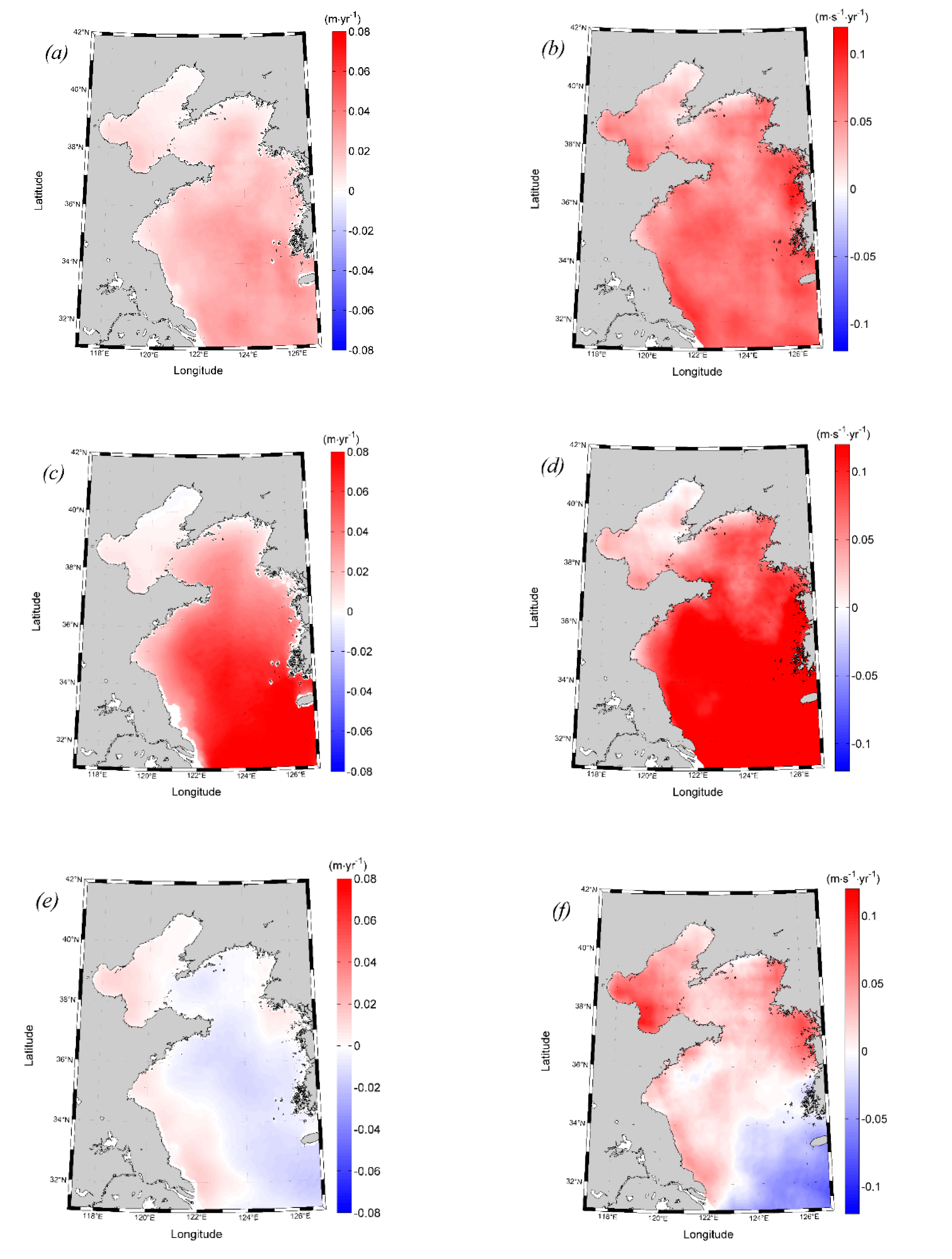
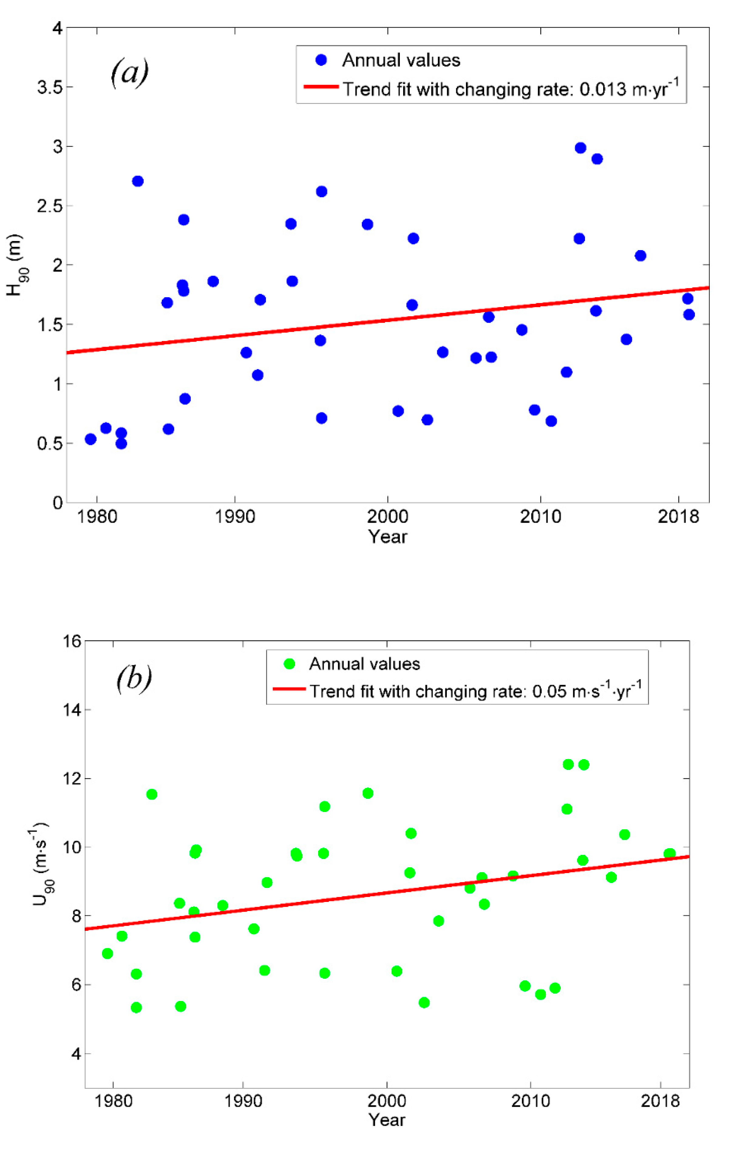
3.2. Trends of Extreme Wave Height and Wind Speed

The long-term trends of H90 and U90 are illustrated in Figure 4. The corresponding changing rates were derived using the linear fit and Mann–Kendall test, and the difference between them was found to be indiscernible; thus, only the results from the linear fit were considered. Both H90 and U90 exhibit an increasing trend throughout the whole region, and the rate of increase in H90 (U90) generally decreases with increasing latitude, varying in the range of 0.01–0.07 m yr−1 (0.01–0.12 m s−1 yr−1). With respect to the two TC types, significant increasing trends of H90 and U90 are observed throughout the Yellow Sea for TC_T1. For TC_T2, increasing trends of H90 and U90 are observed in the Bohai Sea and the west coast of the Yellow Sea, but a decreasing trend of H90 is observed in the eastern Yellow Sea.
The temporal variations in spatially averaged H90 and U90 are plotted in Figure 5a,b, respectively. The TC duration is also given in Figure 5c because this parameter is important for considering ocean dynamics [5]. All three parameters show an increasing trend: H90, U90, and the TC duration increases at rates of 0.013 m yr−1, 0.05 m s−1 yr−1, and 0.25 h yr−1, respectively. The correlation coefficient (CC) between H90 and U90 in Figure 5 reaches 0.88 but is only 0.24 between H90 and the TC duration. These results indicate that the increasing trend of the extreme wave height may be attributable to the increasing TC intensity.

3.3. Relation Between the Extreme Wind Speed and Wave Height Trends

As illustrated above, the spatial distributions of H90 and U90 and their trends exhibit similarities. This can be attributed to the strong wind-wave interaction under TC conditions [35,36]. The CC between the hourly SWH and wind speed on each grid point was estimated, and it was found that 98% of the grid points have a CC higher than 0.9, implying strong wind-wave coupling effects. Therefore, the trend of H90 can be directly linked to the trend of U90.
For a wind wave, an exponential relation between the wave height (H) and wind speed (U) is suggested [37]:
H = A U B
where A and B are coefficients that depend on the development stage of wind waves associated with the fetch, duration, and water depth in shallow waters. B typically lies in the range of 1–2.
Similarly, we assumed that the exponential relation is valid for H90 and U90:
H 90 = a i U 90 b i         i = 1 , 2 , . . n
where ai and bi are coefficients at a given grid point i and where the coefficients are assumed to spatially vary depending on the factors that influence the growth of wind waves, including the fetch, duration, and water depth; n is the total number of grids. The logarithmic least-square method is used to estimate ai and bi.
Additionally, we assumed that the temporally averaged H90 and U90 satisfy the following relation:
H 90 ¯ = a i U 90 ¯ b i
where the overbar denotes a long-term averaged value.
Considering the temporal variations in H90 and U90, the following relation is derived:
H 90 ¯ + Δ H 90 = a i ( U 90 ¯ + Δ U 90 ) b i
Dividing Equation (4) by Equation (3), the following is obtained:
1 + Δ H 90 / H 90 ¯ = ( 1 + Δ U 90 / U 90 ¯ ) b i
Since the magnitude of Δ U 90 is much smaller than that of U 90 ¯ , Equation (5) can be approximated as follows:
Δ H 90 / H 90 ¯ b i Δ U 90 / U 90 ¯
The result indicates that the relative changes in wave height and wind speed are linearly related to a proportion coefficient of bi.
Based on Equations (3) and (6), the rate of change in H90 and U90 can be derived from wind speed information:
Δ H 90 a i b i U 90 ¯ ( b i - 1 ) Δ U 90
We plotted H90 trends from the numerical model against those from Equation (7) in Figure 6. A generally consistent result was observed, with a relative bias of 0.03, and a CC of 0.90.

4. Discussions and Conclusions

We performed a 40-year numerical simulation of TC-induced wind waves using a tightly coupled SWAN+ADCIRC model specifically configured for the northern ECS. A trend analysis was performed on the extreme wave heights and wind speeds using the simulated data. The results showed that both extreme wave heights and wind speeds consistently increased during the period of 1979 to 2018 in the northern ECS. Recently, Li et al. [6] analyzed the trends of extreme wave heights in China’s coastal seas during the period of 1992 to 2010 based on a combined analysis of numerical simulations and satellite altimetry observations. Their results also indicated increasing extreme wave heights throughout the northern ECS, but the increase rates were generally smaller (0–0.06 m yr−1) than those in this study. Several reasons can account for this difference: first, [6] used the 99th-percentile wave height rather than the 90th-percentile high wave height used in this study; second, their extreme values were not restricted to TC-induced wind waves, so that other extreme weather events, such as cold waves and extratropical cyclones may also contribute; third, the periods of interest were different in the two studies. Despite these differences, both studies showed significant increasing trends in extreme wave heights in the northern ECS, and their spatial distributions of trends were in good agreement.
The rates of change in the extreme wave heights were relatively large (small) in the offshore (nearshore) region and low (high) latitudes. The spatial variability of extreme wind speed and wave height trends is found to be critically dependent on the TC track: the increases in extreme wind speed and wave height in the Yellow Sea, especially in the East Yellow Sea, are caused predominantly by TC_T1, while TC_T2 contributes to the increasing trend along the western coastal regions. The increasing trends by TC_T1 are overall more significant than those by TC_T2, which can be explained by the fact that TC intensity of the type TC_T2 is smaller because they suffer from land dissipation.
The increasing wave height trends can be attributed mainly to the increasing TC intensity over the studied period. The TC intensity in the western North Pacific is projected to increase during the 21st century due to the warming climate [38], and a similar trend is thus expected for the TC-induced wave height. An analytical extreme wave height trend model, which can provide robust trend estimates using extreme wind speed information, is developed. Compared to the numerical simulation, this method can fast project future changes in TC-induced extreme wave height with low computational costs.

Author Contributions

Conceptualization, S.L. and Y.H.; Methodology, S.L., N.W., and J.L.; Investigation, S.L. and H.J.; All authors contributed to the writing. All authors have read and agreed to the published version of the manuscript.

Funding

This work is supported by the National Natural Science Foundation of China, grant number U1706216, 41976010, 41806010, the CAS Strategic Priority Project, grant number XDA19060202, the National Key Research and Development Program of China, grant number 2016YFC1402000, 2017YFC1404101, and the Open Fund Project of Key Laboratory of Marine Environmental Information Technology. The numerical work is supported by the High-Performance Computing Center, Institute of Oceanology, Chinese Academy of Sciences, China.

Conflicts of Interest

The authors declare no conflict of interest.

References

  1. Peduzzi, P.; Chatenoux, B.; Dao, H.; De Bono, A.; Herold, C.; Kossin, J.P.; Mouton, F.; Nordbeck, O. Global trends in tropical cyclone risk. Nat. Clim. Chang. 2012, 2, 289–294. [Google Scholar] [CrossRef]
  2. Webster, P.J.; Holland, G.J.; Curry, J.A.; Chang, H.-R. Changes in tropical cyclone number, duration, and intensity in a warming environment. Science 2005, 309, 1844–1846. [Google Scholar] [CrossRef] [PubMed] [Green Version]
  3. Emanuel, K. Increasing destructiveness of tropical cyclones over the past 30 years. Nature 2005, 436, 686–688. [Google Scholar] [CrossRef] [PubMed]
  4. Mei, W.; Xie, S.-P.; Primeau, F.; McWilliams, J.C.; Pasquero, C. Northwestern Pacific typhoon intensity controlled by changes in ocean temperatures. Sci. Adv. 2015, 1, e1500014. [Google Scholar] [CrossRef] [PubMed] [Green Version]
  5. Guan, S.; Li, S.; Hou, Y.; Hu, P.; Liu, Z.; Feng, J. Increasing threat of landfalling typhoons in the western North Pacific between 1974 and 2013. Int. J. Appl. Earth Obs. Geoinf. 2018, 68, 279–286. [Google Scholar] [CrossRef]
  6. Li, S.; Guan, S.; Hou, Y.; Liu, Y.; Bi, F. Evaluation and adjustment of altimeter measurement and numerical hindcast in wave height trend estimation in China’s coastal seas. Int. J. Appl. Earth Obs. Geoinf. 2018, 67, 161–172. [Google Scholar] [CrossRef]
  7. Feng, X.; Li, M.; Yin, B.; Yang, D.; Yang, H. Study of storm surge trends in typhoon-prone coastal areas based on observations and surge-wave coupled simulations. Int. J. Appl. Earth Obs. Geoinf. 2018, 68, 272–278. [Google Scholar] [CrossRef]
  8. Izaguirre, C.; Mendez, F.J.; Menéndez, M.; Luceño, A.; Losada, I.J. Extreme wave climate variability in southern Europe using satellite data. J. Geophys. Res. Space Phys. 2010, 115, 04009. [Google Scholar] [CrossRef]
  9. Young, I.R.; Zieger, S.; Babanin, A. Global Trends in Wind Speed and Wave Height. Science 2011, 332, 451–455. [Google Scholar] [CrossRef]
  10. Zhang, C.K. Estimation of long-term wave statistics in the East China Sea. J. Coast. Res. 2013, 65, 177–182. [Google Scholar]
  11. Stephens, S.A.; Gorman, R. Extreme wave predictions around New Zealand from hindcast data. N. Z. J. Mar. Freshw. Res. 2006, 40, 399–411. [Google Scholar] [CrossRef]
  12. Xu, F.; Perrie, W.; Toulany, B.; Smith, P.C. Wind-generated waves in Hurricane Juan. Ocean Model. 2007, 16, 188–205. [Google Scholar] [CrossRef]
  13. Liu, H.; Xie, L.; Pietrafesa, L.J.; Bao, S. Sensitivity of wind waves to hurricane wind characteristics. Ocean Model. 2007, 18, 37–52. [Google Scholar] [CrossRef]
  14. Wang, N.; Hou, Y.; Li, S.; Li, R. Numerical simulation and preliminary analysis of typhoon waves during three typhoons in the Yellow Sea and East China Sea. J. Oceanol. Limnol. 2019, 37, 1805–1816. [Google Scholar] [CrossRef]
  15. Holland, G.J. An Analytic Model of the Wind and Pressure Profiles in Hurricanes. Mon. Weather. Rev. 1980, 108, 1212–1218. [Google Scholar] [CrossRef]
  16. Feng, X.; Yin, B.; Yang, D. Development of an unstructured-grid wave-current coupled model and its application. Ocean Model. 2016, 104, 213–225. [Google Scholar] [CrossRef]
  17. Wang, K.; Hou, Y.; Li, S.; Du, M.; Chen, J.; Lu, J. A comparative study of storm surge and wave setup in the East China Sea between two severe weather events. Estuar. Coast. Shelf Sci. 2020, 235, 106583. [Google Scholar] [CrossRef]
  18. Jelesnianski, C.P.; Taylor, A.D. A Preliminary View of Storm Surges before and after Storm Modifications NOAA, Technical Memorandum, ERL WMPO-3; Environmental Research Laboratories, Weather Modification Program Office: Boulder, CO, USA, 1973; Volume 3, p. 33. [Google Scholar]
  19. Willoughby, H.E.; Darling, R.W.R.; Rahn, M.E. Parametric representation of the primary hurricane vortex. part II: A new family of sectionally continuous profiles. Mon. Weather. Rev. 2006, 134, 1102–1120. [Google Scholar] [CrossRef] [Green Version]
  20. Emanuel, K.; Rotunno, R. Self-stratification of tropical cyclone outflow. Part I: Implications for storm structure. J. Atmos. Sci. 2011, 68, 2236–2249. [Google Scholar] [CrossRef]
  21. Krien, Y.; Arnaud, G.; Cécé, R.; Ruf, C.; Belmadani, A.; Khan, J.U.; Bernard, D.C.; Islam, A.; Durand, F.; Testut, L.; et al. Can We Improve Parametric Cyclonic Wind Fields Using Recent Satellite Remote Sensing Data? Remote Sens. 2018, 10, 1963. [Google Scholar] [CrossRef] [Green Version]
  22. Vickery, P.J.; Masters, F.J.; Powell, M.; Wadhera, D. Hurricane hazard modeling: The past, present, and future. J. Wind Eng. Ind. Aerodyn. 2009, 97, 392–405. [Google Scholar] [CrossRef]
  23. Powell, M.; Soukup, G.; Cocke, S.; Gulati, S.; Morisseau-Leroy, N.; Hamid, S.; Dorst, N.; Axe, L. State of Florida hurricane loss projection model: Atmospheric science component. J. Wind Eng. Ind. Aerodyn. 2005, 93, 651–674. [Google Scholar] [CrossRef] [Green Version]
  24. Graham, H.E. Meteorological Considerations Pertinent to Standard Project Hurricane, Atlantic and Gulf Coasts of the United States; U.S. Department of Commerce, Weather Bureau: Washington, DC, USA, 1959.
  25. Jiang, Z.H.; Hua, F.; Qu, P. A new scheme for adjusting the tropical cyclone parameters. Adv. Mar. Sci. 2008, 26, 1–7, (in Chinese with English abstract). [Google Scholar]
  26. Ying, M.; Zhang, W.; Yu, H.; Lu, X.; Feng, J.; Fan, Y.; Zhu, Y.; Chen, D. An Overview of the China Meteorological Administration Tropical Cyclone Database. J. Atmos. Ocean. Technol. 2014, 31, 287–301. [Google Scholar] [CrossRef] [Green Version]
  27. Wang, P.; Sheng, J. A comparative study of wave-current interactions over the eastern Canadian shelf under severe weather conditions using a coupled wave-circulation model. J. Geophys. Res. Oceans 2016, 121, 5252–5281. [Google Scholar] [CrossRef]
  28. Mao, M.; Xia, M. Dynamics of wave–current–surge interactions in Lake Michigan: A model comparison. Ocean Model. 2017, 110, 1–20. [Google Scholar] [CrossRef] [Green Version]
  29. Dietrich, J.C.; Zijlema, M.; Westerink, J.; Holthuijsen, L.; Dawson, C.N.; Luettich, R.A.; Jensen, R.E.; Smith, J.M.; Stelling, G.; Stone, G.W. Modeling hurricane waves and storm surge using integrally-coupled, scalable computations. Coast. Eng. 2011, 58, 45–65. [Google Scholar] [CrossRef]
  30. Komen, G.J.; Hasselmann, K. On the existence of a fully developed wind-sea spectrum. J. Phys. Oceanogr. 1984, 14, 1271–1285. [Google Scholar] [CrossRef]
  31. Hasselmann, K.; Barnett, T.P.; Bouws, E.; Carlson, H.; Cartwright, D.E.; Enke, K.; Ewign, J.A.; Gienapp, H.; Hasselmann, D.E.; Kruseman, P.; et al. Measurements of wind-wave growth and swell decay during the Joint North Sea Wave Project (JONSWAP). Dtsch. Hydrogr. Z. 1973, 12, 1–95. [Google Scholar]
  32. Bilskie, M.V.; Hagen, S.C.; Medeiros, S.C.; Cox, A.T.; Salisbury, M.; Coggin, D. Data and numerical analysis of astronomic tides, wind-waves, and hurricane storm surge along the northern Gulf of Mexico. J. Geophys. Res. Oceans 2016, 121, 3625–3658. [Google Scholar] [CrossRef]
  33. Garratt, J.R. Review of drag coefficients over oceans and continents. Mon. Weather Rev. 1977, 105, 915–929. [Google Scholar] [CrossRef] [Green Version]
  34. Wang, N.; Hou, Y.; Li, S.; Mo, D.; Li, J. Numerical simulation of the hazard distribution of typhoon waves in 1979—2018. J. Oceanol. Limnol. 2020, 51, 525–532, (in Chinese with English abstract). [Google Scholar]
  35. Young, I.R. Directional spectra of hurricane wind waves. J. Geophys. Res. Space Phys. 2006, 111, C8. [Google Scholar] [CrossRef]
  36. Xu, Y.; He, H.; Song, J.; Hou, Y.; Li, F. Observations and Modeling of Typhoon Waves in the South China Sea. J. Phys. Oceanogr. 2017, 47, 1307–1324. [Google Scholar] [CrossRef]
  37. The WAMDI Group. The WAM model: A third generation ocean wave prediction model. J. Phys. Oceanogr. 1988, 18, 1775–1810. [Google Scholar] [CrossRef] [Green Version]
  38. Emanuel, K. Downscaling CMIP5 climate models shows increased tropical cyclone activity over the 21st century. Proc. Natl. Acad. Sci. USA 2013, 110, 12219–12224. [Google Scholar] [CrossRef] [PubMed] [Green Version]
Figure 1. The northern East China Sea and the TC tracks (light blue lines, the crosses in the line are the six-hourly TC locations). The red line is the dividing line between the Bohai Sea and the Yellow Sea. The red arrows are schematic tracks for TC_T1, and the dark blue arrows are schematic tracks for TC_T2.
Remotesensing 12 02464 g001
Figure 2. Statistics of TCs: (a) TC numbers over the year; (b) occurrence month; (c) intensity scale.
Remotesensing 12 02464 g002
Figure 3. Spatial distributions of the multiyear maximum H90 ((a), all cases; (c), cases of TC_T1; (e), cases of TC_T2) and U90 ((b), all cases; (d), cases of TC_T1; (f), cases of TC_T2).
Remotesensing 12 02464 g003
Figure 4. Spatial distributions of the trends in H90 ((a), all cases; (c) cases of TC_T1; (e) cases of TC_T2) and U90 ((b), all cases; (d) cases of TC_T1; (f) cases of TC_T2).
Remotesensing 12 02464 g004
Figure 5. Annual variations of spatially averaged parameters: (a) H90, (b) U90, and (c) TC duration.
Remotesensing 12 02464 g005aRemotesensing 12 02464 g005b
Figure 6. Comparisons of the H90 trends derived from the numerical simulation and the analytical model of Equation (7). The error bars denote the standard deviations.
Remotesensing 12 02464 g006

