Quantification of Margalefidinium polykrikoides Blooms along the South Coast of Korea Using Airborne Hyperspectral Imagery

Abstract

The red tide bloom-forming dinoflagellate Margalefidinium polykrikoides is well known for its harmful effects on marine organisms, and for killing fish in aquaculture cages via gill clogging at a high cell abundance. To minimize the damage caused by red tide blooms, it is essential to understand their detailed spatial distribution with high accuracy. Airborne hyperspectral imagery (HSI) is useful for quantifying red tide cell abundance because it provides substantial information on optical features related to red tide species. However, because published red tide indexes were developed for multichannel ocean color sensors, there are some limitations to applying them directly to HSI. In this study, we propose a new index for quantifying M. polykrikoides blooms along the south coast of Korea and generate a M. polykrikoides cell abundance map using HSI. A new index for estimating cell abundance was proposed using the pairs of M. polykrikoides cell abundances and in situ spectra. After optimization of the published red tide indexes and band correlation analyses, the green-to-fluorescence ratio (GFR) index was proposed based on red tide spectral characteristics. The GFR index was computed from the green (524 and 583 nm) and fluorescence wavelength bands (666 and 698 nm) and converted into red tide cell abundance using a second-order polynomial regression model. The newly proposed GFR index showed the best performance, with a coefficient of determination (R²) of 0.52, root mean squared error (RMSE) of 877.98 cells mL⁻¹, and mean bias error (MBE) of −18.42 cells mL⁻¹, when applied to atmospherically corrected HSI. The M. polykrikoides cell abundance map generated from the GFR index provides precise spatial distribution information and allowed us to estimate a wide range of cell abundance up to 5000 cells mL⁻¹. This study indicates the potential of the GFR index for quantifying M. polykrikoides cell abundance from HSI with a reasonably high level of accuracy.

1. Introduction

Margalefidinium polykrikoides is a major red tide species that causes massive annual harmful algal blooms (HABs) in Korean coastal waters, which have become a large-scale chronic issue, affecting broad areas, since 1995 [1,2]. M. polykrikoides blooms have frequently occurred along the south coast of Korea, where fish farms are concentrated. These blooms have caused large-scale mortality of finfish and have resulted in significant economic losses in many countries. Contact with M. polykrikoides bloom water with cell abundances greater than 1000 cells mL⁻¹ generally leads to rapid mortality in fish (i.e., hours) and shellfish (i.e., days) [3,4,5,6]. Cell abundance is a critical factor affecting the survival or mortality of fish in marine aquaculture cages. Therefore, it is essential to understand the spatiotemporal distribution of these blooms based on quantification of red tide cell abundance to minimize damage caused by red tide blooms.

In Korean coastal waters, red tide monitoring has been conducted by the National Institute of Fisheries Science (NIFS), since 1996 [2]. The NIFS publishes a daily red tide report which includes causative organisms, cell densities, affected and warning areas, and predictions for the development and spread of ongoing red tides [7]. In addition, the NIFS operates a red tide warning system for fisherman and aquaculturists. This system is composed of the following three levels: red tide emergence attention, red tide attention, and red tide alert. The red tide emergence attention notice was introduced in 2015 and is issued when the cell density of M. polykrikoides exceeds 10 cells mL⁻¹. The red tide attention and alert notices are issued when the cell density exceeds 100 and 1000 cells mL⁻¹, respectively [8]. However, because this information is obtained mainly through field sampling at discrete locations from a ship, it is difficult to obtain the spatiotemporal distribution of red tide cell abundance. Remote sensing data can compensate for these limitations and could be an effective tool for determining the distribution of red tide cell abundance.

Most satellite-based red tide detection indexes have focused on the presence or absence of red tide blooms rather than their intensity. The backscattering coefficient (b_bp) ratio of a Karenia brevis bloom at 555 nm obtained from remote-sensing reflectance (R_rs) and chlorophyll a concentration (CHL) can be applied to the Sea-Viewing Wide Field-of-View Sensor (SeaWiFS) and Moderate Resolution Imaging Spectroradiometer (MODIS) images [9,10,11]. Suh et al. [12] designed the feasibility of the red tide detection (FRTD) index, which detected an increase in suspended particulate matter (SPM) caused by the occurrence of M. polykrikoides blooms. Tomlinson et al. [13] proposed a method using the shape of the spectral slope of normalized water-leaving radiance (nL_w) around 490 nm to differentiate K. brevis blooms from other algal blooms. Amin et al. [14] introduced the red band difference (RBD) index for toxic dinoflagellates, which was based on fluorescence properties in the red part of the spectrum, as it was less prone to contamination by colored dissolved organic matter (CDOM) and to atmospheric correction difficulties as compared with the blue-green spectral region. Lou and Hu [15] suggested a modified red tide index (MRI), which followed the same principle and used the blue/green ratio to derive CHL. This method could detect Prorocentrum donghaiense blooms. Some studies have used chlorophyll anomaly or flow maps to identify red tide areas [16,17,18,19,20,21,22,23,24,25]. However, because the published satellite-based red tide detection indexes can only determine the presence or absence of a red tide bloom, there are limitations to the use of these indexes for estimating red tide cell abundance.

To date, CHL data have often been used to estimate red tide cell abundance. Choi et al. [26] and Noh et al. [27] demonstrated that M. polykrikoides cell abundance and CHL in the East Sea of Korea were strongly correlated (coefficient of determination (R²) = 0.89–0.99). Tomas and Smayda [28] obtained pairs of M. polykrikoides cell abundance and CHL data during a period of successive blooms in Pettaquamscutt Cove, Rhode Island, USA. The direct relationship between the two pairs showed a moderate correlation (R² = 0.51). However, Shin et al. [29] found that M. poylkrikoides cell abundances, on the south coast of Korea, showed a low correlation (R² = 0.18) with CHL. These results suggest that M. polykrikoides cell abundance can be estimated through CHL in Case 1 waters such as the East Sea of Korea, but not in Case 2 waters such as the cove and the south coast of Korea. In particular, since the south coast of Korea has complicated optical properties, it is very difficult to estimate CHL with high accuracy [30]. CDOM and phytoplankton both strongly absorb blue light, which makes it difficult to discriminate between these optically significant constituents using standard indexes to estimate CHL [31]. If M. polykrikoides is mixed with other red tide species, the measured CHL represents the sum of all red tide species present. Shin et al. [20] demonstrated that if the target red tide species is not dominant in the measured waters, estimation of the cell abundance of the target red tide species using CHL was complicated, as internal chlorophyll contents differed among red tide species. Even if the mixing ratio of red tide species is known, measuring CHL in an actual seawater environment can be challenging. Therefore, direct comparison of M. polykrikoides cell abundance through CHL is difficult.

Some studies have reported a relationship between cell abundance and the threshold value of satellite-based red tide detection indexes. Hu et al. [18] suggested that a threshold value above 0.12 Wm⁻² µm⁻¹ sr⁻¹ was associated with a K. brevis concentration between 10 and 10³ cells mL⁻¹. Soto et al. [32] evaluated the performance of several published indexes designed for detecting K. brevis blooms using MODIS images. According to in situ measurements of more than 50 cells mL⁻¹, thresholds were found for several indexes. The threshold of the spectral shape (SS) index is < zero, which was the same criterion recommended by Tomlinson et al. [13]. In addition, a new practical method has identified K. brevis blooms as pixels with normalized fluorescence line height (FLH) greater than 0.033 mWcm⁻² µm⁻¹ sr⁻¹ and R_rs at 555 nm less than 0.007 sr⁻¹. These methods only define a specific threshold value for a specific cell abundance and cannot be used to determine the exact relationship between the value of a red tide index and cell abundance. The threshold for identifying a red tide depends on sensor characteristics, red tide species, and the optical properties of the water. In particular, the unique characteristics of each sensor can be a major factor affecting the threshold. Hyperspectral imagery (HSI) has the potential to provide detailed spatial information with high spectral resolution, but there are significant limitations to the application of thresholds from published red tide indexes to quantifying red tide blooms. Therefore, to quantify red tide blooms using HSI, it is essential to develop a new index that considers the characteristics of HSI.

HSI has been used to estimate phytoplankton abundance and the concentrations of algal pigments such as chlorophyll a and phycocyanin [33,34,35,36,37,38]. Sengpiel [39] estimated the concentrations of chlorophyll a and phycocyanin in a mesotrophic reservoir using airborne HSI. Spectral indexes derived from in situ spectral data were regressed against the measured pigment concentrations to obtain indexes for estimating chlorophyll a and phycocyanin concentrations. Hunter et al. [40] examined the performance of four semi-analytical algorithms for the retrieval of chlorophyll a and phycocyanin concentrations from data acquired using airborne HSI. Moses et al. [41] conducted estimation of CHL in turbid waters using airborne HSI. Estimation of CHL uses an index that employs reflectance in the red and near infrared (NIR) regions, where absorption by SPM and CDOM are very low. Olmanson et al. [42] developed models for mapping of water quality properties in optically complex waters. Models applied to airborne HSI have been evaluated for determination of the spatial distribution of water quality parameters including CHL. Pyo et al. [43] monitored the concentrations of phycocyanin and chlorophyll a using airborne HSI with high spatial resolution. Four bio-optical indexes were calibrated for concentration estimation, and then a concentration map was generated. Kwon et al. [44] developed an improved method using in situ R_rs at various water depths to determine cumulative phycocyanin concentration and CHL. They also determined the spatial and temporal distributions of algal pigments based on the best performing bio-optical algorithm with drone-based HSI. Regarding red tide cell abundances, Dierssen et al. [45] attempted to estimate Mesodinium rubrum cell abundance using a band depth algorithm and satellite based HSI. They assumed the highest values corresponded to their measured cell abundance, and then M. rubrum abundance could be roughly estimated across the HSI. Although a number of studies have used HSI, none have quantified M. polykrikoides cell abundance along the south coast of Korea using HSI. In particular, due to the many difficulties in quantifying red tides along the south coast of Korea, where red tides are frequent and have complex optical properties, to date, no such studies have been performed.

In this study, we aimed to identify the best index for quantifying M. polykrikoides cell abundance along the south coast of Korea using HSI. For this, the performance of atmospheric correction in HSI was evaluated. The optimization of published red tide indexes and band correlation analysis were performed using the pairs of M. polykrikoides cell abundance and in situ spectra. Then, we proposed a new index for quantifying M. polykrikoides cell abundance, as well as compared and validated the performance of these new indexes using HSI.

2. Study Area

Waters around Yeosu and Namhae, located off the south coast of Korea, were studied. Offshore zones in the study area are characterized by clear water due to the Kuroshio Current, but exhibit complex water characteristics due to high levels of CDOM and SPM near the coast [21,46]. Figure 1 shows in situ sampling locations used for the field survey and the flight lines of the hyperspectral images. Red, green, and blue dots indicate the sampling locations of the field surveys conducted on 7–8 August 2018 [29], 30–31 August 2019, and 25–26 September 2019, respectively. Black boxes show the flight routes used to acquire HSI at the time of the field surveys. The red box shows an enlarged view of the sampling locations near Bangjukpo Beach in Yeosu. In general, M. polykrikoides blooms first appeared in July. Then, in August, they expanded over the East Sea and the West Sea of Korea [47]. Because the largest M. polykrikoides blooms occurred in 1995, blooms containing high cell abundance (a maximum 30,000 cells mL⁻¹) have become an annual event in the waters along the south coast of Korea. In 2018 and 2019, M. polykrikoides blooms occurred mainly along the south coast of Korea. Specifically, on 24 July 2018, a red tide attention notice for Goheung to Namhae was issued by the NIFS. The attention area was extended to Geoje on July 31 and the notice ended on August 20. According to the daily red tide report, from 7 to 9 August 2018, M. polykrikoides blooms occurred in the waters of Bangjukpo Beach in Yeosu and around Yeosu, the cell abundance ranged from 5 to 960 cells mL⁻¹. The maximum M. polykrikoides cell abundance was 4500 cells mL⁻¹ at Bodolbada on 27 July 2018. In 2019, red tide emergence and red tide attention notices were first issued for Goheung and Yeosu on August 20 and August 23, respectively. The bloom extended from Wando to Busan and ended on September 27. On 30 and 31 August 2019, red tide patches appeared sporadically in the waters of the coastal area in Yeosu, and red tide blooms with high abundance (1800 cells mL⁻¹) occurred at Bodolbada. In the Namhae coastal area, the maximum abundance was 12,000 cells mL⁻¹ on September 11.

3. Materials and Methods

Figure 2 shows a schematic diagram of the procedure employed in this study. The diagram consists of four parts. The first part is the field survey for in situ measurements of spectra and water sampling. The field survey includes in situ R_rs spectra and M. polykrikoides cell abundances. The second part shows airborne monitoring, which was conducted simultaneously with the field survey and used for radiometric, geometric, and atmospheric correction of the HSI. The pre-corrected R_rs spectra of the HSI were compared to in situ R_rs spectra. In the third part, new indexes for quantifying red tide cell abundance were applied to pairs of in situ R_rs spectra and M. polykrikoides cell abundances, and their performances were evaluated via ground truthing with M. polykrikoides cell abundances measured through water sampling. To identify the best index for quantifying M. polykrikoides cell abundance, three methods were analyzed using 49 pairs of in situ R_rs spectra and M. polykrikoides cell abundance data. First, optimization of the four published red tide indexes was performed. Second, correlation analyses were conducted using measured M. polykrikoides cell abundances and in situ spectra. Third, a new red tide index was proposed for quantifying M. polykrikoides cell abundance with consideration of the red tide spectrum along the south coast of Korea. Then, the best fit between the index values calculated from in situ spectra and the M. polykrikoides cell abundances was identified. The estimation performance with respect to M. polykrikoides cell abundance was assessed using statistical methods. Finally, we evaluated the performance of the new indexes by applying them to HSI and generated a M. polykrikoides cell abundance map from airborne HSI.

Table 1. The information of field surveys and airborne monitoring.

Date	Field Survey			Airborne Monitoring
	No. Field Survey Station	No. M. polykrikoides Cell Abundance	No. In Situ Spectrum	No. Hyperspectral Imager (HSI)
7 August 2018 [29]	3	-	7	-
8 August 2018 [29]	16	11	21	16
30 August 2019	8	6	12	-
31 August 2019	9	8	26	-
25 September 2019	5	4	5	-
26 September 2019	7	6	16	11
Total	48	45	87	27

summarizes information such as the dates and station numbers of field surveys and airborne monitoring. We conducted four field surveys, in 2019, and used additional data by Shin et al. [29]. Overall, a total of 49 pairs of in situ spectra and M. polykrikoides cell abundances were obtained. We identified the best index for quantification of red tide cell abundance using the pairs. A total of 27 HSI were acquired through airborne monitoring conducted simultaneously with the field surveys in 8 August 2018 and 26 September 2019. The numbers of in situ spectra and cell abundance measurements corresponding to the time and location of HSI acquisition were 22 and 14, respectively. Data pairs were used to evaluate atmospheric correction of HSI and the new indexes for quantifying red tide cell abundance.

3.1. Field Survey

A portable spectroradiometer (FieldSpec, Analytical Spectral Devices Inc., USA) and a hyperspectral free-falling optical profiler (Profiler II, Satlantic Inc., Canada) were used to obtain in situ spectra of surface waters at each sampling location. The FieldSpec3 and FieldSpec4 provided a spectrum in a spectral range of 350–1025 nm and 350–2500 nm with a bandwidth of 1 nm. They collected total water-leaving radiance (L_wT, Wm⁻²nm⁻¹s⁻¹), sky radiance (L_sky, Wm⁻²nm⁻¹sr⁻¹), and down-welling irradiance (E_d, Wm⁻²nm⁻¹) data. In situ spectra were measured three times, and then averaged. Sky glint caused by the air–sea interface was corrected through the following procedure. Sky glint radiance was calculated as L_sky multiplied by a constant of 0.025. The water-leaving radiance (L_w) was obtained by subtracting the sky glint radiance from L_wT, and then was divided by E_d to obtain the remote sensing reflectance (R_rs). Profiler II provided a spectrum in the range of 349–808 nm with bandwidth of 1 nm. It measured the upwelling radiance, as well as upward and downward irradiance in the water column. Three measurements were performed at 1 m intervals around the depth of each sampling location, and then averaged. ProSoft Software (Satlantic Inc., Canada) was used for data processing of Profiler II spectra and calculation of R_rs. Because the spectra were measured multiple times with different instruments at the same location, spectra measured at the same location were not identical. To compensate for the differences, we set a minimum value beyond 650 nm as an offset for spectral matching, and then subtracted this offset from each spectral value [48].

To quantify the cell abundance of M. polykrikoides, droplet digital polymerase chain reaction (ddPCR) was applied to water samples collected during the field survey. The ddPCR method detected 20,000 nL scale droplets in each ddPCR reaction and calculated absolute copy numbers according to the cell abundance of M. polykrikoides using a Poisson distribution [49]. In environmental samples, factors such as salinity and SPM can act as PCR inhibitors and affect the results. However, ddPCR is relatively insensitive to the PCR inhibitors, and thus the reproducibility and consistency of its results can be guaranteed. Species-specific primers that only react with M. polykrikoides were used as a biomarker in this analysis. The forward and reverse sequences of these species-specific primers were designed based on the ITS sequences. The species-specific primers were confirmed to react specifically with M. polykrikoides using the NCBI Primer-BLAST tool (http://www.ncbi.nlm.nih.gov/tools/primer-blast/) and electrophoresis results. Seawater collected during the field survey was filtered through cellulose acetate (CA) (Advantech Inc., Japan) filter paper, and then genomic DNA (gDNA) was extracted from the CA filter paper through alkaline lysis, neutralization, homogenization, and other treatments. The extracted gDNA was analyzed to determine the copy number of each sample using ddPCR, and the cell abundance was determined using the correlation between cell abundance of M. polykrikoides and copy number established in a previous study [49].

3.2. Airborne Monitoring

3.2.1. Hyperspectral Imagery Acquisition

Airborne monitoring was conducted on 8 August 2018 and 26 September 2019, simultaneously with the field survey along the Yeosu and Namhae coasts. The microCASI (compact airborne spectrographic imager) 1920 sensor (ITRES Research Ltd., Canada) was utilized for HSI. The sensor was integrated with the ITRES NAV Module, which provided location and posture information of the HSI for geometric correction. The main characteristics of the microCASI-1920 sensor are presented in

Table 2. Characteristics of the microCASI-1920 sensor.

Parameter	Requirement
Spectral range	400–1000 nm
Spectral channels	288
Sensor type	Push-broom
Across-track pixels	1920 (1840 effective)
Total field of view	36.6 degrees
Instantaneous field of view	0.36 mRad (0.021°)
Spectral width	2.1 nm
Spatial resolution	68 cm @ 2 km flight altitude
Swath width	1.6 km @ 2 km flight altitude
Dynamic range	12 bits

. It has 288 wavelength bands from 400 nm to 1000 nm and is a push-broom scanner that utilizes linear charge-coupled device (CCD) arrays. The HSI has across-track sampling of 1920 pixels, which equals a swath width of approximately 1.6 km at a flight altitude of 2 km and a spectral resolution of 2.1 nm. During monitoring, the operational altitude of the aircraft was approximately 2 km above ground level (AGL), providing a spatial resolution of approximately 68 cm at nadir. The images were resampled to a spatial resolution of 2 m during geometric correction.

3.2.2. Preprocessing of Hyperspectral Imagery

The preprocessing of the HSI consists of the following three successive correction processes: radiometric, geometric, and atmospheric correction. Figure 3 shows the diagram of ITRES’s standard processing, and it includes radiometric and geometric correction [50]. Radiometric correction of the acquired HSI was performed using Radiometric Correction Xpress (RCX) software. RCX uses a standard processing procedure for raw data acquired from the ITRES sensor and allows users to select and adjust parameters to calibrate the images. Then, the following three processing steps were carried out: calibration, radiometric correction, and spectral correction. The calibration step updates calibration files for environmental effects and adjusts bad pixels. Radiometric correction applies a dark data correction to remove additive signals, and then the raw pixel value in digital number (DN) is converted into spectral radiance in units of µWm⁻²nm⁻¹sr⁻¹. Spectral correction involves spectral resampling and correction of spectral smile, which is a type of distortion of spectral images [51]. Using RCX software, the radiometrically corrected image (*.pix) and attitude data in CASI sensor time (*.att) were calculated.

Geometric correction employs GPS and inertial measurement unit (IMU) data acquired from the ITRES NAV Module during airborne monitoring and attitude data from the RCX software. The GPS and IMU data, along with global navigation satellite system (GNSS) data for the base station [52] are used for postprocessing in PosPac UAV software to improve the accuracy of navigation. Then, the attsync process was performed to synchronize CASI sensor time with GPS navigation time using data files (*.att and *.out) generated through the previous two processes. The file (*.atp) produced by the attsync process contains attitude data (roll, pitch, and heading) in GPS time and records per scanline. The GPS data are also converted into a standardized binary file (*.gps). The binary file (*.gps) contains position data (X, Y, and Z) and records per epoch. Another file (*.rnv) is generated through the formnav process. Then, the formnav and navcor processes are performed to create a corrected navigation file (*.cnv) with adjusted attitude and position data for each CASI scan line. The geocorrected image file is generated through the geocor process, which inputs coordinate information selected by the user into the image grid. The HSI acquired on 26 September 2019 were geocorrected with 2 m spatial resolution and 288 spectral bands.

For the HSI obtained on 8 August 2018, no navigation information was available. Therefore, geometric correction was performed using ground control points (GCPs) in the image, which were selected with reference to locations on Google Maps. Despite correction with GCP, distortion was observed throughout the image. In particular, the distortion was marked in cropland areas and fish farm structures. To mitigate this distortion, we performed destriping, desmiling, and roll-correction processes. For de-striping, after identifying an anomalous column, a new column value was calculated using the interpolated values of adjacent columns. The pattern of the smiling effect differed among target objects. However, the smiling effect was severe in the left and right marginal areas, particularly for water, and could not be explained solely by the bidirectional reflectance distribution function (BRDF) of water radiance and surface reflected radiance. To reduce the smiling effect, we employed a simple empirical method. First, a quadratic curve, v(µ), was fitted using the column means of all columns, and then the minimum value of the curve, v_min, was found. The smile ratio is defined as r_smile = 1 + η(v–v_min)/v_min, which is essentially the scaled relative deviation from the minimum value. The scaling factor η is a free variable for adjusting the degree of correction. In this study, η was set to 2/3. Then the corrected value was calculated as v_de-smile = v/r_smile. The yaw and pitch direction changes were very small, so correction was performed only in the roll direction. Distortion of the image was significantly improved through destriping, desmiling, and roll-correction procedures.

Atmospheric correction was performed using the quick atmospheric correction (QUAC) method [53] combined with the empirical line (EL) method [54]. The QUAC method can be applied to multispectral and hyperspectral data in the visible near infrared (VNIR) to shortwave infrared (SWIR) spectral wavelength range [53]. It is particularly useful for the absence of ancillary information, as it achieves atmospheric retrieval solely using data contained within the observed pixel spectrum. It also provides superior retrieval of accurate reflectance spectra when solar light intensity is unknown. The QUAC method is based on the empirical finding that the average reflectance of spectra for diverse materials, such as end-member spectra, is essentially scene independent, allowing faster operation as compared with other methods. However, the QUAC method requires sufficient dark pixels in the scene to estimate the baseline spectrum. It also has certain restrictions, for example, a minimum area of land must be present in the scene. The EL method is the most widely used empirical approach [54]; it requires field measurement of reflectance spectra and the inclusion of at least one bright target and one dark target within the HSI. If there is no data on in situ reflectance spectra acquired simultaneously with the image, the EL method has a limitation that it cannot be applied to the image. As a result of applying the method alone, the QUAC and the EL methods showed R² of 0.17 and 0.79, respectively. In order to improve atmospheric correction performance, we used the QUAC method combined with the EL method. Spectral data for the targets were linearly regressed against in situ R_rs spectra to calculate the gain and offset values for each wavelength band. Then, the gain and offset values were applied to the whole image to derive surface reflectance for the entire scene. In this study, 22 sampling points in 5 images were used as reference targets for atmospheric correction. Atmospherically corrected HSI R_rs spectra were compared to in situ R_rs spectra, at each sampling point.

3.3. Four Red Tide Indexes

Four red tide indexes were used for optimization, as follows: The first index was the FRTD index, which was designed by Suh et al. [12]. The FRTD index detects increased SPM caused by the occurrence of HAB utilizing the SeaWiFS wavelengths of 490 and 555 nm. The FRTD index was calculated as follows:

$$FRTD=-11.51\times L_n\left(\frac{n{L}_w\left(\lambda \right)}{n{L}_w\left({\lambda }^{+}\right)}\right)+14.38$$

(1)

where λ is the central wavelength band of the shape (490 nm) and λ⁺ is the next higher wavelength band (555 nm) among SeaWiFS wavelengths. This measure allows M. polykrikoides to be detected in Korean coastal waters, which are characterized as optically complex Case 2 waters. The FRTD index values above the threshold value of 15 indicate red tide areas.

The second index is the SS index, which was developed by Tomlinson et al. [13]. The SS index utilizes the spectral shape around 490 nm, which is useful for detecting M. polykrikoides and K. brevis [5,20,21,25,29]. Here, it employs the SeaWiFS wavelengths of 443, 490, and 510 nm. The SS index is defined as:

$$SS\left(\lambda \right)=n{L}_w\left(\lambda \right)-n{L}_w\left({\lambda }^{-}\right)-\left(n{L}_w\left({\lambda }^{+}\right)-n{L}_w\left({\lambda }^{-}\right)\right)\times \frac{\left(\lambda -{\lambda }^{-}\right)}{\left({\lambda }^{+}-{\lambda }^{-}\right)}$$

(2)

where λ is the central band of the shape (490 nm), λ⁻ is the next lower band (443 nm), and λ⁺ is the next higher band (510 nm). A negative value of SS for an image indicates the presence of a red tide bloom.

The third index is the red band difference K. brevis bloom index (RBD-KBBI) described by Amin et al. [14]. This index utilizes two MODIS red bands at wavelengths of 667 and 678 nm. The RBD-KBBI relies on the strong fluorescence of dinoflagellate blooms. However, the accuracy of this FLH-based method is reduced for Case 2 waters such as turbid coastal waters where high FLH values can be caused by elastic scattering from suspended particles modulated by chlorophyll absorption, rather than solely due to chlorophyll fluorescence. This index was designed for dinoflagellate blooms in general and was not specific to K. brevis. The modified KBBI was defined as:

$$\mathrm{KBBI}=\left(n{L}_w\left(\lambda \right)-n{L}_w\left({\lambda }^{-}\right)\right)/\left(n{L}_w\left(\lambda \right)+n{L}_w\left({\lambda }^{-}\right)\right)$$

(3)

where λ is the central band of the shape (678 nm) and λ⁻ is the next lower band (667 nm). A red tide bloom was flagged if $\mathrm{KBBI}>0.3\ast \left(n{L}_w\left(\lambda \right)-n{L}_w\left({\lambda }^{-}\right)\right)$.

The fourth index is the MRI, which was proposed by Lou and Hu [15] with reference to the original RI introduced by Ahn and Shanmugam [16]. The MRI was calculated from R_rs using the wavelengths of 443, 490, and 555 nm as follows:

$$MRI=\frac{R_{rs}\left({\lambda }^{+}\right)-R_{rs}\left({\lambda }^{-}\right)}{R_{rs}\left(\lambda \right)-R_{rs}\left({\lambda }^{-}\right)}$$

(4)

where λ is the central band of the shape (490 nm), λ⁻ is the next lower band (443 nm), and λ⁺ is the next higher band (555 nm) based on Geostationary Ocean Color Imager (GOCI) wavelengths. MRI is based on the principle of the blue to green ratio, which is used to derive CHL. It is possible to distinguish blooms from sediment-rich turbid waters by subtracting the R_rs at 443 nm. MRI values larger than 4 indicate P. donghaiense blooms. In this study, R_rs was used to compute all four indexes. R_rs is defined as R_rs = nL_w/F_o, where F_o is the top-of-atmosphere (ToA) solar irradiance and is normalized to a single sun-viewing geometry (sun at zenith and nadir viewing) to account for bidirectional effects.

FRTD, SS, and MRI indexes utilized the steep slope between the blue and green bands as compared with the spectral slope of surrounding waters where no red tide was present. By contrast, the KBBI uses two red bands, reflecting the fluorescence properties of the red tide spectra. After each index was applied to the measured R_rs spectra, the correlation with the corresponding M. polykrikoides cell abundance was calculated. Then, optimization of the red tide indexes was performed through adjustment of the initial wavelength band used. The wavelength band that showed the highest correlation between the red tide index using the new wavelength band and M. polykrikoides cell abundance was selected.

3.4. Performance Evaluation

The performance of each index was evaluated using the coefficient of determination (R²), root mean square error (RMSE), and mean bias error (MBE).

$$\mathrm{RMSE}=\sqrt{\frac{{\displaystyle \sum } {\left(X_{predict}-X_{in-situ}\right)}^2}{n}}$$

(5)

$$\mathrm{MBE}=\frac{{\displaystyle \sum } (X_{predict}-X_{in-situ})}{n}$$

(6)

where $X_{predict}$ is the predicted result value and $X_{in-situ}$ is the in situ observed value.

4. Results

4.1. Performance of Atmospheric Correction

The performance of atmospheric correction was analyzed based on wavelength band and image acquisition time (

Table 3. The coefficient of determination (R²), root mean square error (RMSE), and mean bias error (MBE) values between in situ remote-sensing reflectance (R_rs) and atmospherically corrected R_rs for each wavelength range and acquisition time using the quick atmospheric correction (QUAC) method combined with the empirical line (EL) method.

		R2	RMSE	MBE
All Wavelength		0.87	0.0019	−0.0001
Wavelength band	406–499 nm	0.82	0.0026	−0.0001
	501–598 nm	0.82	0.0025	−0.0002
	600–697 nm	0.68	0.001	−0.0001
	700–805 nm	0.69	0.0004	0.00001
Acquisition time	2018	0.56	0.0013	0.0002
	2019	0.85	0.0027	−0.0007

Units of root mean square error (RMSE) and mean bias error (MBE) are cells mL^−1.

). For the entire wavelength band, the result showed good performance (R² = 0.87, RMSE = 0.0019 cells mL⁻¹, and MBE = −0.0001 cells mL⁻¹). By wavelength, higher wavelengths were associated with lower R², and the lowest value was found for wavelengths >700 nm. The RMSE tended to decrease as the wavelength band increased. The performance was estimated by dividing the acquisition times in 8 August 2018 and 26 September 2019. The R² for 2019, when there was no red tide bloom, showed a higher R² than in 2018, when a red tide bloom occurred (R² = 0.56 in 2018 and R² = 0.85 in 2019). However, the RMSE and MBE showed that 2018 was lower than 2019.

4.2. New Indexes for Quantifying Red Tide Cell Abundance

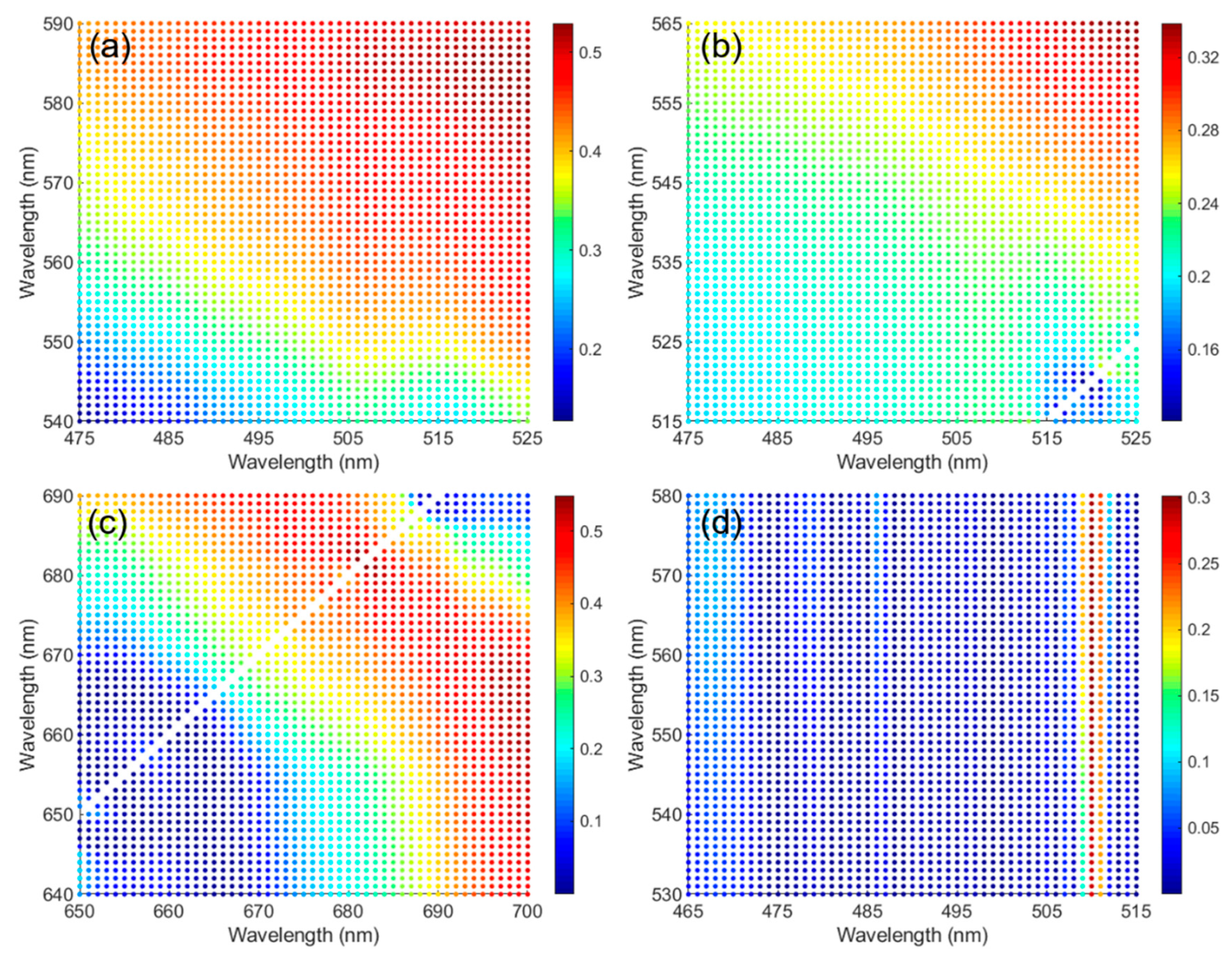
4.2.1. Optimization of Red Tide Indexes

Optimization of the four red tide indexes was conducted via wavelength band adjustment. The wavelength band was changed at intervals of 1 nm around the wavelength band originally used for each red tide index, and adjustments were performed within a range that did not exceed each intrinsic wavelength band. Optimization was performed until the R² values converged for a specific wavelength band, and among the results, the wavelength that showed the strongest correlation with M. polykrikoides cell abundance was selected for index optimization. Figure 4 shows the optimization results for the FRTD index, the SS index, the KBBI, and the MRI. Dot colors represent R² values between the red tide indexes and measured M. polykrikoides cell abundances. The FRTD index values which were calculated using the original wavelength band showed a correlation of 0.35 with cell abundance (Figure 4a). The maximum R² (0.53) of the optimized FRTD index was obtained when 490 nm was shifted to 524 nm and 555 nm to 583 nm. In the optimized SS index, the blue band of 443 nm was not altered, while the two green bands were shifted (Figure 4b). The SS index that used wavelengths of 490 and 510 nm had an R² of 0.2 and the highest R² (0.33) was obtained using 520 and 560 nm. The KBBI originally used wavelength bands of 667 and 678 nm and had an R² of 0.36 (Figure 4c). The optimized KBBI showed the highest R² (0.54) at wavelengths of 666 and 698 nm. Similar to the SS index, the original MRI shifted to 490 and 555 nm without changing the blue band at 443 nm. Unlike the other indexes, the R² values of the MRI were distributed in a straight line (Figure 4d). The original MRI had the lowest R² (0.014) among the four red tide indexes investigated. The highest R² (0.30) for MRI was observed using wavelengths of 510 and 566 nm. The wavelength bands with the highest R² for each index were selected to optimize the red tide indexes for quantification of red tide cell abundance.

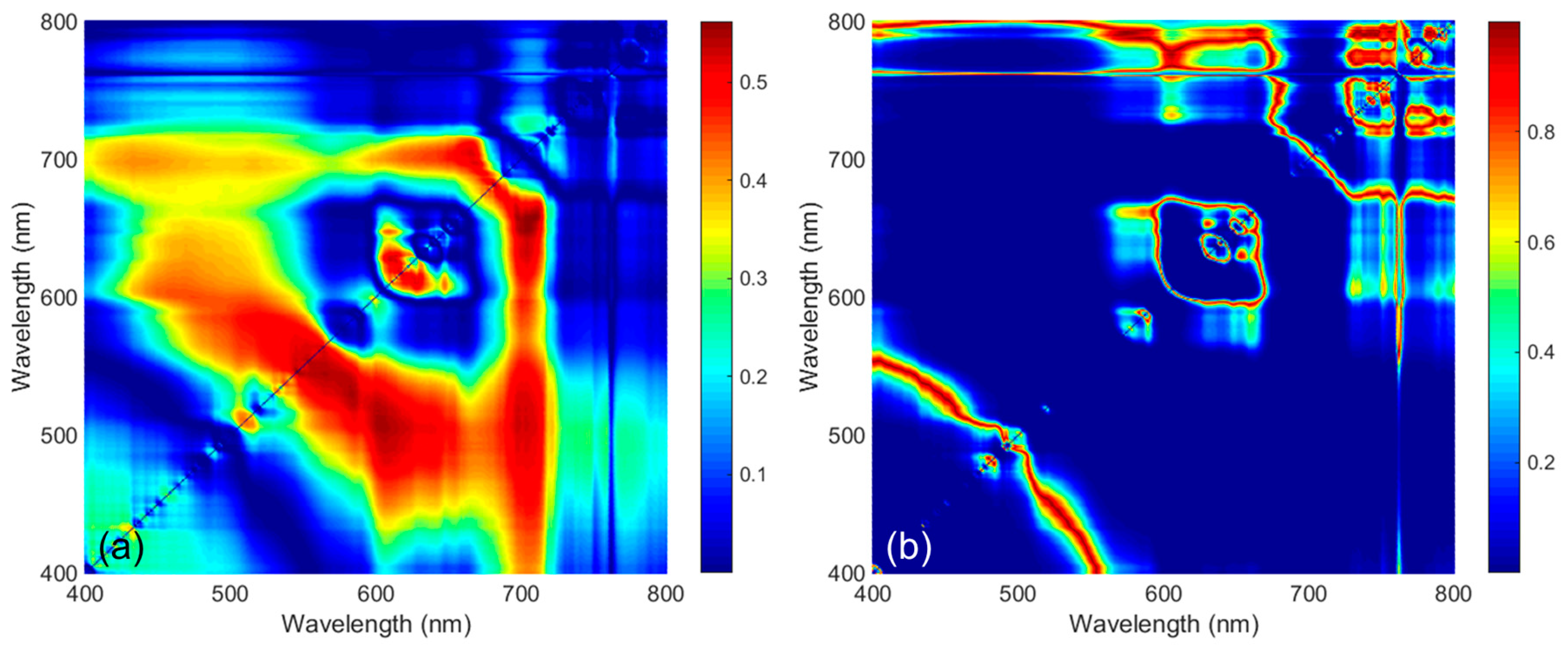
4.2.2. Band Correlation Analyses

To investigate the relationship between M. polykrikoides cell abundance and in situ spectra, 49 pairs were used for correlation analyses. On the basis of a threshold cell abundance of 1000 cells mL⁻¹, we divided the data into two subgroups of <1000 cells mL⁻¹ and >1000 cells mL⁻¹. Figure 5 shows the R² values between M. polykrikoides cell abundance and in situ R_rs spectra at each wavelength band. For the total range group with 49 pairs, it showed the highest correlation (R² = 0.21) with M. polykrikoides cell abundance in the wavelength of 503 nm among the entire wavelength range. The subgroups of >1000 cells mL⁻¹ and <1000 cells mL⁻¹ showed the strongest correlations with M. polykrikoides cell abundance at 562 nm (R² = 0.23) and 503 nm (R² = 0.12), respectively. The subgroup of <1000 cells mL⁻¹ varied more than the subgroup of >1000 cells mL⁻¹, as evidenced by its lower R² value, and showed the strongest correlation among the three groups. In addition, the green wavelength band showed a strong correlation at high M. polykrikoides cell abundance.

Figure 6 shows the R² and p-values of the in situ R_rs spectral ratio for each wavelength band. R² represents the relationship between M. polykrikoides cell abundance and in situ R_rs at the wavelength shown on the x-axis divided by that on the y-axis, and it shows a symmetrical distribution. In addition, ratios around 700 nm showed the highest R² values. The distribution of p-values showed the same symmetrical structure as R² values. In the range with high R² values, low p-values were observed. The maximum value of R² was 0.56 at 704/649 nm, and the corresponding valid p-value was 6.07 × 10⁻¹⁰. The R² of the band ratio index was 2.68 times greater than that of the single-band index (R² = 0.21).

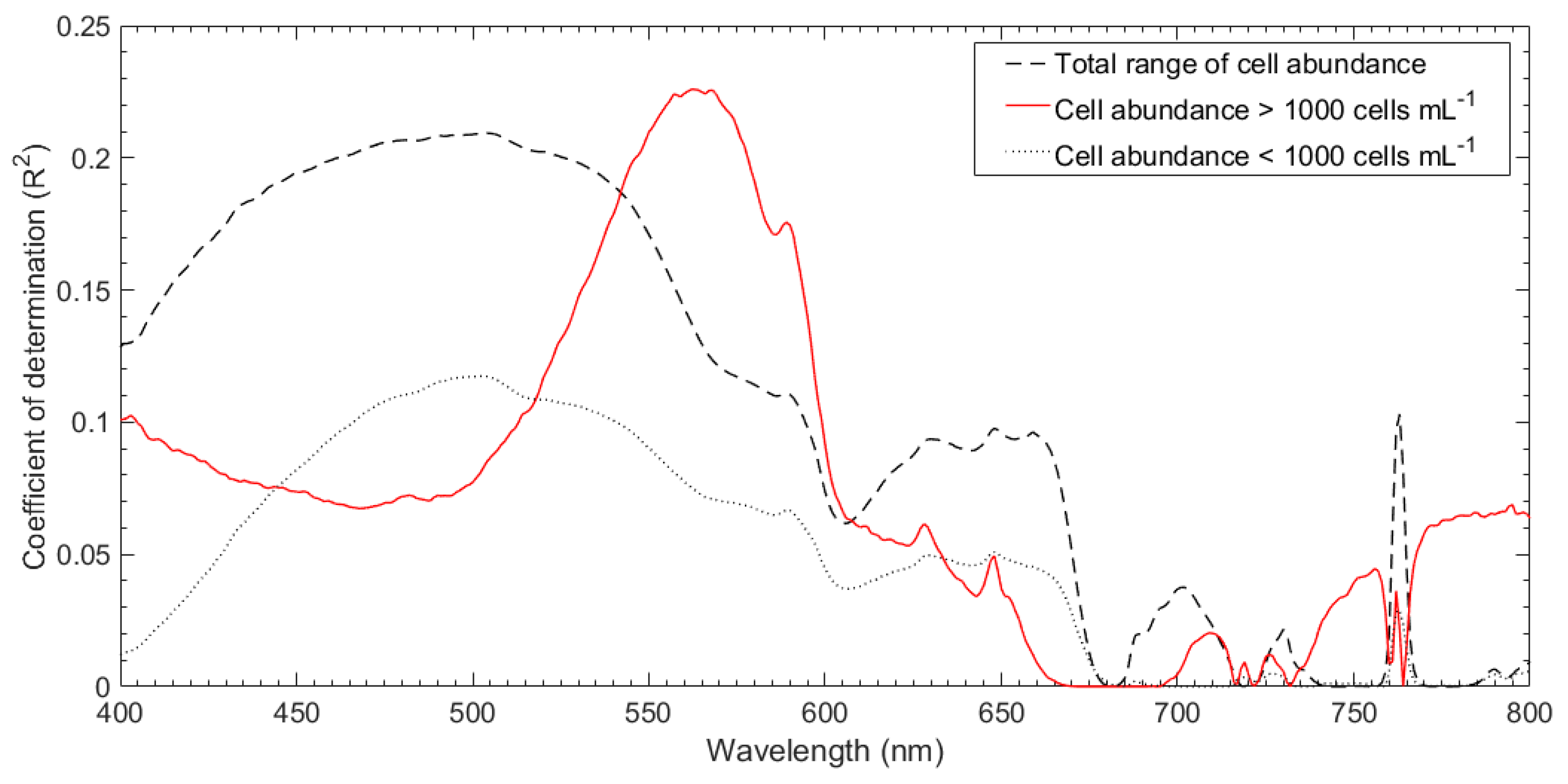
4.2.3. Green-to-Fluorescence Ratio (GFR) Index

Figure 7 shows the average spectra of in situ R_rs with a range of M. polykrikoides cell abundances. The black dotted line represents cell abundances of 100 cells mL⁻¹ or less. The black dashed and red lines indicate M. polykrikoides cell abundances of 100 and 1000 cells mL⁻¹ or higher, respectively. Each spectrum was calculated as the average of the spectra at all sampling points for each range. A comparison with spectra representing cell abundances below 1000 cells mL⁻¹, showed that the spectra for more than 1000 cells mL⁻¹ displayed sharper peaks near 570 and 690 nm. The slope of the peak point around 570 nm became steeper as the peak intensity near 690 nm strengthened, due to the combined effects of increased pigment absorption and fluorescence emissions near 660–700 nm, strong water absorption above 700 nm, and backscattering of red and near infrared wavelengths by biological particles [55]. The spectrum for abundances greater than 1000 cells mL⁻¹ shows distinct triangular peaks in the green and red wavelengths, and this spectral pattern is typical of M. polykrikoides blooms. For the spectra representing cell abundances of 100 cells mL⁻¹ or more and 1000 cells mL⁻¹ or less, the spectral shapes of the peak points were relatively smooth as compared with those representing 1000 cells mL⁻¹ or more.

The main purpose of the new red tide indexes is to exploit red tide spectral characteristics in the green and red wavelengths. In situ R_rs measurements along the south coast of Korea showed that the spectra above 1000 cells mL⁻¹ displayed sharper peaks near 570 and 690 nm as compared with spectra below 1000 cells mL⁻¹ of cell abundance (Figure 7). In addition, as M. polykrikoides cell abundance increased, the slope at the peak point gradually increased. Considering these characteristics, the proposed index defines the green-to-fluorescence ratio (GFR) index as:

$$\mathrm{GFR}=\frac{R_{rs}\left({\lambda }_{Green}^{+}\right)}{R_{rs}\left({\lambda }_{Green}^{-}\right)}\ast \frac{R_{rs}\left({\lambda }_{Flou}^{+}\right)}{R_{rs}\left({\lambda }_{Flou}^{-}\right)}$$

(7)

where ${\lambda }_{Red}^{+}$ is the central band (583 nm), ${\lambda }_{Red}^{-}$ is the next lower band (524 nm), ${\lambda }_{Flou}^{-}$ is the next higher band (666 nm), and ${\lambda }_{Flou}^{+}$ is the higher band (698 nm). Among the wavelengths used in the GFR index, 524 and 583 nm are the green wavelength bands used in the optimized FRTD index and 666 and 698 nm are the fluorescence wavelength bands used in the optimized KBBI.

4.2.4. Evaluation of the New Red Tide Index for Quantifying Red Tide Cell Abundance

The calculated red tide index values for the measured R_rs spectra were converted into red tide cell abundances through first-order polynomial fitting. The optimization results for the red tide indexes showed significant improvement as compared with the original indexes. The optimized FRTD index had the highest R² value (0.55), and the R² of the optimized MRI (0.30) increased 21.8 times as compared with that of the original MRI (R² = 0.01). For all indexes, the RMSE and MBE between the estimated cell abundance and measured cell abundance were reduced by 13% and 22%, respectively. The R² of the band ratio index (0.56) increased 2.68 times as compared with that of the single band index (0.21). The GFR index had a moderate correlation, with R² of 0.45, RMSE of 880.95 cells mL⁻¹, and MBE of −0.20 cells mL⁻¹. To analyze the precision of the indexes, we divided cell abundance data into the following three subgroups based on thresholds of 100 and 1000 cells mL⁻¹: high (HC, >1000 cells mL⁻¹), moderate (MC, 100 cells mL⁻¹ < cell abundance < 1000 cells mL⁻¹), and low (LC, <100 cells mL⁻¹), respectively. For each subgroup, the RMSE and MBE values were calculated. All subgroups of optimized indexes had reduced RMSE and MBE values as compared with the original indexes. In the LC group, the mean RMSE and MBE values in the optimized indexes were 613.87 and 483.58 cells mL⁻, respectively, representing decreases of 11% and 17%, respectively, as compared with the original indexes. The GFR index in the LC group had RMSE and MBE values of 576.77 and 529.97 cells mL⁻¹, respectively. The RMSE and MBE values of the LC group indicated significant error in estimation of red tide cell abundances of 100 cells mL⁻¹ or less.

To reduce error, a process of finding the best-fit model between the calculated index value and the measured M. polykrikoides cell abundance was employed. The performance of red tide indexes was good when the second-order polynomial and power regression models were applied.

Table 4. Performance of one proposed and four published red tide indexes. TC indicates the total cell abundance group (all samples). HC (high cell abundance), MC (middle cell abundance), and LC (low cell abundance) represent cell abundance >1000 cells mL⁻¹, 100 < cell abundance < 1000 cells mL⁻¹, and cell abundance <100 cells mL⁻¹, respectively.

Red Tide Index	R2	RMSE				MBE
		TC	LC	MC	HC	TC	LC	MC	HC
FRTD index	0.26	1084.92	140.32	861.86	1857.60	−376.77	47.98	−33.16	−1369.08
Optimized FRTD index	0.38	1047.25	72.60	484.04	1905.02	−302.75	37.88	−292.00	−871.55
SS index	0.08	1420.12	87.21	433.87	2623.88	−354.80	53.28	−182.88	−1172.57
Optimized SS index	0.47	858.53	265.56	723.23	1419.70	−169.17	154.97	184.53	−1004.87
KBBI	0.09	1252.09	80.34	1150.55	2083.69	−444.98	43.69	131.76	−1742.14
Optimized KBBI	0.41	941.00	95.08	626.38	1657.72	−294.64	40.89	−91.36	−1020.09
MRI	0.00019	1405.10	108.77	844.05	2505.99	−668.00	107.87	−151.34	−2385.47
Optimized MRI	0.05	1413.95	112.78	505.56	2599.50	−536.19	112.12	−465.40	−1661.97
Single band index	0.24	1278.70	184.64	454.37	2343.03	−672.55	119.84	−390.22	−2216.34
Band ratio index	0.41	1028.92	62.79	631.88	1832.11	−282.07	36.10	−133.57	−932.05
GFR index	0.42	966.04	90.86	487.90	1746.06	−306.92	43.29	−251.16	−930.05

Units of root mean square error (RMSE) and mean bias error (MBE) are cells mL⁻¹.

shows the correlations between estimated and measured cell abundance. Cell abundance was calculated using the formula generated from the relationship between each index and the measured cell abundance. To evaluate the performance of the red tide indexes, R², RMSE, and MBE values were calculated for each red tide index. The RMSE and MBE values were also calculated for each subgroup (HC, MC, and LC). The optimized red tide indexes showed higher R², and lower RMSE and MBE values than the original indexes, and the band ratio index showed the same results as the single band index. The three optimized indexes, aside from MRI, the band ratio index, and the GFR index, all showed similar correlations. The optimized SS index had the highest R² (0.47), along with the lowest RMSE value (858.53 cells mL⁻¹) and MBE value (−169.17 cells mL⁻¹) among published red tide indexes. The GFR index showed a strong correlation, with an R² of 0.42, a RMSE value of 966.04 cells mL⁻¹, and an MBE value of −306.92 cells mL⁻¹. After dividing the dataset into subgroups, red tide index optimization generally led to decreases in the RMSE and MBE values, although these values tended to increase for some groups. For example, the RMSE value showed a significant decrease in the HC group, but increased in the MC and LC groups. The band ratio index for the LC group had the smallest RMSE value (62.79 cells mL⁻¹) and MBE value (36.10 cells mL⁻¹). The GFR index for the LC group had an RMSE value of 90.86 cells mL⁻¹ and an MBE value of 43.29 cells mL⁻¹. In addition, the GFR index showed good results for RMSE and MBE in the HC and MC groups.

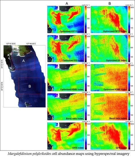
4.3. Performance of New Indexes Using Hyperspectral Imagery

To generate a distribution map of M. polykrikoides cell abundance, the formulas generated from the relationship between each index and measured cell abundance data were applied to each pixel of HSI acquired along the coast of Yeosu on 8 August 2018. The difference between wavelength bands used in the index and HSI did not exceed 1 nm. For example, for the optimized FRTD index using 524 and 583 nm, the wavelength bands of 523.69 and 583.67 nm were used. In the corresponding daily red tide report provided by the NIFS, the M. polykrikoides bloom was reported to have a cell abundance of less than 1000 cells mL⁻¹ along the coast near Bangjukpo Beach in Yeosu. In addition, this report noted that red tide organisms were present at a cell abundance of 100 cells mL⁻¹ or less where ocean color was normal outside of red tide patches. However, during the actual field survey, we found a wide range of cell abundances and a high density of red tide patches near Bangjukpo Beach in Yeosu. The reddish M. polykrikoides patches were clearly observed in the true-color composite image obtained from HSI as compared with the surrounding seawater (Figure 8). Some patches were distributed among aquaculture farm structures. Figure 8 shows M. polykrikoides cell abundance maps generated by applying the optimized red tide indexes, aside from the MRI, band ratio index, and GFR index. The red tide cell abundance maps were created using the range and distribution from cell abundance estimation. The cell abundance map created using the optimized KBBI and band ratio index did not show the pattern of red tide patches observed in the true-color composite image. However, patches were clearly distinguished from the surrounding seawater on the cell abundance maps based on the optimized FRTD index, the optimized SS index, and the GFR index. In particular, the lower portion of the SS index image showed a clearer red tide patch than the other index images. In terms of cell abundance estimation, all indexes, except the optimized SS and KBBI indexes, could estimate cell abundance ranges below 100 cells mL⁻¹ and near 5000 cells mL⁻¹. In the areas corresponding to Sections A and B in Figure 8, cell abundances of up to 4647.13 cells mL⁻¹ were obtained at the time of the field survey. This indicates that the cell range of abundance estimates obtained using the red tide indexes is quite appropriate. However, the optimized SS and KBBI indexes only estimated cell abundances of up to 2000 and 3000 cells mL⁻¹, respectively.

The comparison of the five red tide indexes was performed using 14 matchups between the measured M. polykrikoides cell abundances and the cell abundances calculated from HSI R_rs (Figure 9). For the LC group, which had low cell abundances (<100 cells mL⁻¹), all red tide indexes showed relatively good results. However, for the MC group (>100 and <1000 cells mL⁻), a large variation in cell abundance was estimated for all indexes. In addition, for the HC group (>1000 cells mL⁻¹), an underestimation was observed in all indexes except the GFR index.

Table 5. Performance of red tide indexes applied to atmospherically corrected HSI R_rs.

Red Tide Index	R2	RMSE (cells mL−1)				MBE (cells mL−1)
		TC	LC	MC	HC	TC	LC	MC	HC
Optimized FRTD index	0.39	1485.06	1.24	486.88	2544.40	−863.95	0.35	−466.42	−2312.48
Optimized SS index	0.40	1130.46	2.09	629.12	1896.39	−494.40	−1.38	72.15	−1524.56
Optimized KBBI index	0.40	1101.82	1.73	646.00	1841.64	−420.12	−0.32	426.01	−1515.52
Band Ratio index	0.36	1366.58	1.56	311.71	2354.63	−741.86	−0.16	−165.31	−2126.19
GFR index	0.52	877.98	1.72	1200.75	1203.11	−18.42	0.94	817.66	−547.17

TC indicates the total cell abundance group (all samples). HC (high cell abundance), MC (middle cell abundance), and LC (low cell abundance) represent cell abundance >1000 cells mL⁻¹, 100 < cell abundance < 1000 cells mL⁻¹, and cell abundance <100 cells mL⁻¹, respectively.

shows the performance of each red tide index. The R² between the measured M. polykrikoides cell abundance and red tide indexes ranged from 0.36 (band ratio index) to 0.52 (GFR index). For the LC group, the RMSE and MBE values of all indexes were similar for all indexes. For the MC group, the RMSE and MBE values were the smallest for the band ratio index and optimized SS index, respectively. For the HC group, the GFR index had the lowest RMSE and MBE values. Overall, the GFR index showed the best performance, with high accuracy when applied to atmospherically corrected HSI.

5. Discussion

5.1. Uncertainty of Spectral Measurement

The spectral data used in this study were obtained through a total of six field surveys and was accompanied by various uncertainties. The measured spectral values could vary depending on the type of equipment used for measurement, the method of measurement, and the seawater environmental conditions at the time of measurement. Spectra were measured during the field surveys for this study using Fieldspec3 (serial numbers 16031 and 16395), Fieldspec4 (serial number 18701), and Profiler II instruments. To determine the effect on spectrum of the measurement instrument, a comparison among spectra measured using these three instruments at station R02 (34°34.973′ N, 127°40.873′ E) was performed. All acquired spectra were converted into R_rs. The two spectra obtained using the Fieldspec3 instruments with different serial numbers followed a similar pattern and had a high correlation (R² = 0.96). Spectra measured using the Profiler II showed a pattern similar to that obtained from the Fieldspec devices. However, the spectral values were relatively high at wavelengths below 600 nm and relatively low at wavelengths above 600 nm. The correlations of Profiler II and Fieldspec spectra were weaker than those between Fieldspec devices (R² = 0.53), but the shapes of Profiler II and Fieldspec spectra were very similar. This difference could be due to the different measurement methods used by the instruments. Fieldspec measured spectra above the sea surface from the ship, whereas Profiler II used spectra measured 1 m below the sea surface. Although this study used a variety of instruments to obtain a large amount of data, there was no discrepancy among data sources. In addition to the differences among instruments, errors in the measured spectra could also be caused by environmental conditions at the time of the measurements. Indeed, spectra measured at the same location almost simultaneously showed similar patterns, but their overall values were biased. This is probably due to the amount of light, which changes instantaneously in E_d measurements, combined with errors in the measurement methods used for L_sky and L_t. To reduce such errors, we conducted bias correction through an offset adjustment of the acquired spectra to maintain uniform results [48].

5.2. Uncertainty of Atmospheric Correction

The performance of atmospheric correction depends on the observation target and atmospheric conditions. In this study, atmospheric correction and verification were performed for seawater only. The signal detected from sea surface was very weak, which made obtaining accurate seawater signals through atmospheric correction difficult as compared with land surfaces. Because atmospheric radiance caused by molecular and aerosol scattering could account for more than 90% of total radiance, atmospheric correction had a large impact on the results [56]. Under these conditions, an accurate estimation of atmospherically corrected R_rs is essential for detection of colored water constituents such as red tide species and other phytoplankton, as these constituents absorb light and weaken the reflected signal. On the one hand, our atmospheric correction results indicate that the QUAC method alone shows poor performance for seawater. On the other hand, based on analyses of the correlation between atmospherically corrected HSI R_rs and in situ R_rs for a fluorescent dye with a stronger signal than seawater, atmospheric correction using only the QUAC method showed a moderate correlation (R² = 0.50). In particular, the correlation was very strong in the 500–700 nm wavelength region (R² = 0.94). In situ and atmospherically corrected HSI R_rs spectra showed very similar shapes up to 590 nm, which was near the maximum, with a mean value of 0.028 sr⁻¹. This value is about three times greater than 0.01 sr⁻¹, the maximum value of the red tide spectrum. However, both the red tide and fluorescent dye spectra showed weak correlations and did not approach zero in the wavelength range above 700 nm. This phenomenon has been observed in other studies. Mobley et al. [48] found that airborne HSI spectra did not approach zero for wavelengths beyond 700 nm, similar to our results. Dierssen et al. [57] concluded that HSI spectral values were too high in the red wavelengths, and Kohler [58] found that both an offset and gain adjustment were necessary to bring HSI spectra into agreement with ground-truth R_rs spectra. Louchard et al. [59] adjusted the spectra from HSI spectra by subtracting the difference between the HSI and in situ spectra. These findings suggest that the QUAC method is effective for seawater targets with strong signals in the wavelength range below 700 nm.

Atmospheric conditions also have a significant impact on atmospheric correction results. If the atmosphere is not clear, i.e., if the degree of cloud or haze is high when the HSI is acquired, the results of atmospheric correction can be significantly affected. At the time of the field survey when HSI was acquired on 8 August 2018, the atmosphere was hazy, while the HSI field survey on 26 September 2019 occurred under a clear atmosphere. This difference affected the atmospheric correction results for HSI. In 2019, a strong correlation (R² = 0.85) was obtained between R_rs corrected using the QUAC method combined with the EL method and in situ R_rs, whereas, in 2018, that correlation was weaker (R² = 0.56). In addition to atmospheric conditions, the following factors can affect the performance of atmospheric correction. The difference in acquisition time between in situ spectra and HSI can cause a spectral difference. Because airborne monitoring and the field survey conducted in this study differed by up to 4 h, this impact cannot be ignored. In addition, in situ spectra were acquired through discrete sampling, whereas the corresponding HSI R_rs were obtained with a spatial resolution of 2 m. Red tide patches varied considerably within a few meters, so this difference in spectral acquisition methods could result in poorer atmospheric correction performance.

5.3. Performance of New Red Tide Index

In this study, pairs of M. polykrikoides cell abundances and in situ R_rs spectra were used to explore new indexes for quantitative analyses of red tides. After applying the proposed new indexes to atmospherically corrected HSI R_rs, the GFR index showed the best performance among new indexes, with the highest accuracy paired with low RMSE and MBE values. Several factors can affect the performance of the new indexes. First, incompleteness of the proposed new index caused by the limited number and diversity of data pairs can affect its performance. Among a total of 49 pairs, 14 pairs had cell abundances greater than 1000 cells mL⁻¹ and only one pair was above 4000 cells mL⁻¹. In addition, 12 pairs fell between 100 cells mL⁻¹ and 1000 cells mL⁻¹ but only two of those pairs were between 100 cells mL⁻¹ and 500 cells mL⁻¹. This deficiency can strongly affect the regression model used for estimating cell abundance, which makes it difficult to estimate cell abundance beyond the scope of the data. Second, factors related to matching of the red tide cell abundance estimated using HSI with the measured cell abundance can affect performance. Imperfections in the atmospheric correction of HSI used for verification are a major factor in reducing performance. Furthermore, in situ cell abundance data obtained through discrete sampling inevitably differs from cell abundance data estimated from HSI with a spatial resolution of 2 m. In addition, the spatial distribution of red tide patches can affect verification accuracy. Red tide patches vary significantly within a few meters and tend to move with ocean currents or winds. Shin et al. [29] confirmed that red tide patches moved slightly northward between two satellite images obtained within 1 h. Thus, the difference between the sampling time used to estimate in situ cell abundances and HSI acquisition time can reduce verification accuracy. In particular, because M. polykrikoides is characterized by vertical migration, the difference in sampling time can be an important factor affecting performance. Park et al. [60] reported that M. polykrikoides moved toward the sea surface beginning at approximately 8:00 (GMT +09) in the morning and the surface cell abundance peaked around 16:00 (GMT +09), decreasing thereafter. Choi et al. [26] found that the M. polykrikoides cell abundance was highest at 14:30 (GMT +09) when investigating hourly variation. Noh et al. [27] found that red tide intensity increased around midday, with gradual expansion of high-concentration patches from 10:30 to 14:30 (GMT +09). In this study, the HSI, which showed clear red tide patches, was acquired at about 17:18 (GMT +09) on 8 August 2018; according to previous research, red tide intensity was decreasing at that time. During the field survey, water sampling differed by up to 4 h from the HSI acquisition time, which could affect the accuracy of verification.

6. Conclusions

In this study, we proposed new indexes for quantifying M. polykrikoides cell abundance using HSI. The atmospheric correction of HSI was conducted using the QUAC method and the EL method. After optimization of the published red tide indexes and band correlation analyses, the GFR index was proposed as a new red tide index for quantifying M. polykrikoides cell abundance. The performance of the new index was evaluated using HSI, and a cell abundance map of M. polykrikoides was generated. The major results are as follows:

• Atmospheric correction was performed using the QUAC method combined with the EL method, and the results showed good performance (R² = 0.87). The higher the wavelength band, the lower the performance. In addition, the performance during the period when the red tide bloom did not occur was higher than the performance at the time when the red tide occurred.
• As a result of optimizing published red tide indexes, the accuracy of all indexes was improved as compared with the original indexes. The band ratio index showed better performance than the single band index. Considering the spectral characteristics of red tide species, the new GFR index was proposed. The optimized FRTD index, band ratio index, and GFR index were capable of estimating high cell abundances, up to 5000 cells mL⁻¹. In addition, the red tide patch was most pronounced in the M. polykrikoides cell abundance maps based on the optimized FRTD index, optimized SS index, and GFR index. Among these indexes, the GFR index showed the best performance, as verified using HSI R_rs. In addition, it showed the lowest RMSE and MBE values in the total group, especially the HC group.

Our newly proposed GFR index was developed and validated for optically complex waters along the south coast of Korea. The red tide cell abundance map generated using the GFR index allowed us to determine the precise spatial distribution of a M. polykrikoides bloom and cell abundance estimation with reasonably high accuracy. This method provides a basis for establishing countermeasures to reduce damage caused by M. polykrikoides blooms.

References

1. Jeong, H.J.; Kang, C.K. Understanding and managing red tides in Korea Preface. Harmful Algae 2013, 30, S1–S2. [Google Scholar] [CrossRef]
2. Lee, C.K.; Park, T.G.; Park, Y.T.; Lim, W.A. Monitoring and trends in harmful algal blooms and red tides in Korean coastal waters, with emphasis on Cochlodinium polykrikoides. Harmful Algae 2013, 30, S3–S14. [Google Scholar] [CrossRef]
3. Gobler, C.; Gobler, C.J.; Anderson, O.R.; Berry, D.L.; Burson, A.; Koch, F.; Rodgers, B.; Koza-Moore, L.; Goleski, J.; Allam, B.; et al. Characterization, dynamics, and ecological impacts of harmful Cochlodinium polykrikoides blooms on eastern Long Island, NY, USA. Harmful Algae 2008, 7, 293–307. [Google Scholar] [CrossRef]
4. Park, T.G.; Lim, W.A.; Park, Y.T.; Lee, C.K.; Jeong, H.J. Economic impact, management and mitigation of red tides in Korea. Harmful Algae 2013, 30 (Suppl. 1), S131–S143. [Google Scholar] [CrossRef]
5. Tang, Y.Z.; Gobler, C.J. Characterization of the toxicity of Cochlodinium polykrikoides isolates from Northeast US estuaries to finfish and shellfish. Harmful Algae 2009, 8, 454–464. [Google Scholar] [CrossRef]
6. Whyte, J.N.C.; Haigh, N.; Ginther, N.G.; Keddy, L.J. First record of blooms of Cochlodinium sp. (Gymnodiniales, Dinophyceae) causing mortality to aquacultured salmon on the west coast of Canada. Phycologia 2001, 40, 298–304. [Google Scholar] [CrossRef]
7. Forecast ∙ Breaking News of the National Institute of Fisheries Science (NIFS). Available online: www.nifs.go.kr\redtideInfo (accessed on 27 May 2020).
8. National Institute of Fisheries Science (NIFS). Harmful Algal Blooms in Korean Coastal Waters; National Institute of Fisheries Science: Busan, Korea, 2015. [Google Scholar]
9. Carder, K.L.; Chen, F.R.; Lee, Z.P.; Hawes, S.K.; Kamykowski, D. Semianalytic Moderate-Resolution Imaging Spectrometer algorithms for chlorophyll and absorption with bio-optical domains based on nitrate-depletion temperatures. J. Geophys. Res. Oceans 1999, 104, 5403–5421. [Google Scholar] [CrossRef]
10. Cannizzaro, J.P.; Carder, K.L.; Chen, F.R.; Heil, C.A.; Vargo, G.A. A novel technique for detection of the toxic dinoflagellate, Karenia brevis, in the Gulf of Mexico from remotely sensed ocean color data. Cont. Shelf Res. 2008, 28, 137–158. [Google Scholar] [CrossRef]
11. Morel, A. Optical modeling of the upper ocean in relation to its biogenous matter content (case I waters). J. Geophys. Res. Oceans 1988, 93, 10749–10768. [Google Scholar] [CrossRef] [Green Version]
12. Suh, Y.S.; Jang, L.H.; Lee, N.K.; Ishizaka, J. Feasibility of red tide detection around Korean waters using satellite remote sensing. Fish. Aqua. Sci. 2004, 7, 148–162. [Google Scholar] [CrossRef] [Green Version]
13. Tomlinson, M.C.; Wynne, T.T.; Stumpf, R.P. An evaluation of remote sensing techniques for enhanced detection of the toxic dinoflagellate, Karenia brevis. Remote Sens. Environ. 2009, 113, 598–609. [Google Scholar] [CrossRef]
14. Amin, R.; Zhou, J.; Gilerson, A.; Gross, B.; Moshary, F.; Ahmed, S. Novel optical techniques for detecting and classifying toxic dinoflagellate Karenia brevis blooms using satellite imagery. Opt. Express 2009, 17, 9126–9144. [Google Scholar] [CrossRef] [PubMed]
15. Lou, X.; Hu, C. Diurnal changes of a harmful algal bloom in the East China Sea: Observations from GOCI. Remote Sens. Environ. 2014, 140, 562–572. [Google Scholar] [CrossRef]
16. Ahn, Y.H.; Shanmugam, P. Detecting the red tide algal blooms from satellite ocean color observations in optically complex Northeast-Asia Coastal waters. Remote Sens. Environ. 2006, 103, 419–437. [Google Scholar] [CrossRef]
17. Ghanea, M.; Moradi, M.; Kabiri, K. A novel method for characterizing harmful algal blooms in the Persian Gulf using MODIS measurements. Adv. Space Res. 2016, 58, 1348–1361. [Google Scholar] [CrossRef]
18. Hu, C.; Muller-Karger, F.E.; Taylor, C.J.; Carder, K.L.; Kelble, C.; Johns, E.; Heil, C.A. Red tide detection and tracing using MODIS fluorescence data: A regional example in SW Florida coastal waters. Remote Sens. Environ. 2005, 97, 311–321. [Google Scholar] [CrossRef]
19. Kim, Y.; Byun, Y.; Kim, Y.; Eo, Y. Detection of Cochlodinium polykrikoides red tide based on two-stage filtering using MODIS data. Desalination 2009, 249, 1171–1179. [Google Scholar] [CrossRef]
20. Shin, J.S.; Min, J.E.; Ryu, J.H. A study on red tide surveillance system around the Korean coastal waters using GOCI. Korean J. Remote Sens. 2017, 33, 213–230. [Google Scholar]
21. Son, Y.B.; Kang, Y.H.; Ryu, J.H.; Jeong, J.C. Satellite detection of harmful algal bloom occurrences in Korean waters. Korean J. Remote Sens. 2012, 28, 531–548. [Google Scholar] [CrossRef]
22. Stumpf, R.P.; Culver, M.E.; Tester, P.A.; Tomlinson, M.; Kirkpatrick, G.J.; Pederson, B.A.; Truby, E.; Ransibrahmanakul, V.; Soracco, M. Monitoring Karenia brevis blooms in the Gulf of Mexico using satellite ocean color imagery and other data. Harmful Algae 2003, 2, 147–160. [Google Scholar] [CrossRef]
23. Tao, B.; Mao, Z.; Lei, H.; Pan, D.; Shen, Y.; Bai, Y.; Zhu, Q.; Li, Z. A novel method for discriminating Prorocentrum donghaiense from diatom blooms in the East China Sea using MODIS measurements. Remote Sens. Environ. 2015, 158, 267–280. [Google Scholar] [CrossRef]
24. Tester, P.A.; Stumpf, R.P.; Steidinger, K.A. Ocean color imagery: What is the minimum detection level for Gymnodinium breve blooms. Harmful Algae 1998, 149–151. [Google Scholar]
25. Tomlinson, M.C.; Stumpf, R.P.; Ransibrahmanakul, V.; Truby, E.W.; Kirkpatrick, G.J.; Pederson, B.A.; Gabriel, A.V.; Heil, C.A. Evaluation of the use of SeaWiFS imagery for detecting Karenia brevis harmful algal blooms in the eastern Gulf of Mexico. Remote Sens. Environ. 2004, 91, 293–303. [Google Scholar] [CrossRef]
26. Choi, J.K.; Min, J.E.; Noh, J.H.; Han, T.H.; Yoon, S.; Park, Y.J.; Moon, J.E.; Ahn, J.H.; Ahn, S.M.; Park, J.H. Harmful algal bloom (HAB) in the East Sea identified by the Geostationary Ocean Color Imager (GOCI). Harmful Algae 2014, 39, 295–302. [Google Scholar] [CrossRef]
27. Noh, J.H.; Kim, W.; Son, S.H.; Ahn, J.H.; Park, Y.J. Remote quantification of Cochlodinium polykrikoides blooms occurring in the East Sea using geostationary ocean color imager (GOCI). Harmful Algae 2018, 73, 129–137. [Google Scholar] [CrossRef]
28. Tomas, C.R.; Smayda, T.J. Red tide blooms of Cochlodinium polykrikoides in a coastal cove. Harmful Algae 2008, 7, 308–317. [Google Scholar] [CrossRef]
29. Shin, J.; Kim, K.; Son, Y.B.; Ryu, J.H. Synergistic effect of multi-sensor Data on the detection of Margalefidinium polykrikoides in the South Sea of Korea. Remote Sens. 2019, 11, 36. [Google Scholar] [CrossRef] [Green Version]
30. Kim, W.; Moon, J.E.; Park, Y.J.; Ishizaka, J. Evaluation of chlorophyll retrievals from Geostationary Ocean Color Imager (GOCI) for the North-East Asian region. Remote Sens. Environ. 2016, 184, 482–495. [Google Scholar] [CrossRef]
31. O’Reilly, J.E.; Maritorena, S.; Mitchell, B.G.; Siegel, D.A.; Carder, K.L.; Garver, S.A.; Kahru, M.; McClain, C. Ocean color chlorophyll algorithms for SeaWiFS. J. Geophys. Res. Oceans 1998, 103, 24937–24953. [Google Scholar] [CrossRef] [Green Version]
32. Soto, I.M.; Cannizzaro, J.; Muller-Karger, F.E.; Hu, C.; Wolny, J.; Goldgof, D. Evaluation and optimization of remote sensing techniques for detection of Karenia brevis blooms on the West Florida Shelf. Remote Sens. Environ. 2015, 170, 239–254. [Google Scholar] [CrossRef]
33. Awad, M. Sea water chlorophyll-a estimation using hyperspectral images and supervised artificial neural network. Ecol. Inf. 2014, 24, 60–68. [Google Scholar] [CrossRef]
34. Duan, H.; Ma, R.; Hu, C. Evaluation of remote sensing algorithms for cyanobacterial pigment retrievals during spring bloom formation in several lakes of East China. Remote Sens. Environ. 2012, 126, 126–135. [Google Scholar] [CrossRef]
35. Jeon, E.I.; Kang, S.J.; Lee, K.Y. Estimation of chlorophyll-a concentration with semi-analytical algorithms using airborne hyperspectral imagery in Nakdong river of South Korea. Spat. Inf. Res. 2019, 27, 97–107. [Google Scholar] [CrossRef]
36. Kudela, R.M.; Palacios, S.L.; Austerberry, D.C.; Accorsi, E.K.; Guild, L.S.; Torres-Perez, J. Application of hyperspectral remote sensing to cyanobacterial blooms in inland waters. Remote Sens. Environ. 2015, 167, 196–205. [Google Scholar] [CrossRef] [Green Version]
37. Li, L.; Sengpiel, R.E.; Pascual, D.L.; Tedesco, L.P.; Wilson, J.S.; Soyeux, E. Using hyperspectral remote sensing to estimate chlorophyll-a and phycocyanin in a mesotrophic reservoir. Int. J. Remote Sens. 2010, 31, 4147–4162. [Google Scholar] [CrossRef]
38. Sawtell, R.W.; Anderson, R.; Tokars, R.; Lekki, J.D.; Shuchman, R.A.; Bosse, K.R.; Sayers, M.J. Real time HABs mapping using NASA Glenn hyperspectral imager. J. Great Lakes Res. 2019, 45, 596–608. [Google Scholar] [CrossRef]
39. Sengpiel, R.E. Using Airborne Hyperspectral Imagery to Estimate Chlorophyll a and Phycocyanin in Three Central Indiana Mesotrophic to Eutrophic Reservoirs. Ph.D. Thesis, Indiana University, Bloomington, IN, USA, 2007. [Google Scholar]
40. Hunter, P.D.; Tyler, A.N.; Carvalho, L.; Codd, G.A.; Maberly, S.C. Hyperspectral remote sensing of cyanobacterial pigments as indicators for cell populations and toxins in eutrophic lakes. Remote Sens. Environ. 2010, 114, 2705–2718. [Google Scholar] [CrossRef] [Green Version]
41. Moses, W.J.; Gitelson, A.; Perk, R.L.; Gurlin, D.; Rundquist, D.C.; Leavitt, B.C.; Barrow, T.M.; Brakhage, P. Estimation of chlorophyll-a concentration in turbid productive waters using airborne hyperspectral data. Water Res. 2012, 46, 993–1004. [Google Scholar]
42. Olmanson, L.G.; Brezonik, P.L.; Bauer, M.E. Airborne hyperspectral remote sensing to assess spatial distribution of water quality characteristics in large rivers: The Mississippi River and its tributaries in Minnesota. Remote Sens. Environ. 2013, 130, 254–265. [Google Scholar] [CrossRef]
43. Pyo, J.C.; Ligaray, M.; Kwon, Y.S.; Ahn, M.H.; Kim, K.; Lee, H.; Kang, T.; Cho, S.B.; Park, Y.; Cho, K.H. High-Spatial Resolution Monitoring of Phycocyanin and Chlorophyll-a Using Airborne Hyperspectral Imagery. Remote Sens. 2018, 10, 1180. [Google Scholar] [CrossRef] [Green Version]
44. Kwon, Y.S.; Pyo, J.; Kwon, Y.H.; Duan, H.; Cho, K.H.; Park, Y. Drone-based hyperspectral remote sensing of cyanobacteria using vertical cumulative pigment concentration in a deep reservoir. Remote Sens. Environ. 2020, 236, 111517. [Google Scholar] [CrossRef]
45. Dierssen, H.M.; McManus, G.; Chlus, A.; Qiu, D.; Gao, B.-C.; Lin, S. Space station image captures a red tide ciliate bloom at high spectral and spatial resolution. Proc. Nat. Acad. Sci. USA 2015, 112, 14783–14787. [Google Scholar] [CrossRef] [PubMed] [Green Version]
46. Yoon, H.J.; Nam, K.W.; Cho, H.G.; Beun, H.K. Study on monitoring and prediction for the red tide occurrence in the middle coastal area in the South Sea of Korea Ⅱ. The relationship between the red tide occurrence and the oceanographic factors. J. Korea Instit. Inf. Commun. Eng. 2004, 8, 938–945. [Google Scholar]
47. National Institute of Fisheries Science (NIFS). Harmful Algal Blooms in Korean Coastal Waters; National Institute of Fisheries Science: Busan, Korea, 2013. [Google Scholar]
48. Mobley, C.D.; Sundman, L.K.; Davis, C.O.; Bowles, J.H.; Downes, T.V.; Leathers, R.A.; Montes, M.J.; Bissett, W.P.; Kohler, D.D.R.; Reid, R.P.; et al. Interpretation of hyperspectral remote-sensing imagery by spectrum matching and look-up tables. Appl. Opt. 2005, 44, 3576–3592. [Google Scholar] [CrossRef]
49. Lee, H.G.; Kim, H.M.; Min, J.; Kim, K.; Park, M.G.; Jeong, H.J.; Kim, K.Y. An advanced tool, droplet digital PCR (ddPCR), for absolute quantification of the red-tide dinoflagellate, Cochlodinium polykrikoides Margalef (Dinophyceae). Algae 2017, 32, 189–197. [Google Scholar] [CrossRef] [Green Version]
50. Tam, A.; Lich, S.; House, A.; Trudeau, D. Standard Processing & Data QA Manual; ITRES Research Limited: Calgary, AB, Canada, 2013; p. 2. [Google Scholar]
51. Yokoya, N.; Miyamura, N.; Iwasaki, A. Preprocessing of hyperspectral imagery with consideration of smile and keystone properties. In Multispectral, Hyperspectral, and Ultraspectral Remote Sensing Technology, Techniques, and Applications III; International Society for Optics and Photonics: Bellingham, WA, USA, 2010; Volume 7857, p. 78570B. [Google Scholar]
52. National Land Information Platform. Available online: http://map.ngii.go.kr (accessed on 27 May 2020).
53. Bernstein, L.S.; Adler-Golden, S.M.; Sundberg, R.L.; Levine, R.Y.; Perkins, T.C.; Berk, A.; Ratkowski, A.J.; Felde, G.; Hoke, M.L. Validation of the quick atmospheric correction (QUAC) algorithm for vnir-swir multi-and hyperspectral imagery. In Algorithms and Technologies for Multispectral, Hyperspectral, and Ultraspectral Imagery XI; International Society for Optics and Photonics: Bellingham, WA, USA, 2015; Volume 834, pp. 668–679. [Google Scholar]
54. Conel, J.E.; Green, R.O.; Vane, G.; Bruegge, C.J.; Alley, R.E.; Curtiss, B.J. Airborne Imaging Spectrometer-2: Radiometric spectral characteristics and comparison of ways to compensate for the atmosphere. In Imaging Spectroscopy II; International Society for Optics and Photonics: Bellingham, WA, USA, 1987; pp. 140–157. [Google Scholar]
55. Dierssen, H.M.; Kudela, R.M.; Ryan, J.P.; Zimmerman, R.C. Red and black tides: Quantitative analysis of water-leaving radiance and perceived color for phytoplankton, colored dissolved organic matter, and suspended sediments. Limnol. Oceanogr. 2006, 51, 2646–2659. [Google Scholar] [CrossRef] [Green Version]
56. Ahn, J.H.; Park, Y.J.; Ryu, J.H.; Lee, B. Development of atmospheric correction algorithm for Geostationary Ocean Color Imager (GOCI). Ocean. Sci. J. 2012, 47, 247–259. [Google Scholar] [CrossRef]
57. Dierssen, H.M.; Zimmerman, R.C.; Leathers, R.A.; Downes, T.V.; Davis, C.O. Ocean color remote sensing of seagrass and bathymetry in the Bahamas Banks by high-resolution airborne imagery. Limnol. Oceanogr. 2003, 48, 444–455. [Google Scholar] [CrossRef]
58. Kohler, D.D.R. An Evaluation of a Derivative Based Hyperspectral Bathymetric Algorithm. Ph.D. Thesis, Cornell University, Ithaca, NY, USA, 2001. [Google Scholar]
59. Louchard, E.M.; Reid, R.P.; Stephens, F.C.; Davis, C.O.; Leathers, R.A.T.; Valerie, D. Optical remote sensing of benthic habitats and bathymetry in coastal environments at Lee Stocking Island, Bahamas: A comparative spectral classification approach. Limnol. Oceanogr. 2003, 48, 511–521. [Google Scholar] [CrossRef] [Green Version]
60. Park, J.G.; Jeong, M.K.; Lee, J.A.; Cho, K.J.; Kwon, O.S. Diurnal vertical migration of a harmful dinoflagellate, Cochlodinium polykrikoides (Dinophyceae), during a red tide in coastal waters of Namhae Island, Korea. Phycologia 2001, 40, 292–297. [Google Scholar] [CrossRef]
Figure 1. The study area along the south coast of Korea used for quantification of Margalefidinium polykrikoides blooms. Red, green, and blue dots indicate the sampling locations of field surveys conducted on 7–8 August 2018 [29], 30–31 August 2019, and 25–26 September 2019, respectively (top). Black boxes show the flight routes of airborne monitoring surveys used to acquire hyperspectral imagery (HSI) at the time of the field surveys. The red box shows an enlarged view of the sampling locations near Bangjukpo Beach in Yeosu (bottom).
Remotesensing 12 02463 g001
Figure 2. Schematic diagram of the procedure for quantifying cell abundance of red tide blooms. (1) Field survey for in situ spectrum measurement and water sampling; (2) Pre-correction of HSI obtained through airborne monitoring; (3) Identification of new indexes for quantifying M. polykrikoides cell abundance; (4) Evaluation of the performance of new indexes when applied to HSI.
Remotesensing 12 02463 g002
Figure 3. The diagram of ITRES’s standard processing including radiometric and geometric correction [50].
Remotesensing 12 02463 g003
Figure 4. Optimization of the four red tide indexes through wavelength band adjustment using in situ spectra. Each dot shows an R2 value between a particular index and the corresponding M. polykrikoides cell abundance. The four indexes include (a) feasibility of the red tide detection (FRTD) index; (b) spectral shape (SS) index; (c) K. brevis bloom index (KBBI); and (d) modified red tide index (MRI).
Remotesensing 12 02463 g004
Figure 5. Coefficient of determination (R2) between measured M. polykrikoides cell abundance and in situ Rrs spectra for each wavelength band.
Remotesensing 12 02463 g005
Figure 6. (a) R2 values and (b) p-values of in situ Rrs spectral ratio at each wavelength band. The x-axis and y-axis are in situ Rrs by wavelength. R2 values indicate the correlation between the ratio of x-axis to y-axis values and cell abundance.
Remotesensing 12 02463 g006
Figure 7. Average spectra of in situ Rrs with a range of M. polykrikoides cell abundance. The black dotted line represents cell abundance of 100 cells mL−1 or less. The black dashed line and red line indicate M. polykrikoides cell abundances above 100 and 1000 cells mL−1, respectively.
Remotesensing 12 02463 g007
Figure 8. HSI true-color composite image (R, 639.52 nm; G, 550.58 nm; B, 469.92 nm) and M. polykrikoides cell abundance maps near Bangjukpo Beach in Yeosu on 8 August 2018. Sections (A) and (B) in the HSI image are enlarged on the right panels. M. polykrikoides cell abundance maps were generated using optimized red tide indexes, the band ratio index, and the GFR index.
Remotesensing 12 02463 g008
Figure 9. Comparison of M. polykrikoides cell abundances for 14 data pairs derived using five indexes.
Remotesensing 12 02463 g009