Abstract
Developing accurate methods for estimating forest structures is essential for efficient forest management. The high spatial and temporal resolution data acquired by CubeSat satellites have desirable characteristics for mapping large-scale forest structural attributes. However, most studies have used a median composite or single image for analyses. The multi-temporal use of CubeSat data may improve prediction accuracy. This study evaluates the capabilities of PlanetScope CubeSat data to estimate canopy height derived from airborne Light Detection and Ranging (LiDAR) by comparing estimates using Sentinel-2 and Landsat 8 data. Random forest (RF) models using a single composite, multi-seasonal composites, and time-series data were investigated at different spatial resolutions of 3, 10, 20, and 30 m. The highest prediction accuracy was obtained by the PlanetScope multi-seasonal composites at 3 m (relative root mean squared error: 51.3%) and Sentinel-2 multi-seasonal composites at the other spatial resolutions (40.5%, 35.2%, and 34.2% for 10, 20, and 30 m, respectively). The results show that RF models using multi-seasonal composites are 1.4% more accurate than those using harmonic metrics from time-series data in the median. PlanetScope is recommended for canopy height mapping at finer spatial resolutions. However, the unique characteristics of PlanetScope data in a spatial and temporal context should be further investigated for operational forest monitoring.
1. Introduction
Monitoring forest structure is an essential part of sustainable forest management. Canopy height is a key measure of the vertical structure of forest stands and an important indicator of potential forest growth [1] and biodiversity [2]. In addition, canopy height is a critical parameter for estimating aboveground biomass (AGB) and growing stock volume [3], which play an important role in global carbon stocks and dynamics. Traditionally, canopy or tree height has been measured in field surveys; however, this is time-consuming and labor-intensive on a large scale. Accurate methods for mapping canopy heights over large areas are required for an operational forest structure monitoring.
Remote sensing data are well suited to mapping wall-to-wall forest structural attributes, including canopy height. Airborne Light Detection and Ranging (LiDAR) can accurately map canopy height and has been used to measure canopy structures in various forest types [4]. However, the cost of measurement and the limited area coverage make regional-scale monitoring problematic. Therefore, optical and synthetic aperture radar (SAR) satellite data is investigated for regional wall-to-wall mapping, occasionally in combination with airborne LiDAR data (e.g., [5,6,7]). Optical satellite data have especially been used in previous studies because of the historical data availability and frequent observation. Although optical satellite data can be applied over a wide area, it has a limited capability to predict vertical structural attributes, such as canopy height and AGB, because optical satellite data do not contain direct height information. This can reduce estimation accuracy. Previous studies have addressed the potential use of textural variables (e.g., [8]), multispectral bands (e.g., [9,10]), time series information (e.g., [11]), and high spatial resolution data (e.g., [12]) to improve the mapping accuracy of forest structural attributes using optical satellite data. Although there are usually trade-offs in the properties of satellite sensors, such as spatial resolution and temporal revisit interval [13], previous studies have demonstrated that obtaining optimal spatial, spectral, and temporal information is key for better forest structure estimates (e.g., [8,9,14,15,16,17]).
The high spatial and temporal resolution data can be acquired by the constellations of satellites, enabling an improved estimation. The recent advancements in CubeSat, which is a small satellite composed of a 1U unit (10 × 10 × 10 cm3) with a mass of up to 1.33 kg [18], provide unique spatial and temporal observations due to large constellations of small satellites. Planet Doves (PlanetScope), provided by Planet, comprises one of the largest CubeSat constellations. Consisting of more than 130 satellites, the PlanetScope satellites enable daily observations with approximately 3.7 m spatial resolution on a global scale [19]. Although the spectral resolution and radiometric consistency should be considered, frequent observation and high spatial resolution of PlanetScope data offer new opportunities for land cover monitoring. Several studies have used PlanetScope data for forest cover and structural mapping (e.g., [20,21,22,23]). For example, Baloloy et al. [22] estimated the AGB of mangrove forests using Sentinel-2, RapidEye, and PlanetScope data and demonstrated that Sentinel-2 and RapidEye data achieved higher prediction accuracy by integrating PlanetScope data. Csillik et al. [21] used a mosaic of countrywide PlanetScope data to estimate the airborne LiDAR derived top of canopy height (TCH) and then mapped the aboveground carbon with an R2 of 0.70 in the tropical forests of Peru. Furthermore, Csillik et al. [24] investigated the challenges of TCH estimates using countrywide PlanetScope data at a resolution of 1 ha. Although previous studies have revealed the ability of PlanetScope data to estimate canopy height and AGB, investigations into the use of PlanetScope’s high temporal and spatial resolutions are still lacking. Most studies have simply used a median composite or single image of PlanetScope for analyses. Deriving the temporal and spectral features with an appropriate spatial resolution is important for accurate predictions; therefore, fully utilizing PlanetScope data, such as the extraction of variables from multi-seasonal composites and time-series data, can lead to optimal canopy height mapping.
The purpose of this study is to investigate the accuracy of PlanetScope data to estimate the airborne LiDAR derived canopy height using different combinations of predictor variables: single composite, multi-seasonal composites, and time-series data at spatial resolutions ranging from 3 to 30 m. We also generated prediction models using Landsat 8 and Sentinel-2 satellite data, which are freely available and well calibrated, and compared the estimation accuracy to investigate the relative performance of the different combinations of predictor variables from each set of satellite data.
2. Materials and Methods
2.1. Study Area
The study area was the entire region of Itoshima, which is a city located in the western part of Fukuoka, Japan (Figure 1). A total area of 24,860 ha, which had airborne LiDAR data coverage, was used for our analysis. The mean annual temperature in the region is 17 °C with an average annual rainfall of 1680 mm. Forests cover 51% of the study area, and these are classified as temperate forests. Japanese cedar (Cryptomeria japonica) and Japanese cypress (Chamaecyparis obtusa) are the dominant tree species. The remainder of the forest area is mainly covered by evergreen broadleaf trees.
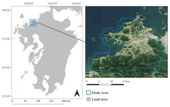
Figure 1.
Location of the study area. A composite image of Sentinel-2 data was used for visualization. The land area was provided by the National Land Numerical Information (http://nlftp.mlit.go.jp/ksj-e/index.html).
2.2. Airborne LiDAR Data
Wall-to-wall airborne LiDAR data were acquired from 31 January to 5 February 2016, using a Trimble Harrier 68i laser system mounted on the rotary-wing helicopter with a flight altitude of 400 m. The average pulse density was 23.5 pulses per m2. Ground control points in the study area were used for data registration. The point cloud data were classified into ground and non-ground classes using a cloth simulation filtering algorithm [25]. A digital terrain model (DTM) was generated with spatial interpolation of the ground points using a triangle irregular network (TIN) at a spatial resolution of 0.25 m. All LiDAR point clouds were normalized using the DTM. The mean canopy height (MCH) was calculated at spatial resolutions of 3, 10, 20, and 30 m. Manipulation of the LiDAR point data was conducted using the “lidR” package [26] in the R statistical software [27].
2.3. PlanetScope, Landsat 8, and Sentinel-2 Data
PlanetScope Analytic Ortho Scene surface reflectance (SR) Level 3B data were used in this study. This data product has four spectral bands (blue, green, red, and near-infrared) with a spatial resolution resampled at 3 m [19]. All PlanetScope data were acquired in 2017 with less than 50% cloud cover. A visual interpretation was conducted to remove low-quality data and images affected by haze. The porder tool [28] was used to list, order, and download the PlanetScope data through the Planet Application Program Interface [29]. Clouds were masked using an Automatic Time-Series Analysis algorithm [30]. Several studies have reported radiometric consistency issues in the PlanetScope SR data due to cross-sensor inconsistency [31,32]. However, in this study, we considered the radiometric correction of PlanetScope SR data to be sufficient. This is because our preliminary analysis confirmed that the distribution of root mean squared error (RMSE) of the actual and predicted values from the first-order harmonic regression model applied to PlanetScope’s time series spectral bands was in the range of that of the Landsat 8 and Sentinel-2 data (Figure 2). This indicated that the variability of SR values in PlanetScope data due to atmospheric effects was similar to Landsat 8 and Sentinel-2. Therefore, no additional preprocessing was applied to the PlanetScope SR data. All four spectral bands were used for further analyses. A total of 148 images across 35 days were used (Table 1).
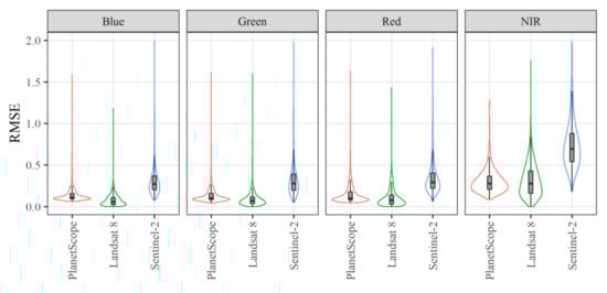
Figure 2.
The distribution of the RMSE of the actual and predicted values from the first-order harmonic regression model applied to four spectral bands (blue, green red, and near-infrared) for each satellite data.

Table 1.
The number of images, days, and average valid pixels for PlanetScope, Landsat 8, and Sentinel-2 data from 2017. The average valid pixels were calculated as the average number of cloud-free observations in each pixel location.
Landsat 8 Operational Land Imager Collection 1 SR data were downloaded from the Google Earth Engine [33]. Data from the study area that were acquired between the beginning of 2016 and the end of 2018 with less than 50% cloud cover were used. The Landsat 8 SR data were atmospherically corrected by the LaSRC [34]. Clouds and cloud shadows were masked using a pixel QA band from the CFmask algorithm [35,36]. A total of 45 images from 45 days from 2016 to 2018 were used, including 15 images from 15 days in 2017 (Figure 3). A total of six spectral bands (band 2, 3, 4, 5, 6, and 7) were used.
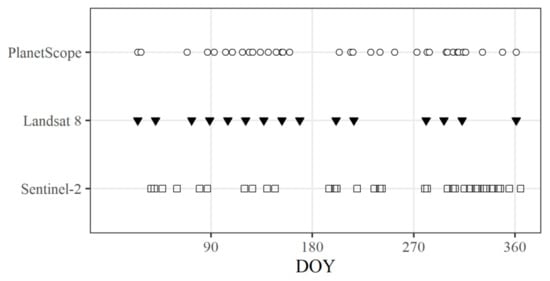
Figure 3.
The day of year (DOY) of images used for each satellite data. The images acquired on the same date were plotted as one observation.
Sentinel-2 Multispectral Instrument Level 1C data acquired in 2017 were used, where cloud cover was less than 50%. The Level 1C top of atmosphere (TOA) reflectance data in the Long Term Archive of the European Space Agency Copernicus Open Access Hub were ordered and downloaded using the “sen2r” package [37]. All Level 1C data were corrected to bottom of atmosphere (BOA) reflectance data using the Sen2Cor algorithm [38]. Clouds and cloud shadows were masked using the scene classification map computed by Sen2Cor. As a result of Sen2Cor processing, band 8a and 10 were removed at the BOA reflectance data. In addition, 60 m spatial resolution bands were removed in this study because these bands were mainly dedicated for atmospheric correction and cloud detection [39]. All remaining spectral bands of BOA reflectance data (band 2, 3, 4, 5, 6, 7, 8, 11, and 12) were resampled to a spatial resolution of 10 m. A total of 58 images from 33 days were used (Table 1 and Figure 3).
2.4. Predictor Variables from PlanetScope, Landsat 8, and Sentinel-2 Data
We prepared a suite of images corresponding to single composite, multi-seasonal composites, and time-series data to derive predictor variables from each satellite data (i.e., PlanetScope, Landsat 8, and Sentinel-2) at spatial resolutions of 3, 10, 20, and 30 m. All PlanetScope, Landsat 8 and Sentinel-2 data were first resampled and co-registered to LiDAR MCH pixels (i.e., 3, 10, 20, and 30 m) using bilinear interpolation. The single composite was generated by calculating the median composite of all 2017 images. The multi-seasonal composites were generated from the median composite of images acquired in winter (January to March), spring (April to June), summer (July to September), and autumn (October to December). For Landsat 8 only, images from 2016 to 2018 were used to generate multi-seasonal composites to avoid missing pixels. The time-series data were generated from all images in 2017.
Predictor variables were extracted from a suite of images (Table 2). Spectral bands, the Normalized Difference Vegetation Index (NDVI), Normalized Difference Moisture Index (NDMI), Normalized Burn Ratio (NBR), Enhanced Vegetation Index (EVI), and the Gray Level Co-occurrence Matrix (GLCM) were used as predictor variables from the single composite. A total of seven first- and second-order texture measures (mean, variance, homogeneity, contrast, dissimilarity, entropy, and second moment) were calculated as GLCM variables within a 3 × 3 pixel window. The near-infrared band was selected to calculate the GLCM. We calculated the same predictor variables as the single composite for spring, summer, autumn, and winter multi-seasonal composites. The harmonic regression model was fitted to all spectral bands and the indices of time-series data using the following equation [40]:
where is the time of data acquired, is the constant term, and are the first-order amplitude of cosine and sine waves, respectively, and and are the second-order amplitude of cosine and sine waves, respectively. We used a first-order harmonic regression model for Landsat 8 due to the limited number of available images, whereas Equation (1) was used for PlanetScope and Sentinel-2. These coefficients were used as predictor variables in modeling with time-series data. In addition, the RMSEs of harmonic regression and the mean observation values were included as predictor variables.
Table 2.
The predictor variables and number of variables investigated in each set of processing and satellite data. These variables are the same regardless of the spatial resolution.
2.5. Random Forest Model Building
To build random forest (RF) models [41] for estimating airborne LiDAR derived MCH, training and test sample pixels were extracted from the study area. Prior to sampling the pixels, water bodies were excluded using a global surface water mask [42]. In addition, because forest disturbances that had occurred between the airborne LiDAR data acquisition and the satellite data could potentially influence the RF model development, we excluded the disturbance areas in 2016 and 2017 using Hansen Global Forest Change data [43]. After eliminating the water bodies and disturbed pixels, we randomly selected 5000 pixels for both training and test samples, which were first derived from the MCH pixels at 3 m spatial resolution. The same sample locations were then used for other spatial resolutions to minimize possible sampling errors. In cases where multiple samples were located in the same pixel at resolutions of 10, 20, and 30 m, we simply left one sample at each pixel.
For each RF model, feature selection was implemented to reduce redundant information in predictor variables using the “ClustOfVar” package [44]. This algorithm is based on a hierarchical clustering method and identifies the cluster of variables using the squared Pearson correlation for quantitative variables. The optimal number of clusters was determined using the adjusted Rand index [45]. One predictor variable was then selected from each cluster.
The RF models were developed for all PlanetScope, Landsat 8, and Sentinel-2 processing sets across all spatial resolutions using the “randomForest” package [46]. The models were tuned with 10-fold cross validation of 500 trees using the “caret” package [47]. The developed RF models were applied to test samples to evaluate the estimation accuracy. The coefficient of determination (R2), RMSE, and relative RMSE (rRMSE) were used for accuracy assessment, which were expressed as follows:
where is the LiDAR MCH of the ith test sample, is the mean value of LiDAR MCH, is the predicted MCH of the ith test sample, and is the number of test samples.
Accuracy was also assessed based on forest and non-forest classes. The class was determined using a forest area layer from the National Land Numerical Information (http://nlftp.mlit.go.jp/ksj-e/index.html). The developed RF models were applied to the entire study area to map the canopy height. The variable importance was calculated based on the mean decrease in accuracy.
3. Results
3.1. Accuracy Assessment of RF Models
A total of 36 RF models were developed based on predictor variables from different satellite data (PlanetScope, Landsat 8, and Sentinel-2), processing sets (single composite, multi-seasonal composites, and time series), and spatial resolutions (3, 10, 20, and 30 m), and the accuracy of estimating airborne LiDAR derived MCH was evaluated. The RMSE ranged from 2.56 (rRMSE, 36.1%) to 3.97 m (57.4%), from 2.63 (37.2%) to 4.01 m (58.2%), and from 2.40 (34.2%) to 3.76 m (55.0%) for PlanetScope, Landsat 8, and Sentinel-2, respectively (Figure 4a). The lower rRMSEs were found in the RF models with a lower spatial resolution across all satellite data and processing sets. When the rRMSE was assessed in the forest and non-forest classes, rRMSE values in the forest class were lower than those in the non-forest class for all RF models (Figure 4b,c). Similar trends were observed for R2, ranging from 0.62 to 0.81, 0.61 to 0.80, and 0.66 to 0.83 for PlanetScope, Landsat 8, and Sentinel-2, respectively (Figure 5). For 3 m spatial resolution, the lowest rRMSE and highest R2 were achieved by an RF model with PlanetScope multi-seasonal composites (rRMSE of 51.3% and an R2 of 0.70). For the other spatial resolutions, these were achieved by Sentinel-2 multi-seasonal composites (rRMSE of 40.5%, 35.2%, and 34.2% for 10, 20, and 30 m, respectively, and an R2 of 0.79, 0.83, and 0.83 for 10, 20, and 30 m, respectively). The highest R2 (0.83) and the lowest RMSE (2.40 m) and rRMSE (34.2%) were obtained by an RF model with the Sentinel-2 multi-seasonal composites resampled to 30 m.
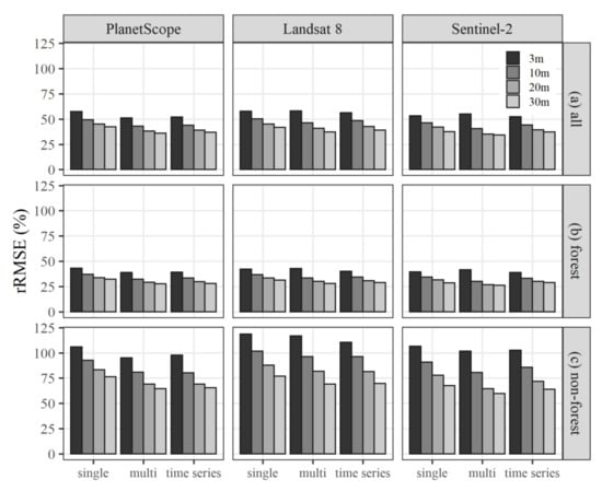
Figure 4.
rRMSE of random forest (RF) models from different combinations of satellite data (PlanetScope, Landsat 8, and Sentinel-2), processing sets (single composite, multi-seasonal composites, and time series), and spatial resolutions (3, 10, 20, and 30 m) in (a) all, (b) forest, and (c) non-forest classes.
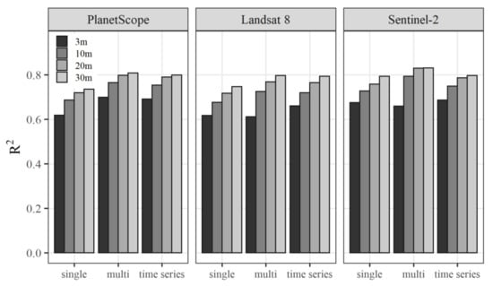
Figure 5.
R2 of RF models from different combinations of satellite data (PlanetScope, Landsat 8, and Sentinel-2), processing sets (single composite, multi-seasonal composites, and time series), and spatial resolutions (3, 10, 20, and 30 m).
Table 3 summarizes the differences between rRMSE and R2 for RF models with different satellite data, processing, and spatial resolutions. The lower rRMSEs and higher R2 were found in RF models with a lower spatial resolution; however, the differences became smaller with decreasing spatial resolution (rRMSE, −8.0%, −5.0%, and −2.7% for 3 to 10 m, 10 to 20 m, and 20 to 30 m, respectively; R2, 0.06, 0.04, and 0.02 for 3 to 10 m, 10 to 20 m, and 20 to 30 m, respectively). In terms of processing, RF models using multi-seasonal composites exhibited a slightly better prediction accuracy compared with those using time-series data (−1.4% and 0.01 for rRMSE and R2, respectively), followed by those using a single composite. When the prediction accuracy was assessed based on satellite data, the RF models with Sentinel-2 achieved lower rRMSEs and a higher R2 compared with PlanetScope (−2.2% and 0.03 for rRMSE and R2, respectively) and Landsat 8 (−4.0% and 0.04 for rRMSE and R2, respectively).
Table 3.
Median, minimum, and maximum values of the differences between the prediction accuracy of RF models for each combination, in terms of rRMSE and R2. The comparison was based on combinations of (1) the same satellite data and processing, (2) the same satellite data and spatial resolution, and (3) the same spatial resolution and processing.
Figure 6 shows the scatter plots of the predicted and airborne LiDAR MCH. The underestimation of MCH in higher canopy height was observed in all RF models, even though this was alleviated in some cases. In addition, the predicted MCH values were also overestimated in lower canopy height, especially those with 3 m spatial resolution.
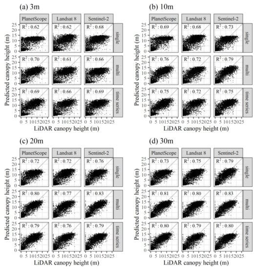
Figure 6.
Scatter plots of the predicted and LiDAR mean canopy height (MCH) at spatial resolutions of (a) 3 m, (b) 10 m, (c) 20 m, and (d) 30 m for different combinations of satellite data and processing.
The five most important variables in each RF model were shown in Table 4. Although variable importance varied at different spatial resolutions, several predictor variables were ranked as the five most important variables regardless of spatial resolution (e.g., b5 in Landsat 8 single composite, NBR-mean in Sentinel-2 time series, and summer-NDVI in PlanetScope multi-seasonal composites). In the RF models using time-series data, variables from harmonic regression models were important variables although the mean values of spectral bands and indices had the highest importance in all models. The GLCM variables were important variables in all spatial resolutions of RF models using PlanetScope single composite. The near-infrared and short-wave infrared related spectral bands and indices had the highest importance in 29 out of 36 RF models.
Table 4.
The five most important variables in RF models at spatial resolutions of (a) 3 m, (b) 10 m, (c) 20 m, and (d) 30 m for different combinations of satellite data and processing.
3.2. MCH Mapping
Figure 7 shows an example of MCH mapping from the PlanetScope multi-seasonal composites at 3 m for the entire study area. Figure 8 shows a detailed example of MCH mapping in the study area, which includes forest roads and harvested areas with stripe shapes, using multi-seasonal composites at different spatial resolutions. The mapped canopy height was different for each combination of satellite data and spatial resolution. It was visually difficult to map the MCH in small-scale disturbed areas, especially with 3 m spatial resolution, leading to obscured mapping to small paths and harvested areas. The canopy heights with a lower spatial resolution had better visualization of these small-scale disturbance areas; however, they were not clear at 30 m spatial resolution.
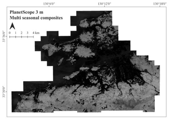
Figure 7.
Example of MCH mapping from the PlanetScope multi-seasonal composites at 3 m for the entire study area.
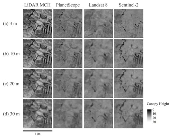
Figure 8.
Example of MCH mapping for subsets from airborne LiDAR and RF models at different spatial resolutions. The estimation of RF models using multi-seasonal composites of (a) 3 m, (b) 10 m, (c) 20 m, and (d) 30 m are shown.
4. Discussion
The single composite, multi-seasonal composites, and time-series RF models had varying accuracies for different combinations of satellite data and spatial resolution. Although the RF models with time-series data performed better than those with multi-seasonal composites in some combinations (e.g., Landsat 8 with 3 m), the multi-seasonal composites generally had higher prediction accuracy. Previous studies have indicated the effectiveness of using textural variables, which are good indicators of vegetation structure as well as spatial characteristics of tree canopies [48], to estimate growing stock volumes [49]. The seasonal information from multi-temporal images was also effective for estimating forest structural attributes in previous studies [8,49,50], the results of which are consistent with those in this study. This might be explained by lower canopy height in broadleaf forests in the study area. Because seasonal and phenological variation in evergreen broadleaf forests in this region can be distinguished by satellite data [51], the RF models using multi-seasonal composites might have higher accuracies. In contrast, as noted by Csillik et al. [24], the contribution of textural information from the PlanetScope data is not apparent and needs further investigation. Several studies have used harmonic metrics from time-series data to classify tree species and estimate canopy cover (e.g., [40,52,53]). This has been found to be more accurate compared with multi-seasonal composites [54]; however, improvements using harmonic metrics were not observed when estimating canopy height in this study. This was potentially caused by undetected cloudy pixels in time-series data.
The PlanetScope estimations achieved the highest accuracy with a 3 m spatial resolution. Downscaling the Sentinel-2 and Landsat 8 data to 3 m does not result in any new information; therefore, it is sensible to use PlanetScope data with a 3 m spatial resolution to improve prediction accuracy. At a spatial resolution of less than 10 m, the RF models with Sentinel-2 achieved the highest accuracy. The potential of short-wave infrared and red-edge bands of Sentinel-2 for forest structural mapping has been demonstrated in previous studies [9,55]. This may be one of the reasons why Sentinel-2 is more accurate than PlanetScope, which has only four spectral bands. This was supported by high variable importance of short-wave infrared related variables in Sentinel-2. Although the original spatial resolution of the PlanetScope data is higher than that of Sentinel-2, the RF models with Sentinel-2 were more accurate. The influential factor for the lower accuracy achieved by Landsat 8 may be its lower original spatial resolution compared with PlanetScope and Sentinel-2. A previous study showed that the spectral indices from PlanetScope did not have a significant contribution to forest structural estimates in tropical forests [23]. This might be caused by different vegetation conditions and should be investigated in further studies.
In general, the RF models with a lower spatial resolution had a higher prediction accuracy (Figure 4 and Figure 5). This is partially explained by the reduced co-registration errors between airborne LiDAR derived MCH and satellite observation [20]. As the errors in estimating AGB from tree height decrease with a lower spatial resolution [56] due to a slower rate of increasing total error than total AGB, our study may also be affected by spatial error variations in estimating canopy heights at different spatial resolutions.
All RF models showed an underestimation of canopy heights at higher values. The underestimation of canopy heights using optical satellite data was reported in other studies (e.g., [57]), and this is explained by the saturation of reflectance at a certain height. The overestimation of low canopy heights was partially caused by low prediction accuracy in small areas that had low or zero canopy height, as shown in Figure 8. Temporal differences between data acquisition may be another reason due to vegetation recovery after forest disturbance. One possible solution for reducing prediction biases could come from investigations into alternative machine learning approaches, such as deep learning (e.g., [10]).
In this study, we only investigated the use of optical satellite data; however, other types of satellite data, such as SAR data, might be used for accurate canopy height mapping. Because SAR can observe the forest structure even in cloudy conditions, frequent observation can be achieved by SAR data for regional and countrywide scale monitoring. Although L-band SAR observations are sometimes limited by the availability of the operational L-band SAR satellite (i.e., ALOS-2/PALSAR-2), the Copernicus Sentinel-1 mission provides temporally dense and systematically acquired C-band SAR data since launched in 2014. Previous studies have used ALOS-2 and Sentinel-1 data for forest structural estimation (e.g., [23,55]), and showed the potential use of SAR data. Further studies might investigate the integration of optical and SAR satellite data for estimating forest structural attributes.
CubeSat data, such as those from PlanetScope, has great potential to map forest structural attributes in conjunction with field surveys and airborne LiDAR data on a regional and countrywide scale at a reasonable cost. This study found that PlanetScope performed well with a fine spatial resolution of 3 m; however, Sentinel-2 was more accurate for other spatial resolutions using multi-seasonal composites. Sentinel-2 might be more applicable for large scale monitoring, while PlanetScope might be used for near-real-time and detailed monitoring. In addition, because of the high spatial and temporal resolution of the PlanetScope data, robust forest monitoring using PlanetScope data, such as the near-real-time monitoring of forest attributes with a finer spatial resolution, may be possible. Future research is needed to study the various applications in different forest types.
5. Conclusions
This study examined the capabilities of PlanetScope data to map canopy heights and compared this with the performance of Landsat 8 and Sentinel-2 data in temperate forests. Previous studies have rarely investigated the predictive features from multi-seasonal composites and time series of PlanetScope data. This study systematically evaluated the relative performance of RF models from these variables. The accuracy of RF models for estimating airborne LiDAR derived MCH indicated that PlanetScope data was suitable for mapping at 3 m spatial resolution with an rRMSE of 51.3% and an R2 of 0.70; however, for lower spatial resolutions (10, 20, and 30 m), RF models using Sentinel-2 data performed better. The RF models using multi-seasonal composites achieved a higher prediction accuracy compared with those using time-series data or a single composite. PlanetScope data is recommended for use with finer spatial resolution; however, considering the minor differences between the prediction accuracies of Sentinel-2 and PlanetScope, and the high spatial and temporal resolution of PlanetScope, further uses of PlanetScope data, such as near-real-time monitoring, should be investigated.
Author Contributions
Conceptualization, K.S.; methodology, K.S., T.O., and N.M.; software, K.S.; validation, K.S.; investigation, K.S.; resources, K.S., T.O., and N.M.; data curation, K.S., T.O., and N.M.; writing—original draft preparation, K.S.; writing—review and editing, K.S., T.O., N.M., and H.S.; visualization, K.S.; supervision, H.S. All authors have read and agreed to the published version of the manuscript.
Funding
This research received no external funding.
Acknowledgments
We thank Itoshima City for giving the access to airborne LiDAR data. Planet data were provided through the Planet Education and Research program. We thank the anonymous reviewers for their constructive comments.
Conflicts of Interest
The authors declare no conflict of interest.
References
- Skovsgaard, J.P.; Vanclay, J.K. Forest site productivity: A review of the evolution of dendrometric concepts for even-aged stands. For. Int. J. For. Res. 2008, 81, 13–31. [Google Scholar] [CrossRef]
- Skidmore, A.K.; Pettorelli, N.; Coops, N.C.; Geller, G.N.; Hansen, M.; Lucas, R.; Mücher, C.A.; O’Connor, B.; Paganini, M.; Pereira, H.M.; et al. Environmental science: Agree on biodiversity metrics to track from space. Nature 2015, 523, 403–405. [Google Scholar] [CrossRef]
- Asner, G.P.; Mascaro, J. Mapping tropical forest carbon: Calibrating plot estimates to a simple LiDAR metric. Remote Sens. Environ. 2014, 140, 614–624. [Google Scholar] [CrossRef]
- Wulder, M.A.; White, J.C.; Nelson, R.F.; Næsset, E.; Ørka, H.O.; Coops, N.C.; Hilker, T.; Bater, C.W.; Gobakken, T. Lidar sampling for large-area forest characterization: A review. Remote Sens. Environ. 2012, 121, 196–209. [Google Scholar] [CrossRef]
- Wilkes, P.; Jones, S.; Suarez, L.; Mellor, A.; Woodgate, W.; Soto-Berelov, M.; Haywood, A.; Skidmore, A. Mapping Forest Canopy Height Across Large Areas by Upscaling ALS Estimates with Freely Available Satellite Data. Remote Sens. 2015, 7, 12563–12587. [Google Scholar] [CrossRef]
- Ota, T.; Ahmed, O.S.; Franklin, S.; Wulder, M.; Kajisa, T.; Mizoue, N.; Yoshida, S.; Takao, G.; Hirata, Y.; Furuya, N.; et al. Estimation of Airborne Lidar-Derived Tropical Forest Canopy Height Using Landsat Time Series in Cambodia. Remote Sens. 2014, 6, 10750–10772. [Google Scholar] [CrossRef]
- Staben, G.; Lucieer, A.; Scarth, P. Modelling LiDAR derived tree canopy height from Landsat TM, ETM+ and OLI satellite imagery—A machine learning approach. Int. J. Appl. Earth Obs. Geoinf. 2018, 73, 666–681. [Google Scholar] [CrossRef]
- Chrysafis, I.; Mallinis, G.; Tsakiri, M.; Patias, P. Evaluation of single-date and multi-seasonal spatial and spectral information of Sentinel-2 imagery to assess growing stock volume of a Mediterranean forest. Int. J. Appl. Earth Obs. Geoinf. 2019, 77, 1–14. [Google Scholar] [CrossRef]
- Astola, H.; Häme, T.; Sirro, L.; Molinier, M.; Kilpi, J. Comparison of Sentinel-2 and Landsat 8 imagery for forest variable prediction in boreal region. Remote Sens. Environ. 2019, 223, 257–273. [Google Scholar] [CrossRef]
- Lang, N.; Schindler, K.; Wegner, J.D. Country-wide high-resolution vegetation height mapping with Sentinel-2. Remote Sens. Environ. 2019, 233, 111347. [Google Scholar] [CrossRef]
- Matasci, G.; Hermosilla, T.; Wulder, M.A.; White, J.C.; Coops, N.C.; Hobart, G.W.; Zald, H.S.J. Large-area mapping of Canadian boreal forest cover, height, biomass and other structural attributes using Landsat composites and lidar plots. Remote Sens. Environ. 2018, 209, 90–106. [Google Scholar] [CrossRef]
- Hirata, Y.; Furuya, N.; Saito, H.; Pak, C.; Leng, C.; Sokh, H.; Ma, V.; Kajisa, T.; Ota, T.; Mizoue, N. Object-Based Mapping of Aboveground Biomass in Tropical Forests Using LiDAR and Very-High-Spatial-Resolution Satellite Data. Remote Sens. 2018, 10, 438. [Google Scholar] [CrossRef]
- Finer, M.; Novoa, S.; Weisse, J.; Petersen, R.; Souto, T.; Stearns, F.; Martinez, R.G. Combating deforestation: From satellite to intervention. Science 2018, 360, 1303–1305. [Google Scholar] [CrossRef]
- Fagua, J.C.; Jantz, P.; Rodriguez-Buritica, S.; Duncanson, L.; Goetz, S.J. Integrating LiDAR, Multispectral and SAR Data to Estimate and Map Canopy Height in Tropical Forests. Remote Sens. 2019, 11, 2697. [Google Scholar] [CrossRef]
- Mura, M.; Bottalico, F.; Giannetti, F.; Bertani, R.; Giannini, R.; Mancini, M.; Orlandini, S.; Travaglini, D.; Chirici, G. Exploiting the capabilities of the Sentinel-2 multi spectral instrument for predicting growing stock volume in forest ecosystems. Int. J. Appl. Earth Obs. Geoinf. 2018, 66, 126–134. [Google Scholar] [CrossRef]
- Bolton, D.K.; White, J.C.; Wulder, M.A.; Coops, N.C.; Hermosilla, T.; Yuan, X. Updating stand-level forest inventories using airborne laser scanning and Landsat time series data. Int. J. Appl. Earth Obs. Geoinf. 2018, 66, 174–183. [Google Scholar] [CrossRef]
- Bolton, D.K.; Gray, J.M.; Melaas, E.K.; Moon, M.; Eklundh, L.; Friedl, M.A. Continental-scale land surface phenology from harmonized Landsat 8 and Sentinel-2 imagery. Remote Sens. Environ. 2020, 240, 111685. [Google Scholar] [CrossRef]
- Poghosyan, A.; Golkar, A. CubeSat evolution: Analyzing CubeSat capabilities for conducting science missions. Prog. Aerosp. Sci. 2017, 88, 59–83. [Google Scholar] [CrossRef]
- Planet Team. Planet Imagery Product Specifications; Planet: San Francisco, CA, USA, 2020. [Google Scholar]
- Riihimäki, H.; Luoto, M.; Heiskanen, J. Estimating fractional cover of tundra vegetation at multiple scales using unmanned aerial systems and optical satellite data. Remote Sens. Environ. 2019, 224, 119–132. [Google Scholar] [CrossRef]
- Csillik, O.; Kumar, P.; Mascaro, J.; O’Shea, T.; Asner, G.P. Monitoring tropical forest carbon stocks and emissions using Planet satellite data. Sci. Rep. 2019, 9, 17831. [Google Scholar] [CrossRef]
- Baloloy, A.B.; Blanco, A.C.; Candido, C.G.; Argamosa, R.J.L.; Dumalag, J.B.L.C.; Dimapilis, L.L.C.; Paringit, E.C. Estimation of mangrove forest aboveground biomass using multispectral bands, vegetation indices and biophysical variables derived from optical satellite imageries: RapidEye, Planetscope and Sentinel-2. ISPRS Ann. Photogramm. Remote Sens. Spat. Inf. Sci. 2018, IV-3, 29–36. [Google Scholar] [CrossRef]
- Mulatu, K.A.; Decuyper, M.; Brede, B.; Kooistra, L.; Reiche, J.; Mora, B.; Herold, M. Linking Terrestrial LiDAR Scanner and Conventional Forest Structure Measurements with Multi-Modal Satellite Data. Forests 2019, 10, 291. [Google Scholar] [CrossRef]
- Csillik, O.; Kumar, P.; Asner, G.P. Challenges in Estimating Tropical Forest Canopy Height from Planet Dove Imagery. Remote Sens. 2020, 12, 1160. [Google Scholar] [CrossRef]
- Zhang, W.; Qi, J.; Wan, P.; Wang, H.; Xie, D.; Wang, X.; Yan, G. An Easy-to-Use Airborne LiDAR Data Filtering Method Based on Cloth Simulation. Remote Sens. 2016, 8, 501. [Google Scholar] [CrossRef]
- Roussel, J.-R.; Auty, D. lidR: Airborne LiDAR Data Manipulation and Visualization for Forestry Applications. 2020. Available online: https://cran.r-project.org/web/packages/lidR/index.html (accessed on 6 April 2020).
- R Core Team. R: A Language and Environment for Statistical Computing; R Foundation for Statistical Computing: Vienna, Austria, 2019. [Google Scholar]
- Roy, S. Porder: Simple CLI for Planet Orders V2 API. 2020. Available online: https://zenodo.org/record/3875911 (accessed on 6 April 2020).
- Planet Team. Planet Application Program Interface: In Space for Life on Earth; Planet: San Francisco, CA, USA, 2018. [Google Scholar]
- Zhu, X.; Helmer, E.H. An automatic method for screening clouds and cloud shadows in optical satellite image time series in cloudy regions. Remote Sens. Environ. 2018, 214, 135–153. [Google Scholar] [CrossRef]
- Leach, N.; Coops, N.C.; Obrknezev, N. Normalization method for multi-sensor high spatial and temporal resolution satellite imagery with radiometric inconsistencies. Comput. Electron. Agric. 2019, 164, 104893. [Google Scholar] [CrossRef]
- Houborg, R.; McCabe, M. Daily Retrieval of NDVI and LAI at 3 m Resolution via the Fusion of CubeSat, Landsat, and MODIS Data. Remote Sens. 2018, 10, 890. [Google Scholar] [CrossRef]
- Gorelick, N.; Hancher, M.; Dixon, M.; Ilyushchenko, S.; Thau, D.; Moore, R. Google Earth Engine: Planetary-scale geospatial analysis for everyone. Remote Sens. Environ. 2017. [Google Scholar] [CrossRef]
- Vermote, E.; Justice, C.; Claverie, M.; Franch, B. Preliminary analysis of the performance of the Landsat 8/OLI land surface reflectance product. Remote Sens. Environ. 2016, 185, 46–56. [Google Scholar] [CrossRef]
- Zhu, Z.; Woodcock, C.E. Object-based cloud and cloud shadow detection in Landsat imagery. Remote Sens. Environ. 2012, 118, 83–94. [Google Scholar] [CrossRef]
- Zhu, Z.; Wang, S.; Woodcock, C.E. Improvement and expansion of the Fmask algorithm: Cloud, cloud shadow, and snow detection for Landsats 4–7, 8, and Sentinel 2 images. Remote Sens. Environ. 2015, 159, 269–277. [Google Scholar] [CrossRef]
- Ranghetti, L.; Boschetti, M.; Nutini, F.; Busetto, L. “sen2r”: An R toolbox for automatically downloading and preprocessing Sentinel-2 satellite data. Comput. Geosci. 2020, 139, 104473. [Google Scholar] [CrossRef]
- Main-Knorn, M.; Pflug, B.; Louis, J.; Debaecker, V.; Müller-Wilm, U.; Gascon, F. Sen2Cor for Sentinel-2. In Proceedings of the Image and Signal Processing for Remote Sensing XXIII, Warsaw, Poland, 11–13 September 2017; Bruzzone, L., Bovolo, F., Benediktsson, J.A., Eds.; SPIE: Warsaw, Poland, 2017; 10427, p. 1042704. [Google Scholar]
- Drusch, M.; Del Bello, U.; Carlier, S.; Colin, O.; Fernandez, V.; Gascon, F.; Hoersch, B.; Isola, C.; Laberinti, P.; Martimort, P.; et al. Sentinel-2: ESA’s Optical High-Resolution Mission for GMES Operational Services. Remote Sens. Environ. 2012, 120, 25–36. [Google Scholar] [CrossRef]
- Derwin, J.M.; Thomas, V.A.; Wynne, R.H.; Coulston, J.W.; Liknes, G.C.; Bender, S.; Blinn, C.E.; Brooks, E.B.; Ruefenacht, B.; Benton, R.; et al. Estimating tree canopy cover using harmonic regression coefficients derived from multitemporal Landsat data. Int. J. Appl. Earth Obs. Geoinf. 2020, 86, 101985. [Google Scholar] [CrossRef]
- Breiman, L. Random forests. Mach. Learn. 2001, 45, 5–32. [Google Scholar] [CrossRef]
- Pekel, J.-F.; Cottam, A.; Gorelick, N.; Belward, A.S. High-resolution mapping of global surface water and its long-term changes. Nature 2016, 540, 418–422. [Google Scholar] [CrossRef]
- Hansen, M.C.; Potapov, P.V.; Moore, R.; Hancher, M.; Turubanova, S.A.; Tyukavina, A.; Thau, D.; Stehman, S.V.; Goetz, S.J.; Loveland, T.R.; et al. High-Resolution Global Maps of 21st-Century Forest Cover Change. Science 2013, 342, 850–853. [Google Scholar] [CrossRef]
- Chavent, M.; Kuentz-Simonet, V.; Liquet, B.; Saracco, J. ClustOfVar: An R package for the clustering of variables. J. Stat. Softw. 2012, 50, 1–16. [Google Scholar] [CrossRef]
- Hubert, L.; Arabie, P. Comparing partitions. J. Classif. 1985, 2, 193–218. [Google Scholar] [CrossRef]
- Liaw, A.; Wiener, M. Classification and regression by randomForest. R News 2002, 2, 18–22. [Google Scholar]
- Kuhn, M. Building predictive models in R using the caret package. J. Stat. Softw. 2008, 28, 1–26. [Google Scholar] [CrossRef]
- Wood, E.M.; Pidgeon, A.M.; Radeloff, V.C.; Keuler, N.S. Image texture as a remotely sensed measure of vegetation structure. Remote Sens. Environ. 2012, 121, 516–526. [Google Scholar] [CrossRef]
- Sánchez-Ruiz, S.; Moreno-Martínez, Á.; Izquierdo-Verdiguier, E.; Chiesi, M.; Maselli, F.; Gilabert, M.A. Growing stock volume from multi-temporal landsat imagery through google earth engine. Int. J. Appl. Earth Obs. Geoinf. 2019, 83, 101913. [Google Scholar] [CrossRef]
- Chrysafis, I.; Mallinis, G.; Gitas, I.; Tsakiri-Strati, M. Estimating Mediterranean forest parameters using multi seasonal Landsat 8 OLI imagery and an ensemble learning method. Remote Sens. Environ. 2017, 199, 154–166. [Google Scholar] [CrossRef]
- Murakami, T. Seasonal variation in classification accuracy of forest-cover types examined by a single band or band combinations. J. For. Res. 2004, 9, 211–215. [Google Scholar] [CrossRef]
- Wilson, B.T.; Knight, J.F.; McRoberts, R.E. Harmonic regression of Landsat time series for modeling attributes from national forest inventory data. ISPRS J. Photogramm. Remote Sens. 2018, 137, 29–46. [Google Scholar] [CrossRef]
- Cheng, K.; Wang, J. Forest Type Classification Based on Integrated Spectral-Spatial-Temporal Features and Random Forest Algorithm—A Case Study in the Qinling Mountains. Forests 2019, 10, 559. [Google Scholar] [CrossRef]
- Adams, B.; Iverson, L.; Matthews, S.; Peters, M.; Prasad, A.; Hix, D. Mapping Forest Composition with Landsat Time Series: An Evaluation of Seasonal Composites and Harmonic Regression. Remote Sens. 2020, 12, 610. [Google Scholar] [CrossRef]
- Mauya, E.W.; Koskinen, J.; Tegel, K.; Hämäläinen, J.; Kauranne, T.; Käyhkö, N. Modelling and Predicting the Growing Stock Volume in Small-Scale Plantation Forests of Tanzania Using Multi-Sensor Image Synergy. Forests 2019, 10, 279. [Google Scholar] [CrossRef]
- Mascaro, J.; Detto, M.; Asner, G.P.; Muller-Landau, H.C. Evaluating uncertainty in mapping forest carbon with airborne LiDAR. Remote Sens. Environ. 2011, 115, 3770–3774. [Google Scholar] [CrossRef]
- Hansen, M.C.; Potapov, P.V.; Goetz, S.J.; Turubanova, S.; Tyukavina, A.; Krylov, A.; Kommareddy, A.; Egorov, A. Mapping tree height distributions in Sub-Saharan Africa using Landsat 7 and 8 data. Remote Sens. Environ. 2016, 185, 221–232. [Google Scholar] [CrossRef]
© 2020 by the authors. Licensee MDPI, Basel, Switzerland. This article is an open access article distributed under the terms and conditions of the Creative Commons Attribution (CC BY) license (http://creativecommons.org/licenses/by/4.0/).