Landscape Patterns and Building Functions for Urban Land-Use Classification from Remote Sensing Images at the Block Level: A Case Study of Wuchang District, Wuhan, China

Abstract

Landscape patterns and building functions are successfully used to provide the social sensing information of urban areas. However, previous studies treated ground objects equally, ignoring their size differences. Considering the different contributions of various types of ground objects in land-use classification, this paper measured nine area-weighted mean landscape-level metrics to describe landscape patterns based on the land-cover map, derived from remote sensing images. Additionally, the same idea was applied for identifying building functions. Impervious surfaces, which occupy the majority of urban areas, have a decisive impact on land-use classes. In terms of this, this paper proposed the impervious surface area-weighted building-based indexes from the building outline data. To better represent the physical structure of urban areas, the entire study was based on the analysis units delineated by the OpenStreetMap road network. Finally, a random forest model combining the landscape-level metrics and building-based indexes was adopted in Wuchang District of Wuhan city, China. The results showed that the proposed method was effective at describing landscape patterns and identifying building functions for accurate urban land-use classification, increasing the precision by 10.67%. In general, the contribution of landscape-level metrics to the urban land-use classification is slightly greater than that of building-based indexes. Moreover, different land-use types of analysis units express different landscape patterns. It is of great significance for improving urban form and guiding future urban design. The paper demonstrates that area-weighted landscape metrics and building-based indexes offer a better understanding of urban land use, which plays a vital role in urban planning, construction, and management.

1. Introduction

In fast-growing countries, like China, the urban land use is changing rapidly. To quantitatively characterize the land-use classes is essential for planners and policymakers [1,2]. However, traditional data collection methods, such as censuses or land-use surveys, are time-consuming, labor-intensive, error-prone, and costly [3]. The emergence of remote sensing images makes it possible for urban planners to collect exhaustive land-cover information and to characterize the current land use on a smaller time scale and cost-effectively [4,5]. Early studies focused on the physical characteristics of remote sensing data to classify urban areas. Then, with more and more emphasis on the socioeconomic attribute of cities, researchers not only added the landscape pattern of remote sensing images to represent the interactions between human activities and their living environment, but also connected remote sensing information with social sensing information to map urban areas comprehensively.

The idea that high-spatial-resolution remote sensing images have a wide application potential in urban study can be traced back to the 1990s [6]. Originally, researchers used pixel-based classification approaches for land-use mapping by extracting spectral and textural features [7,8]. Considering the classification of homogeneous image primitives or objects, researchers expanded to geospatial object-based image analysis (GEOBIA) [9,10,11]. An object is defined as the composition of a set of parts that have an equal possibility of belonging to a certain class with a meaningful context. These contexts can fall into an object’s inner context, neighbor context, or scene context based on the available multilevel information [12]. Currently, more and more studies treated the urban scene as the image object to extract functional districts [13,14]. However, these studies concentrated more on the natural physical characteristics of remote sensing data. The nature of urban land use pays more attention to the socioeconomic functionality [15]. The spatial constitution and the distribution of ground objects, specifically buildings and roads, are largely related to the development of human society. Hence, a city retains a lot of socioeconomic information to explore.

A ground object is to an image tile what a patch is to a whole landscape mosaic. Inspired by the landscape ecology concept that the same type of land use tends to follow similar landscape patterns, previous research calculated multiple levels of landscape metrics to measure landscape patterns from remote sensing images for urban land-use classification and urbanization [16,17,18,19,20,21,22,23]. Zheng et al. computed landscape metrics in each square of a chessboard, which was segmented based on the land-cover map from a GeoEye-1 image, to discriminate settlements and industry areas [22]. Tu et al. used a hierarchical clustering method to identify urban functional zones from SPOT-5 satellite images and then performed gradient analysis to investigate the pattern of landscapes and human activities [23]. However, most researchers used the landscape metrics based on the mean patch characteristic, ignoring the size differences, and described the landscape structure from a patch-centric perspective. For example, Zhang et al. selected mean patch area (AREA_MN), mean patch shape index (SHAPE_MN), mean patch contiguity index (CONTIG_MN), etc. to quantify the landscape pattern [24]. Aguilera et al. calculated mean patch radius of gyration (GYRATE_MN), SHAPE_MN, mean patch Euclidean nearest neighbor distance (ENN_MN), etc. to analyze the aspects of the landscape pattern [25]. On the contrast, landscape metrics, which are based on the area-weighted mean patch characteristics, give a landscape-centric perspective of the landscape structure. They observed the significant variation in the shape and size of ground objects and studied the spatial arrangement and combination in the analysis units, especially when they valued the different contributions of ground objects in different sizes to land-use classification. For all these reasons, we chose several area-weighted mean features to investigate the various aspects of landscape patterns.

Equally important, cities consist of a variety of buildings in their size, shape, and structure with their respective socioeconomic functions. In reality, they are usually particular to the spatial constitution and arrangement for a given city block [26]. In short, building-based information extraction is vital to urban studies. As an illustration, Voltersen et al. utilized landscape metrics, three-dimensional (3D) density metrics, and building and vegetation features to classify urban structure types based on remote sensing data at the block level [19]. Du et al. extracted spectral, geometry, texture, and spatial distribution features from Quickbird high-resolution images and the geographic information system data of building outline to semantically classify buildings [27]. Xing et al. constructed spatial metrics by measuring multiple landscape elements, including buildings, urban facilities, green land, water bodies, secondary roads, and other areas, as well as their interactions, for urban land-use classification [28]. All of these studies calculated the mean building number or mean building area of individual analysis unit; however, in reality, the ratio of the impervious surface to each unit varies. This is why this paper attempted to improve the building-based indexes by multiplying the ratio of the impervious surface area of each analysis unit to the whole impervious surface area of the entire study area. It is believable that the proposed building-based indexes will help to coincide with the subject status of the impervious surfaces in urban areas. To enrich the socioeconomic attributes of urban land use, multiple social sensing data, such as check-in data and points of interest (POIs), were used to enhance classification [24,29,30], which is beyond the scope of this study.

Previous research demonstrated that the OpenStreetMap (OSM) road network fulfills the demand of designing urban blocks [31], and its availability strengthens the portability of the research [27]. On this basis, Zhang et al. proved that the classification accuracy of pure parcels, which are derived from manually delineated land-use regions, is much higher than that of road-segmented regions [24]. Thus, we constructed 305 analysis units based on the OSM road network, supplemented by manual intervention based on the online maps and the prior knowledge of local people. In other words, compared with “street blocks”, “analysis units” have one more step of manual intervention, which is the third step of analysis unit construction. In addition, the final dividing network differed from the raw road network to some degree; thus, the concept of “analysis unit” was used instead of “street block”. Furthermore, each analysis unit represents a whole landscape mosaic in this paper.

The major contributions of this paper can be seen from the following aspects:

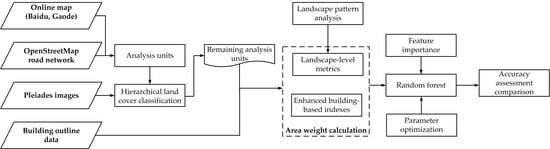
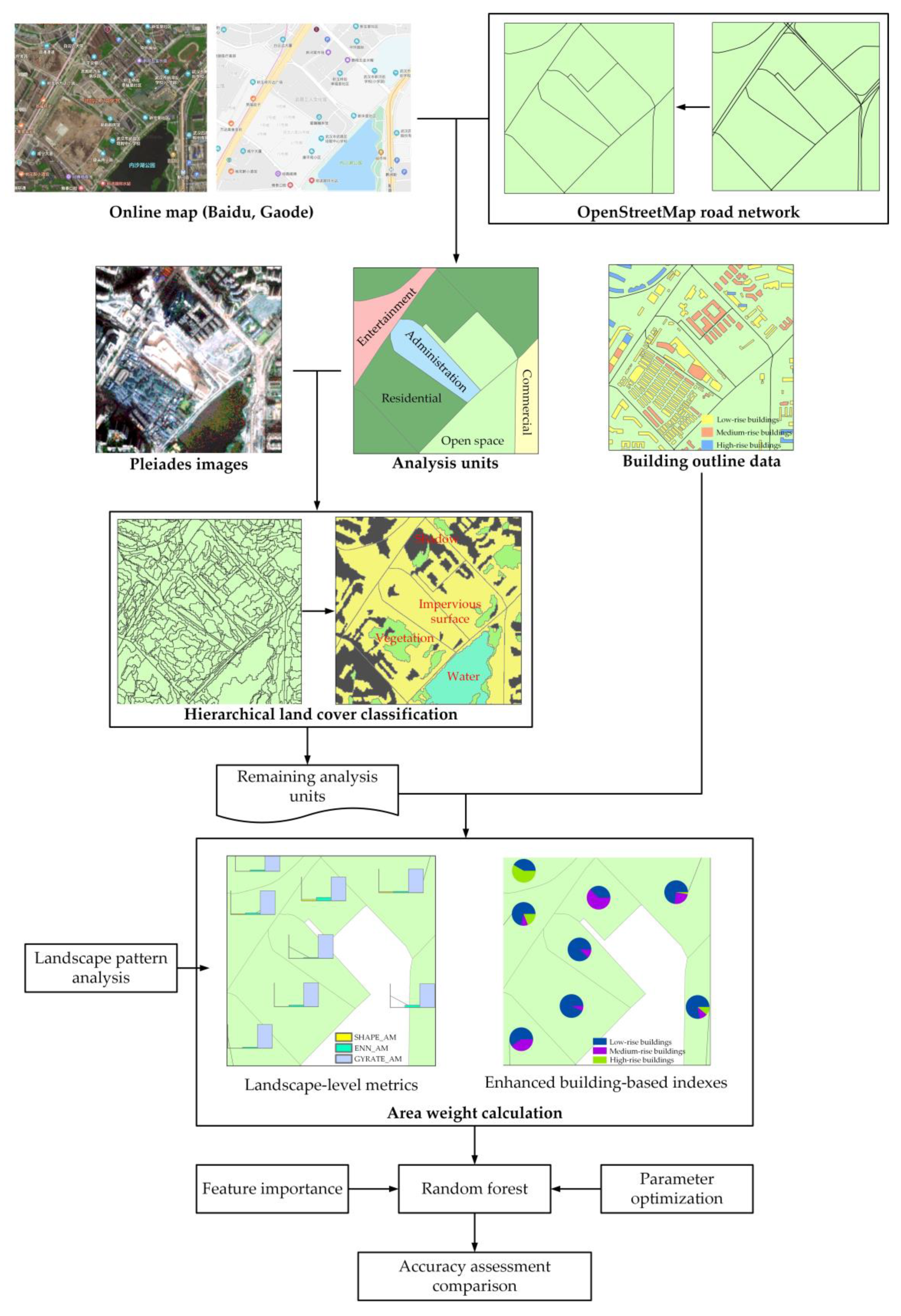
• Inspired by the idea that larger ground objects contribute in greater amounts to urban areas, this research proposed a hierarchical conceptual framework to combine landscape patterns and building functions for urban land-use classification.
• Multiple area-weighted mean landscape-level metrics to describe landscape patterns were selected.
• Various impervious surface area-weighted building-based indexes to identify building functions were proposed.

As summarized earlier, mean landscape metrics and mean building-based indexes showed their potential in urban land use. This paper moves forward by taking the area weights of different types of ground objects into consideration. Its goal is to map urban areas based on the analysis units and adopt a general approach by exploring multifaceted information (1) extracting various physical features to classify urban land cover, and (2) using landscape-level metrics and building-based indexes to provide socioeconomic attributes to classify urban land use.

The remainder of this paper is organized as follows: Section 2 describes the details of the study area and multiple data. Section 3 introduces the methods for feature extraction and urban land-cover/land-use classification. Section 4 provides a further discussion of the obtained results. Finally, conclusions are stated in Section 5.

2. Materials and Methods

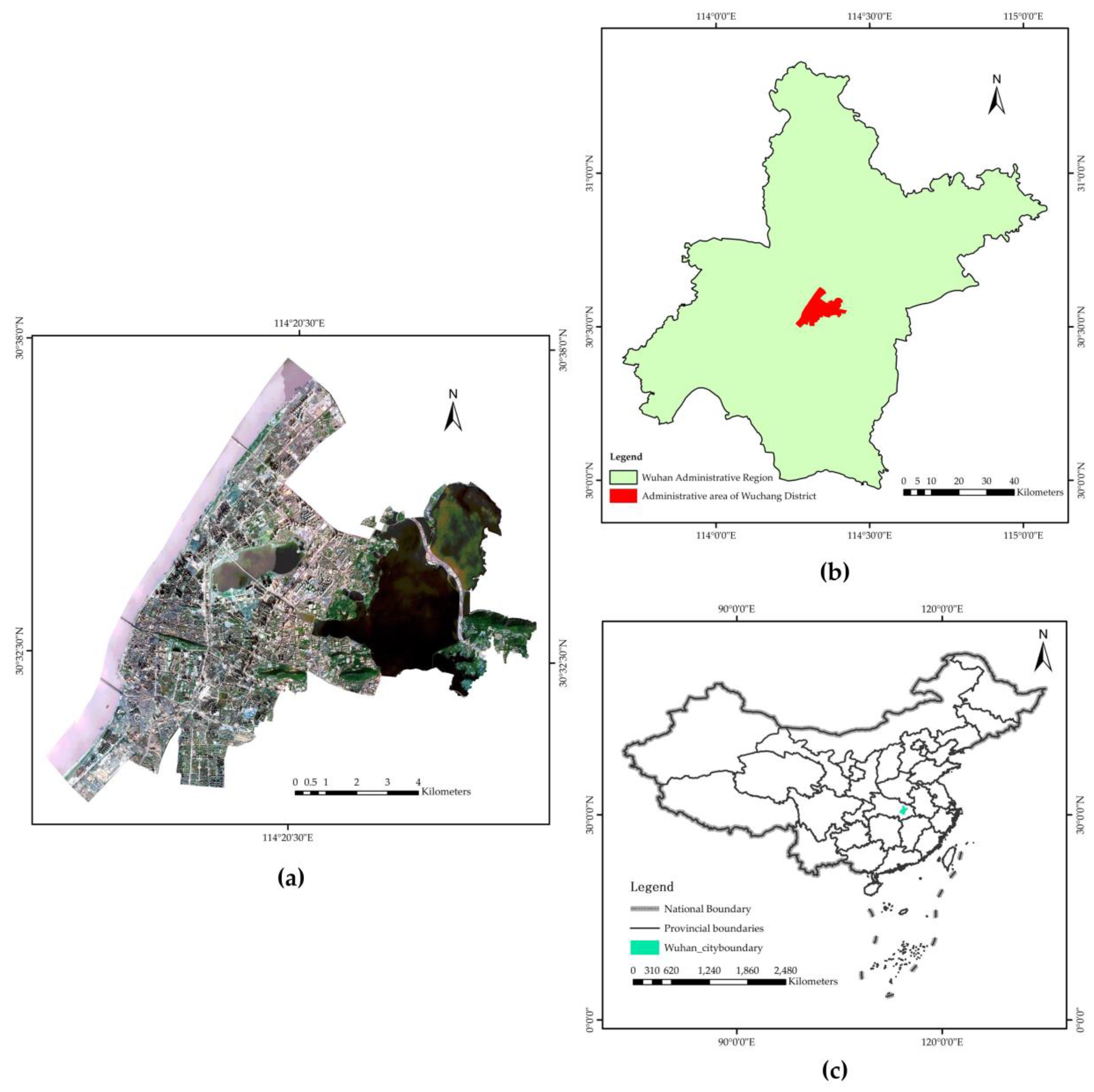
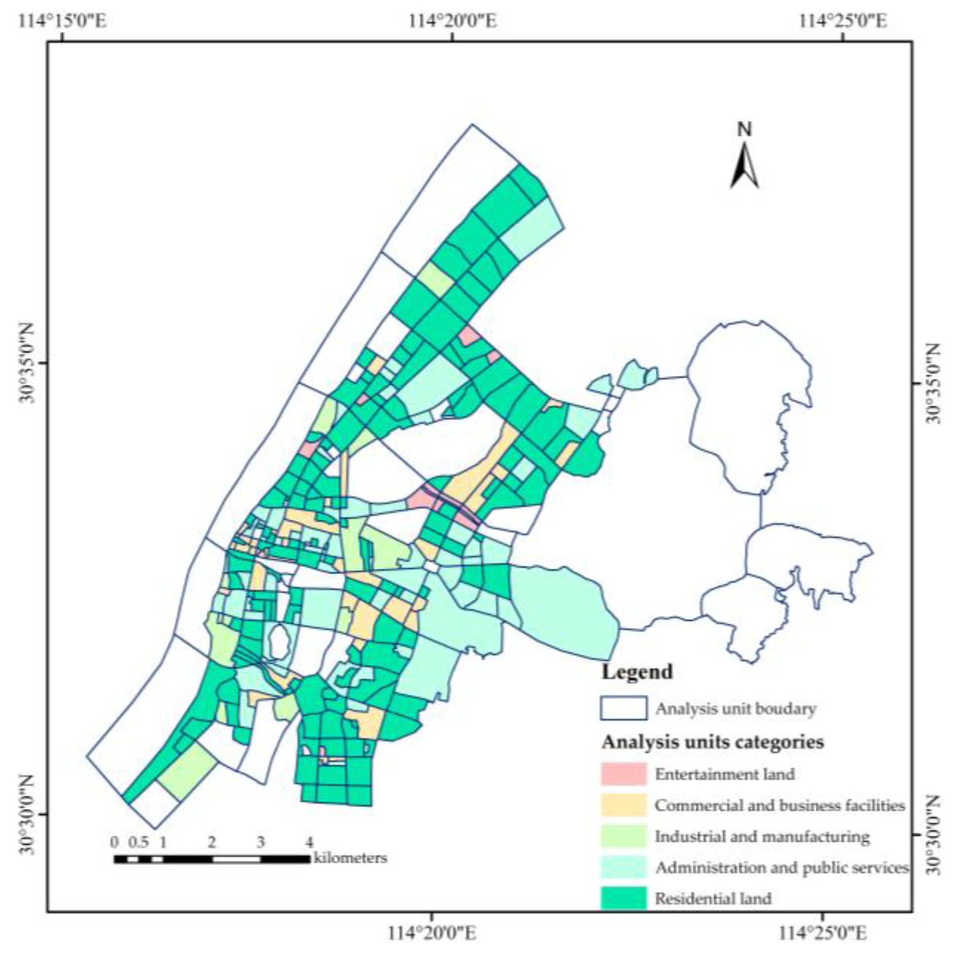
2.1. Study Area

The study area (described in Figure 1), Wuchang District, is one of the main districts of Wuhan city, Hubei Province. The total municipal administrative area of Wuchang District is 64.58 km², with a permanent population of 1.26 million in 2014. In this area, various typical ground object types exist—large amounts of highly intensive buildings, plentiful vegetation, and a multitude of water resources, generating a highly heterogeneous landscape pattern. Moreover, Wuchang is not only the seat of the provincial government department, but also the political, educational, and industrial center. It has diversified types of urban land use, such as administration and public services, industrial and manufacturing, and commercial services. Hence, it is meaningful to depict the current land use of Wuchang District.

2.2. Data and Preprocessing

This work exploited various information extracted from high-spatial-resolution remote sensing images and building outline data to classify urban land use. The following parts of this section describe the separate usage of the three data sources. All the datasets were geometrically corrected and referenced to the UTM WGS84 coordinate system.

2.2.1. High-Spatial-Resolution Remote Sensing Image and Preprocessing

The primary high-spatial-resolution remote sensing image was from the Pleiades 1A satellite sensor from Airbus Defense and Space, which was launched in December 2011. It provides a panchromatic channel with 0.5-m resolution and four spectral bands (blue, green, red, and near-infrared) with a 2-m resolution. Furthermore, it revisits any point on Earth daily, and the swath width is over 20 km at nadir. The image was acquired on 21 January 2015. Thus, the green band must be enhanced to illustrate the surface vegetation more clearly. The image enhancement was implemented in the software ENVI in three steps. Firstly, the Normalized Difference Vegetation Index (NDVI) tool was used to transform multispectral data into a single band. Secondly, the Band Math tool was used to apply a mathematical operation or interactive data language (IDL) function for building the new green band. The expression is defined as follows:

$$(\mathrm{NDVI}\mathrm{gt}0.2)\times (\mathrm{GREEN}\times 0.8+\mathrm{NIR}\times 0.2)+(\mathrm{NDVI}\mathrm{le}0.2)\times \mathrm{GREEN}$$

(1)

where gt is an IDL syntax which means “greater than”, NIR refers to the original near red band, and le is an IDL syntax which means “less than or equal to”.

Thirdly, the Build Layer Stack tool was used to build a true color (RGB) image from the original red band, the new green band, and the original blue band.

In addition, different types of buildings have different exterior surfaces and a considerable portion of the buildings are hard to discern from roads based on physical features. Therefore, without impacting the land-use classification, buildings and roads in this paper were classified together as impervious surface.

2.2.2. Building Outline Data and Preprocessing

The building outline data were acquired in about 2018 provided by Gaode (https://www.amap.com/). Gaode Maps is created by AutoNavi Software Company, which is one of the largest map providers in China and leads the navigation market in the past few years [32,33]. Each item contains information about the identifier (ID), floor, and perimeter of a single building. The topology of the data was validated and modified in the software ArcMap 10.5.

A group of buildings can be defined based on the national standard, previous studies, or the actual situation. For example, according to the Chinese national standard of general rule for architectural design of civil buildings (GB50352-2019), this work took the building height as the criterion to divide the buildings into three broad groups. Regarding the actual situation, this work subdivided the building into four groups: low-rise buildings (1–3 floors), medium-rise buildings (4–10 floors), high-rise buildings (11–40 floors), and super high-rise buildings (>40 floors). The stacked bar chart in Figure 2 displays the percentage of the number of different building groups in each analysis unit. In a bar, each color corresponds to one of the four building groups and the color bar length represents the percentage of the number of the corresponding building group in the analysis unit. As we can see, most analysis units have a larger percentage of the low-rise buildings than other building groups. Compared with other building groups, this will make the number and area information from the low-rise buildings hold more weight in the urban land use classification.

2.2.3. OpenStreetMap Road Network and Preprocessing

OSM collects data from volunteers with the help of manual surveys, global position system instruments, and other free services. Its availability in urban land-use classification was proven in [20]. This research used a semiautomated method to develop the OSM road network to create the fundamental analysis units for mapping urban areas.

2.3. Methodology

The workflow of the proposed method is depicted in Figure 3. It comprises three parts: constructing analysis units, mapping urban land cover, and classifying urban land use. Based on the generated analysis units, the remote sensing image of the study area was divided into image tiles. Within each image tile, a four-level hierarchical method was adopted to classify the preprocessed remote sensing image into vegetation, shadow, water bodies, soil, and impervious surfaces. Following this, waters and open space were preliminarily identified from all analysis units. After the preliminary classification, the remaining analysis units were categorized by analyzing landscape patterns and building functions.

2.3.1. Analysis Unit Construction

Urban blocks are defined as the space delineated by the road network. Compared with uniform rectangular grids [34], their clear boundaries present conceptual accuracy, making it closer to a realistic cognition. This work improved the analysis units by using the OSM road network with the support of other online maps. The usage of freely accessible OSM data increased the transferability of the approved approach. The details are as follows:

• The preliminary road network of Wuchang District was constructed from the OSM data, and the road central line of the raw OSM road network was extracted in the ArcMap.
• After modifying the topology in the ArcMap 10.5, the second step was to remove the dangling roads and update the road network to form road segments.
• This paper constructed the 305 analysis units through the visual interpretation of online maps, such as Baidu Maps and Gaode Maps, and the a priori knowledge of local people [24,35]. In addition, each of them was annotated for one dominant land-use type (the type standards are discussed in Section 2.3.4) [36]. Consequently, this can also be used as the reference data for validation in the following experiments.

2.3.2. Hierarchical Land-Cover Mapping

The spectrum, texture, size, and shape of ground objects vary greatly. In this part, multiple physical features were extracted to explore land-cover information. As opposed to the pixel-based classification method, the geospatial object-based image classification paradigm has four main components: (1) the segmentation procedure, (2) the hierarchy classification method, (3) the integration of expert knowledge, and (4) the feature space optimization [37]. In order to process the remote sensing data conveniently and quickly, the procedures of image segmentation [38], feature extraction [27], and feature space optimization were all completed using the eCognition software. Firstly, constrained by the assigned analysis units, this paper combined the multiresolution segmentation method (MRIS) and the spectral difference segmentation method (SDA) to divide each image tile into segments.

MRIS is a widely used bottom-up segmentation algorithm [10], which aims at minimizing the average heterogeneity and maximizing the respective homogeneity. More specifically, this homogeneity is defined as a combination of spectral homogeneity and shape homogeneity [39]. The scale parameter, which stipulates the maximum allowable heterogeneity for the image objects, was set to 20. The shape parameter, which defines the textual homogeneity of the resulting objects, was set to 0.5. The compactness parameter, which adjusts the degree of compactness to optimize the resulting objects, was set to 0.5. SDA merges neighboring, spectrally similar image objects [39] and refines the existing segmentation result from the MRIS-based segmentation. The scale parameter, which stipulates the maximum allowed heterogeneity for the image objects, was set to 5. Finally, the image was segmented into 400,925 objects. Multiple physical features (

Table 1. Physical characteristics of the high-spatial-resolution remote sensing image. NIR—near-infrared.

Category	Name	Description
Customized Indices	Normalized difference vegetation index (NDVI) [40]	$\mathrm{NDVI}=\frac{\mathrm{NIR}-\mathrm{RED}}{\mathrm{NIR}+\mathrm{RED}}$
	Normalized difference water index (NDWI) [41]	$\mathrm{NDWI}=\frac{\mathrm{GREEN}-\mathrm{NIR}}{\mathrm{NIR}+\mathrm{GREEN}}$
	Soil-adjusted vegetation index (SAVI) [42]	$\mathrm{SAVI}=\frac{(1+\mathrm{L})(\mathrm{NIR}-\mathrm{RED})}{\mathrm{NIR}+\mathrm{RED}+\mathrm{L}}$
	Shadow index (SI)	SI = |RED + GREEN − 2BLUE|
Texture	Gray-level co-occurrence matrix (GLCM) mean, GLCM entropy, GLCM contrast, GLCM correlation, GLCM dissimilarity [43]
Spectrum	Mean blue, mean green, mean red, mean NIR, mean brightness
	Standard deviation blue, standard deviation green, standard deviation red, standard deviation NIR
	Skewness blue, skewness green, skewness red, skewness NIR
Geometry	Area
	Length/width
	Border index
	Compactness
	Elliptic fit
	Rectangular fit
	Roundness
	Shape index

) of image objects were extracted for the land-cover classification.

According to the practical experiment, this work made some modifications to the hierarchical classification method. During the hierarchical land-cover classification, the vegetation was firstly extracted from the NDVI image. A membership function was used to define the relationship between the NDVI values and the degree of membership to vegetation using fuzzy logic [44]. High values of NDVI correspond to vegetation. It was assumed that image objects with values above 0.12 corresponded to the “vegetation” class, and low values of NDVI (0.087 and below) represented the “non-vegetation” class. From 0.12 to 0.087, as the fuzzy membership decreased, the possibility of “non-vegetation” increased. Secondly, the shadow was separated using shadow index (SI) and area. The thresholds were set to 200 and 125,000, respectively. That is to say, the image object whose SI value was less than 200 and whose area value was less than 125,000 was assigned to the “shadow” class. Thirdly, water bodies were extracted by soil-adjusted vegetation index (SAVI) and area. Although the Normalized difference water index (NDWI) was originally designed to extract water bodies, when extracting water bodies in the city, the building shadow can seriously interfere with the NDWI. Due to the high sediment concentration, this work tested SAVI to extract water bodies and obtained a reasonable result. The image objects whose SAVI values were less than 0.04 and whose area values were greater than 100,000 were assigned to the “water” class. Compared with NDVI, SAVI adds a constant, L, to reduce the soil background effect. Generally, the adjustment factor L = 0.5 was used to minimize the soil variations.

After extracting the features, a ranking of features or feature combinations in order of significance is typically provided. Differing from References [32,41], the physical features extracted above were optimized in eCognition using a standard function—feature space optimization to select the best combination of features for convenience. The goal was to select the best combination of features corresponding to the largest average minimum distance between the samples of different classes. The best separation distance was 1.165. Based on the other features, all the remaining segmented objects were classified using the support vector machine classifier. This work revised the training samples according to the accuracy assessment results.

2.3.3. Preliminary Classification

Land-cover classification essentially emphasizes the physical and biological objects of an area, like grassland, water, or bare rock. On the other hand, land-use classification is concerned with the socioeconomic functions, such as the residential land or entertainment land [37,45]. Land-cover classification results are widely used as the landscape elements to measure landscape patters for land use classification [1,18,20,24]. Since the shadow in the remote sensing image of the study area is too large to ignore, it was classified as one of the land-cover classification categories. However, it should not be considered as a landscape element. We removed the shadow from the land-cover map and calculated the landscape metrics of other areas.

Moreover, different proportions of water bodies and vegetation are significant for classifying analysis unit types to some extent, in particular for preliminarily identifying the waters and open space. Repeated experiments indicated that the analysis units where the vegetation was scarce and water body coverage was greater than 60% should be identified as waters. Parks were the analysis units with water bodies covering more than 50% area and where the sum of the proportion of water bodies and vegetation was greater than 60%. The other open spaces, like green lands or squares, were the analysis units where the vegetation coverage area exceeded 50%. The work below analyzes the landscape patterns and building-based information of the remaining 269 analysis units for further land-use classification.

With regard to the remaining analysis units, there is no standard and consistent type of urban land use. The standard of urban land-use categories is different due to the different study areas and research objectives [45]. The latest Chinese standard of current land-use classification (GB/T 21010-2017) classifies development land into eight categories. According to the actual situation of Wuchang District, the development land falls into five categories, excluding waters and open space: (a) commercial and business facilities; (b) administration and public services; (c) industrial and manufacturing; (d) residential land; (e) entertainment land.

To better understand the impact of spatial arrangements and compositions of landscape elements on the type of landscape mosaic (that is, analysis unit types), Figure 4 schematically illustrates the relationship between urban landscape structures and the corresponding type of analysis units. As shown in Figure 4, compared with other types of areas, the spatial distribution of shadows in the residential land is evenly distributed, and the number and height of buildings are relatively large and short, respectively. Apart from the impervious surfaces, other ground object categories in residential lands are also more proportional.

2.3.4. Landscape-Level Metrics

Landscape patterns are the concrete embodiment of landscape heterogeneity and are widely used in describing the spatial distribution and configuration of elements within the landscape mosaic. Landscape metrics are defined at the patch level, class level, or landscape level. Selecting landscape metrics can be based on expert knowledge, previous studies, and the theoretical explanation of indexes [46]. In terms of the aspect of landscape pattern measured, the landscape metrics are grouped as follows: area and edge metrics, shape metrics, contrast metrics, aggregation metrics, and diversity metrics [47]. Among them, the shape metric is crucial in describing the urban landscape [1,47,48]. In summary, depending on the landscape context, this work selected the following groups of landscape metrics: area and edge metrics, shape metrics, aggregation metrics, and diversity metrics. Based on the analysis units, nine landscape-level metrics were calculated (

Table 2. The selected landscape metrics in the urban land-use classification.

Aspect of Landscape Pattern	Landscape Metric	Abbreviation
Area and edge metrics	Area-weighted mean patch radius of gyration index	GYRATE_AM
Shape metrics	Area-weighted mean patch perimeter–area ratio index	PARA_AM
	Area-weighted mean patch shape index	SHAPE_AM
	Area-weighted mean patch fractal dimension index	FRAC_AM
	Area-weighted mean patch related circumscribing circle index	CIRCLE_AM
	Area-weighted mean patch contiguity index	CONTIG_AM
Aggregation metrics	Area-weighted mean patch Euclidean nearest neighbor distance index	ENN_AM
Diversity metrics	Shannon’s diversity index	SHDI
	Modified Simpson’s diversity index	MSIDI

) in Fragstats 4.2 software to measure landscape pattern for urban land-use classification.

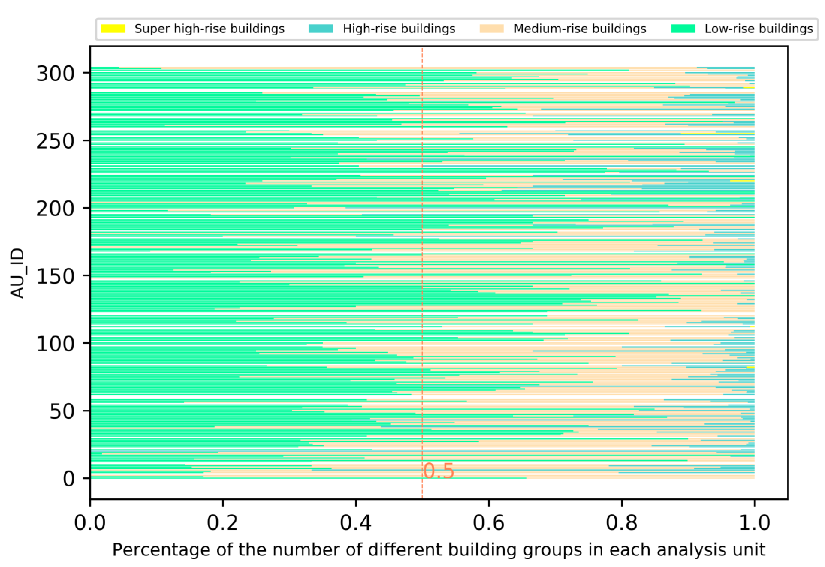
2.3.5. Enhanced Building-Based Indexes

Building-based information is essential to identify building functions for classifying analysis units. It is widely proven that building number and building area can effectively indicate building functions [3,28,29]. However, previous researchers generally used mean building number index and mean building area index, regardless of the fact that the impervious surface area, where all the buildings are located, is dominant in urban areas. This work improved the common building-based indexes by multiplying the ratio of the impervious surface area within each analysis unit to the impervious surface area of the entire study area and using the building height as the grouping criterion.

Table 3. Mathematical details of the enhanced building-based indexes.

Building-Based Index		Abbr.	Formula
Impervious area-weighted building number index	Impervious surface area-weighted low-rise building number index	BN_IA1	${\left(\mathrm{BN}\_{\mathrm{IA}}_i\right)}_j={\mathrm{n}}_{\mathrm{ij}}\times \frac{{\mathrm{a}}_{\mathrm{i}}}{\mathrm{A}}$
	Impervious surface area-weighted medium-rise building number index	BN_IA2
	Impervious surface area-weighted high-rise building number index	BN_IA3
	Impervious surface area-weighted super high-rise building number index	BN_IA4
	Impervious surface area-weighted sum building number index	BN_IA_SUM	${(\mathrm{BN}\_\mathrm{IA}\_\mathrm{SUM})}_{\mathrm{j}}={\left({\displaystyle {\displaystyle \sum }_{\mathrm{i}}}{(\mathrm{BN}\_\mathrm{IA}}_{\mathrm{i}})\right)}_{\mathrm{j}}$
Impervious area-weighted building area index	Impervious surface area-weighted low-rise building area index	BA_IA1	${\left(\mathrm{BA}\_{\mathrm{IA}}_i\right)}_j={\mathrm{a}}_{\mathrm{ij}}\times \frac{{\mathrm{a}}_{\mathrm{i}}}{\mathrm{A}}$
	Impervious surface area-weighted medium-rise building area index	BA_IA2
	Impervious surface area-weighted high-rise building area index	BA_IA3
	Impervious surface area-weighted super high-rise building area index	BA_IA4
	Impervious surface area-weighted sum building area index	BA_IA_SUM	${(\mathrm{BA}\_\mathrm{IA}\_\mathrm{SUM})}_{\mathrm{j}}={\left({\displaystyle {\displaystyle \sum }_{\mathrm{i}}}{(\mathrm{BA}\_\mathrm{IA}}_{\mathrm{i}})\right)}_{\mathrm{j}}$

Note: i: the serial number of building group; j: the serial number of analysis unit; a_i: impervious surface area (m²) of analysis unit j; A: total impervious surface area (m²); n_ij: the number of building grouping i of analysis unit j; a_ij: the area of building grouping i of analysis unit j.

illustrates the enhanced building-based indexes corresponding to the four building groups.

2.3.6. Random Forest

Considering the different value ranges of various landscape-level metrics and building-based indexes, this work adopted random forest to combine features as widely applied [27,49]. Huang et al. classified building types based on light detection and ranging (LiDAR) data and high-spatial-resolution remote sensing images using the random forest classifier [50]. Du et al. used an improved random forest classifier to combine high-resolution remote sensing images and building edge data for classifying buildings semantically [27]. The random forest model is relatively insensitive to feature scales and is able to generate feature importance [24]. Here, the random forest model was from the Scikit-learn Machine Learning Library (scikit-learn.org/stable/) for Python. It combines trees by averaging the probabilistic prediction rather than letting each tree vote for a single class. Among the remaining analysis units, 90% of the units were randomly selected as the training samples, and the others were treated as the testing samples.

To reduce the influence of imbalanced samples, the parameter named class_weight was set to “balanced”. This achieves the goal by automatically adjusting the weights inversely proportional to the class frequencies in the input data. During the model training, two finely tuned parameters were required: n_estimators and max_features. The former denotes the number of trees in the forest. The latter is the number of features to consider when splitting a node. A grid search strategy was used to calibrate the parameters. In this paper, n_estimators was set to 50 and max_features = sqrt(n_features), where n_features is the number of features in the model.

3. Results

In this work, urban area mapping consisted of two processes: urban land-cover classification and urban land use classification. The distinction between them is that the former emphasizes the natural environment, while the latter pays close attention to human activities [51]. The paper analyzed landscape patterns and building functions to represent socioeconomic information for improving urban land use classification. The results and discussion are presented below.

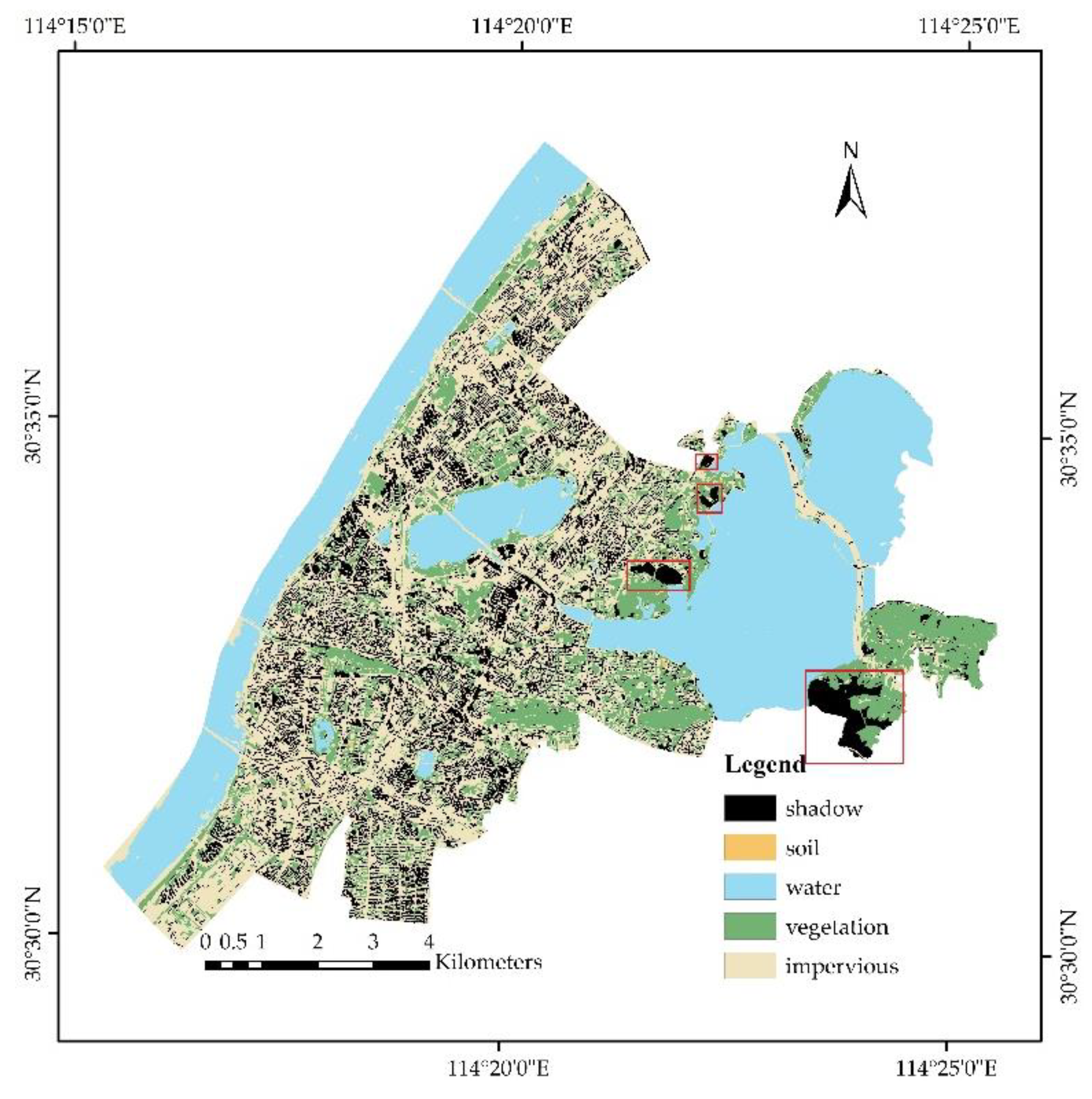
3.1. Land-Cover Classification Results

The land-cover classification results are depicted in Figure 5, which shows that the impervious surface area and shadow of buildings cover most of the study area. Therefore, it can be inferred from the actual situation that identifying building functions is conducive to urban land-use classification. There are several obvious errors where water bodies are misclassified as shadows (marked in red box of Figure 5). It is reasonable to speculate that the high impurity content can result in water having similar spectral and textural characteristics to shadow—both dark and smooth. Fortunately, the analysis units of waters and open space were firstly identified; thus, there is not a large impact on the classification of the remaining analysis units.

According to

Table 4. Confusion matrix of the land-cover classification results.

User Class/ Sample	Shadow	Soil	Water	Vegetation	Impervious Surface	User’s Accuracy
Shadow	1864	0	5	114	77	90.49%
Soil	0	3	0	0	0	1
Water	5	0	36	3	0	81.82%
Vegetation	69	1	0	1220	64	90.10%
Impervious surface	64	7	0	71	4962	97.22%
Producer’s accuracy	93.11%	27.27%	87.80%	86.65%	97.24%	OA = 94.40%
KIA Per Class	90.92%	27.25%	87.74%	84.14%	93.16%	KIA = 90.04%

Note: OA: overall accuracy; KIA: Kappa Index of Agreement.

, the confusion matrix with kappa analysis indicated that the overall accuracy (OA) of the land-cover classification result was 94.40% and the producer’s accuracy of all classes was over 86%, except for the soil class. It is important to highlight that the impervious surface was classified with producer’s accuracy and user’s accuracy over 95% and 93.16% in kappa per class, providing a solid foundation for the subsequent land-use classification.

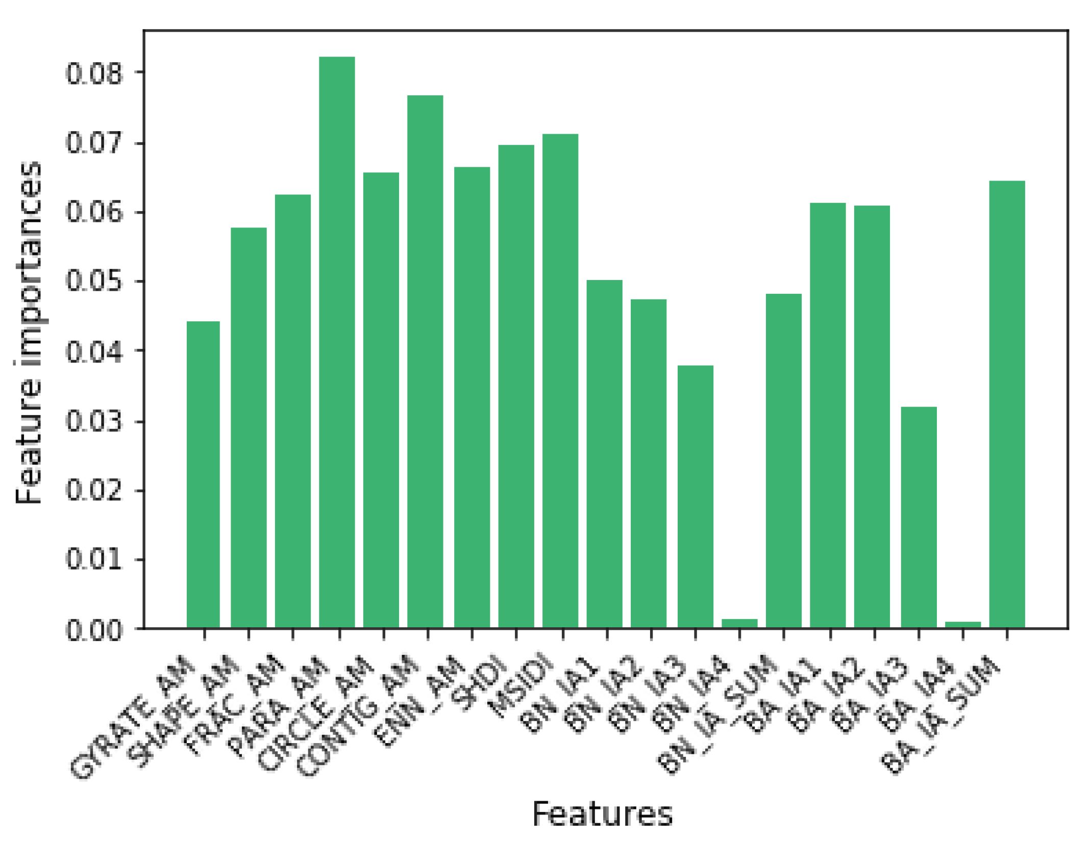
3.2. Evaluation of Feature Importance

It is widely proven that features do not contribute equally to predicting targets [27]. The evaluation of the importance of nine landscape-level metrics and 10 building–based indexes was inspired by a basic idea, i.e., the frequency that a feature is used in the split points of a decision tree reflects the degree of its importance [52]. The feature importance scores were accessed from the attribute named “feature_importances_” in the fitted random forest classifier.

Figure 6 displays the average importance scores of features in the random forest model. It shows that area-weighted mean patch perimeter-area ratio index (PARA_AM), area-weighted mean patch related circumscribing circle index (CONTIG_AM), and modified Simpson’s diversity index (MSIDI) are the top three important features in urban land-use classification. PARA_AM measures landscape configuration in terms of the shape complexity and it varies with the size of the landscape element. Although CONTIG_AM also assesses the shape complexity [53], it convolves a 3 × 3 pixel template with a binary image where the values of pixels are assigned according to the spatial connectedness. MSIDI [54] quantifies the diversity of the landscape based on the modification of Simpson’s diversity index. This feature is proportional to the number of different element types within each landscape mosaic. As already pointed out, different types of landscape mosaics express different spatial compositions and spatial configurations of landscape elements.

The two least significant features, impervious surface area-weighted super high-rise building number index (BN_IA4) and impervious surface area-weighted super high-rise building area index (BA_IA4), measured the number and area of super high-rise buildings, respectively, which is mainly due to the small sample size of super high-rise buildings. This seems to be one reflection of ground objects with larger coverage making a greater contribution to urban area mapping. In conclusion, the proposed urban land-use classification strategy worked reasonably well by considering the area weight.

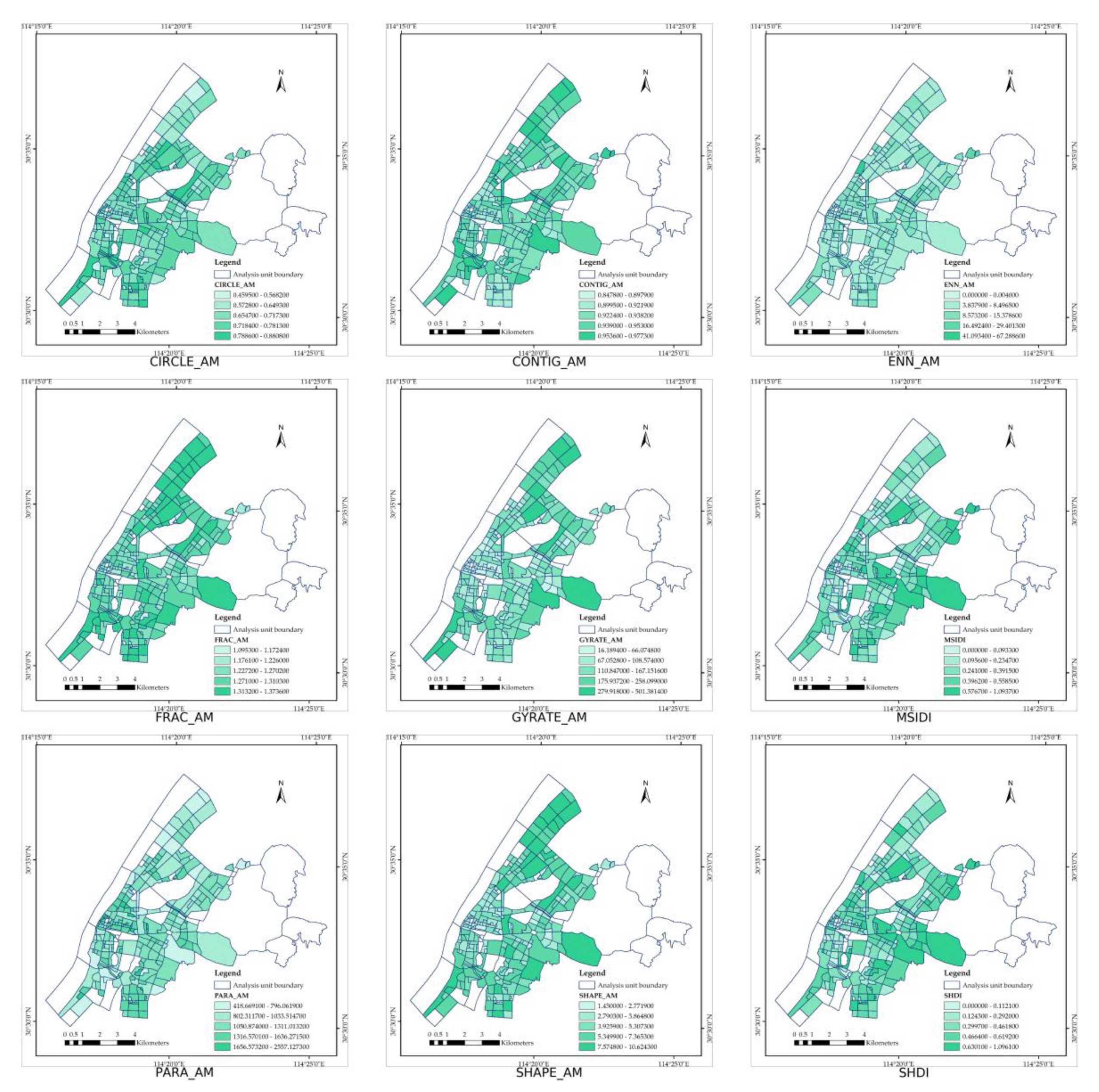
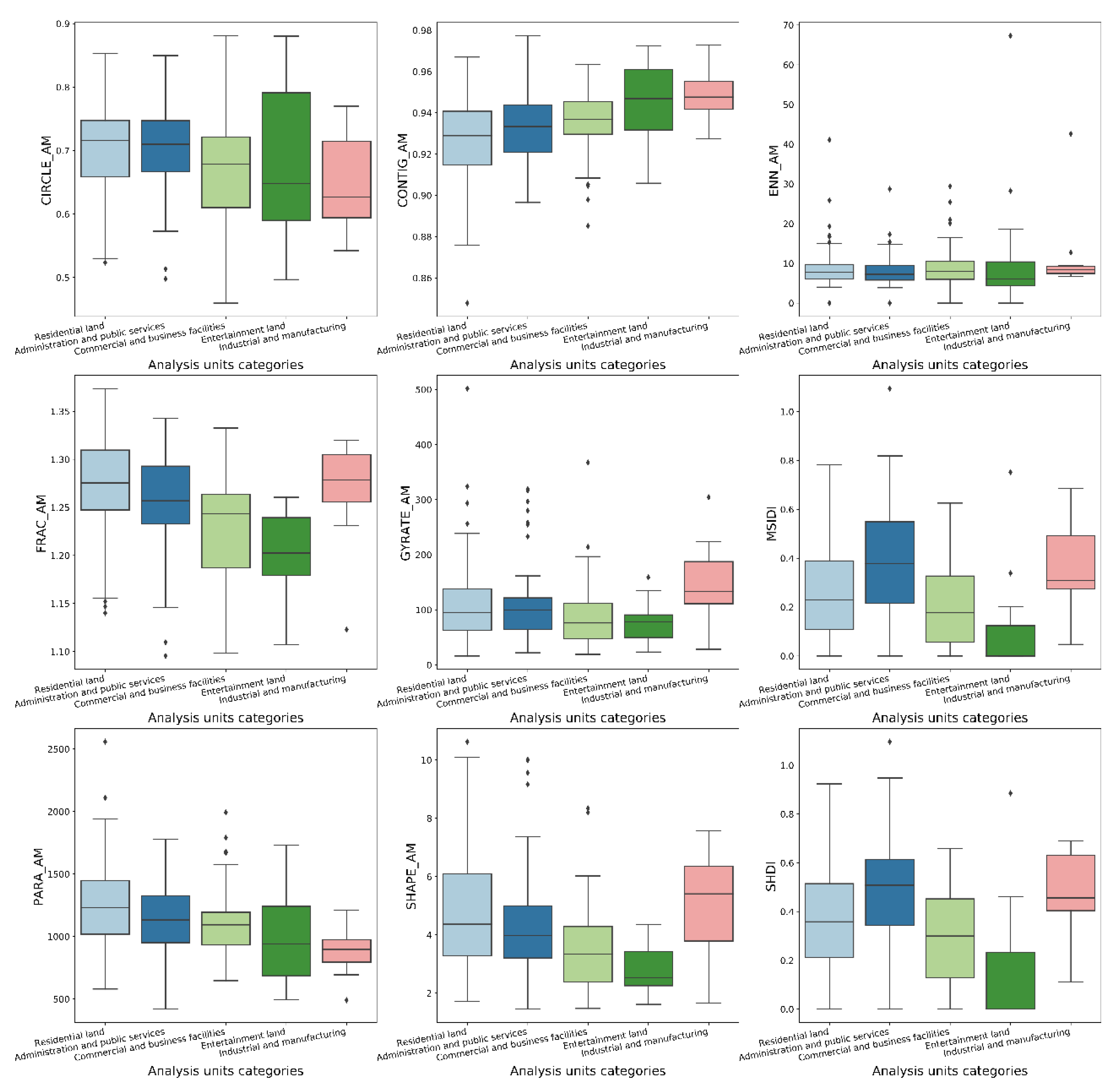
3.3. Landscape Pattern Analysis

Landscape pattern is not only a definite reflection of the landscape heterogeneity, but also the product of the interaction between human activities and the physical geographic environment. Landscape pattern refers to the spatial arrangement and combination form of landscape elements in different sizes and shapes.

From visual interpretation, the landscape pattern indexes of the same land-use type of analysis units stayed in a similar numerical range. The point to emphasize here is that the impervious surface was used to denote buildings and roads. This led to some significant differences in measuring landscape patterns for describing the type of analysis units from previous studies [29,49]. Figure 7, in connection with Figure 9, shows that the five types of analysis units expressed different properties in the four aspects of landscape patterns. Taking the case of residential land, the high radius of gyration shows that the extensiveness of ground objects is high, the high CONTIG_AM represents that the shape of ground objects is irregular and complex, the low area-weighted mean patch Euclidean nearest neighbor distance index (ENN_AM) represents that ground objects of the same type are far apart, and the high Shannon’s diversity index (SHDI) and MSIDI indicate that the distribution ratio of ground object types is less equitable.

The boxplots of the landscape metrics calculated from various types of analysis units are described in Figure 8. In a boxplot, the central line represents the median, and the top and bottom edges are the 75th and 25th percentiles, respectively. The outliers are drawn using the “♦” symbol. As depicted in Figure 8, there are some obvious differences between the landscape patterns of each type of analysis units. For example, compared with the entertainment land, the industrial and manufacturing land had a higher SHAPE_AM and a similar CONTIG_AM. As known to all, SHAPE_AM and CONTIG_AM both describe the shape complexity of analysis units. The subtle difference between them is that SHAPE_AM directly calculates the perimeter–area ratio index of the ground object type, while CONTIG_AM evaluates the shape complexity to the spatial connectedness.

Figure 5, in conjunction with Figure 9, shows that, in comparison with the entertainment land, the industrial and manufacturing land consisted of fewer types of ground objects, as well as larger impervious surface with scattered vegetation. This means they are irregular in arrangement and have poor connectivity, which is consistent with the results. Furthermore, taking MSIDI as an illustration, although there were fewer types of ground objects in the industrial and manufacturing land, their proportions were unevenly distributed. It is acceptable that the MSIDI value of the industrial land was higher than that of the entertainment land. Therefore, the delineated landscape metrics were able to effectively measure landscape pattern for urban land-use classification.

3.4. Land-Use Classification Results

Compared with mapping urban land cover, it is harder to map urban land use due to the complex urban landscape heterogeneity. Analysis units of waters and open space were identified earlier. There were still 269 analysis units. The spatial distribution of the remaining analysis units is illustrated in Figure 9, which exposes the problem of imbalanced sample sizes of analysis units. For instance, a large quantity of residential land covers most of the study area, while entertainment land covers the smallest area. As mentioned before, we alleviated this issue by setting the class_weight to “balanced”.

To quantify the effectiveness of the proposed method, this research compared it with the random forest model, using corresponding mean landscape-level metrics and mean building-based indexes, including GYRATE_MN, PARA_MN, SHAPE_MN, area-weighted mean patch fractal dimension index (FRAC_MN), area-weighted mean patch related circumscribing circle index (CIRCLE_MN), CONTIG_MN, ENN_MN, SHDI, MSIDI, mean building area, and mean building number. These mean characteristics are commonly used to delineate urban land use by urban morphology or building functions [24,28,29]. Due to the actual problems with the sample size, the overall results appear to be low (

Table 5. Classification accuracy results of the compared method.

Method	Precision	F1-Score	Recall
The proposed method	81.26%	76.91%	77.78%
The corresponding mean method 1	70.59%	63.98%	66.67%

¹ The SHPE_MN, ENN_MN, and CONTIG_MN used in Reference [24]. The mean building area, mean building number, and FRAC_MN used in Reference [29]. The GYRATE_MN, PARA_MN, CIRCLE_MN, and MSIDI computed in Reference [47].

). However, compared with the common method, the precision increased by 10.67%, the F1-score increased by 12.93%, and the recall score increased by 11.11%.

4. Discussion

Improving urban land-use classification accuracy is an urgent problem in the field of urban study, such as urban structure and urban dynamics analysis. As shown in Table 5, the proposed method achieved appreciable improvement in the precision, the F1-score, and the recall score. This demonstrated that the area weights of different types of ground objects vary in urban area mapping, and it helps to improve the classification accuracy. Overall, the impact of landscape patterns on urban land use is greater than building functions. In terms of the four building groups, the number of each group determines the ranking of the feature extracted from them. Compared with other similar studies, this study found that a larger size of ground objects resulted in a greater impact on the urban land-use classification.

The proposed method in this study used various features derived from high-spatial-resolution remote sensing images, building outline data, and OSM road networks to map urban areas. The analysis units were constructed based on the OSM road network. Both the OSM road network and the building outline data can be crawled on the internet. Therefore, if similar high-spatial-resolution images (e.g., QuickBird, GeoEYE, and WorldView-2) are available in other places, the presented approach is applicable without any modification.

There are some limitations of the study. Firstly, the shadow in the remote sensing image covers large areas. It leaves many unknown areas and loses the relevant landscape patterns used for land-use classification. Secondly, the land-use classification relies much on the early GEOBIA, which requires a lot of effort to obtain a satisfactory result. However, this is just workload, not innovation. Thirdly, compared with social sensing data, remote sensing data and building outline data offer less socioeconomic information of urban areas, which will be accomplished in future.

5. Conclusions

Measuring the landscape pattern and inferring building functions provides a useful idea for urban land-use classification. Based on the analysis units, this study provided a random forest model-based framework that combined landscape-level metrics and building-based indexes for urban land-use classification. This work implemented urban area mapping in multiple steps. Firstly, within each unit, various physical features of the segmented objects were extracted from remote sensing images to hierarchically classify the urban land cover. Secondly, based on the land-cover map, the landscape patterns of different types of analysis units were analyzed. Meanwhile, the enhanced building-based indexes were computed from the building outline data. Lastly, the random forest model was conducted with landscape-level metrics and building-based indexes for urban land-use classification. The results showed the applicability and effectiveness of the proposed method. Specifically, the F1-score increased by 8.42% and the recall score increased by 11.11%. Therefore, it provides a useful tool to describe urban areas. It helps decision-makers understand the current urban land use and spatial structure for future urban planning and sustainable development.

The existing literature treats various types of ground objects with equal importance in each analysis unit. However, different types and sizes of ground objects contribute differently to land-use categories. Specifically, the impervious surface plays a significant role in urban areas. In order to abide by reality, this work enhanced the landscape-level metrics and building-based indexes by applying area weights and using building height as the grouping criterion. It is a successful attempt to combine landscape patterns and building functions to explore socioeconomic information in urban areas. By providing a general analysis framework, if similar high-resolution images are available in other cities, the study can be extended to similar studies elsewhere. Moreover, this study contributes to supporting urban planning and development.

In the future, this research will expand to introduce more social sensing data into urban land-use study, such as taxi trajectory data, check-in data, and points of interest (POIs). For instance, taxi trajectory data imply human travel patterns, linking the purpose of travel to urban land use. Furthermore, based on the urban land-use classification result, taxi flows can help measure the interaction between different types of analysis units. Compared with building outline data, POIs provide more accurate and intuitive information about building functions. The density of POIs directly reflects the intensity of land use. Moreover, the distribution of POIs can improve the verification of detailed urban activities related to different land-use types. Social sensing data are able to improve the analysis unit types and infer the spatial interaction between them. More feature fusion methods should be tested in future studies to make more efficient use of multisource features.

References

1. Jiao, L.; Liu, Y.; Li, H. Characterizing land-use classes in remote sensing imagery by shape metrics. ISPRS J. Photogramm. Remote Sens. 2012, 72, 46–55. [Google Scholar] [CrossRef]
2. Tu, Y.; Chen, B.; Zhang, T.; Xu, B. Regional Mapping of Essential Urban Land Use Categories in China: A Segmentation-Based Approach. Remote Sens. 2020, 12, 1058. [Google Scholar] [CrossRef] [Green Version]
3. Beykaei, S.A.; Zhong, M.; Shiravi, S.; Zhang, Y. A hierarchical rule-based land use extraction system using geographic and remotely sensed data: A case study for residential uses. Transp. Res. Part C Emerg. Technol. 2014, 47, 155–167. [Google Scholar] [CrossRef]
4. Zhang, J.; Li, P.; Wang, J. Urban built-Up area extraction from landsat TM/ETM+ images using spectral information and multivariate texture. Remote Sens. 2014, 6, 7339–7359. [Google Scholar] [CrossRef] [Green Version]
5. Lv, Z.Y.; Liu, T.F.; Zhang, P.; Benediktsson, J.A.; Lei, T.; Zhang, X. Novel adaptive histogram trend similarity approach for land cover change detection by using bitemporal very-high-resolution remote sensing images. IEEE Trans. Geosci. Remote Sens. 2019, 57, 9554–9574. [Google Scholar] [CrossRef]
6. Lippitt, C.D.; Zhang, S. The impact of small unmanned airborne platforms on passive optical remote sensing: A conceptual perspective. Int. J. Remote Sens. 2018, 39, 4852–4868. [Google Scholar] [CrossRef]
7. Gong, P.; Howarth, P.J. The use of structural information for improving land-cover classification accuracies at the rural-urban fringe. Photogramm. Eng. Remote Sens. 1990, 56, 67–73. [Google Scholar]
8. Lu, D.; Weng, Q. Use of impervious surface in urban land-use classification. Remote Sens. Environ. 2006, 102, 146–160. [Google Scholar] [CrossRef]
9. D’Oleire-Oltmanns, S.; Coenradie, B.; Kleinschmit, B. An object-based classification approach for mapping migrant housing in the mega-urban area of the Pearl River Delta (China). Remote Sens. 2011, 3, 1710–1723. [Google Scholar] [CrossRef] [Green Version]
10. Blaschke, T. Object based image analysis for remote sensing. ISPRS J. Photogramm. Remote Sens. 2010, 65, 2–16. [Google Scholar] [CrossRef] [Green Version]
11. Lv, Z.; Liu, T.; Benediktsson, J.A. Object-Oriented Key Point Vector Distance for Binary Land Cover Change Detection Using VHR Remote Sensing Images. IEEE Trans. Geosci. Remote Sens. 2020, 1–10. [Google Scholar] [CrossRef]
12. Guo, J.; Zhou, H.; Zhu, C. Cascaded classification of high resolution remote sensing images using multiple contexts. Inf. Sci. (NY) 2013, 221, 84–97. [Google Scholar] [CrossRef]
13. Bratasanu, D.; Nedelcu, I.; Datcu, M. Bridging the Semantic Gap for Satellite Image Annotation and Automatic Mapping Applications. IEEE J. Sel. Top. Appl. Earth Obs. Remote Sens. 2011, 4, 193–204. [Google Scholar] [CrossRef] [Green Version]
14. Zhang, X.; Du, S. A Linear Dirichlet Mixture Model for decomposing scenes: Application to analyzing urban functional zonings. Remote Sens. Environ. 2015, 169, 37–49. [Google Scholar] [CrossRef]
15. Zhang, W.; Li, W.; Zhang, C.; Hanink, D.M.; Li, X.; Wang, W. Parcel-based urban land use classification in megacity using airborne LiDAR, high resolution orthoimagery, and Google Street View. Comput. Environ. Urban Syst. 2017, 64, 215–228. [Google Scholar] [CrossRef] [Green Version]
16. Peng, J.; Wang, Y.; Zhang, Y.; Wu, J.; Li, W.; Li, Y. Evaluating the effectiveness of landscape metrics in quantifying spatial patterns. Ecol. Indic. 2010, 10, 217–223. [Google Scholar] [CrossRef]
17. Stokes, E.C.; Seto, K.C. Characterizing and measuring urban landscapes for sustainability. Environ. Res. Lett. 2019, 14, 045002. [Google Scholar] [CrossRef]
18. Pan, T.; Lu, D.; Zhang, C.; Chen, X.; Shao, H.; Kuang, W.; Chi, W.; Liu, Z.; Du, G.; Cao, L. Urban Land-Cover Dynamics in Arid China Based on High-Resolution Urban Land Mapping Products. Remote Sens. 2017, 9, 730. [Google Scholar] [CrossRef] [Green Version]
19. Voltersen, M.; Berger, C.; Hese, S.; Schmullius, C. Object-based land cover mapping and comprehensive feature calculation for an automated derivation of urban structure types at block level. Remote Sens. Environ. 2014, 154, 192–201. [Google Scholar] [CrossRef]
20. Grippa, T.; Georganos, S.; Zarougui, S.; Bognounou, P.; Diboulo, E.; Forget, Y.; Lennert, M.; Vanhuysse, S.; Mboga, N.; Wolff, E. Mapping urban land use at street block level using OpenStreetMap, remote sensing data, and spatial metrics. ISPRS Int. J. Geoinf. 2018, 7, 246. [Google Scholar] [CrossRef] [Green Version]
21. Edwards, R.; Batty, M. City size: Spatial dynamics as temporal flows. Environ. Plan. A Econ. Space 2015, 48, 1001–1003. [Google Scholar] [CrossRef] [Green Version]
22. Zheng, X.; Wang, Y.; Gan, M.; Zhang, J.; Teng, L.; Wang, K.; Shen, Z.; Zhang, L. Discrimination of settlement and industrial area using landscape metrics in rural region. Remote Sens. 2016, 8, 845. [Google Scholar] [CrossRef] [Green Version]
23. Tu, W.; Hu, Z.; Li, L.; Cao, J.; Jiang, J.; Li, Q.; Li, Q. Portraying urban functional zones by coupling remote sensing imagery and human sensing data. Remote Sens. 2018, 10, 141. [Google Scholar] [CrossRef] [Green Version]
24. Zhang, Y.; Li, Q.; Huang, H.; Wu, W.; Du, X.; Wang, H. The combined use of remote sensing and social sensing data in fine-grained urban land use mapping: A case study in Beijing, China. Remote Sens. 2017, 9, 865. [Google Scholar] [CrossRef] [Green Version]
25. Aguilera, F.; Valenzuela, L.M.; Botequilha-Leitão, A. Landscape metrics in the analysis of urban land use patterns: A case study in a Spanish metropolitan area. Landsc. Urban Plan. 2011, 99, 226–238. [Google Scholar] [CrossRef]
26. Yoshida, H.; Omae, M. An approach for analysis of urban morphology: Methods to derive morphological properties of city blocks by using an urban landscape model and their interpretations. Comput. Environ. Urban Syst. 2005, 29, 223–247. [Google Scholar] [CrossRef]
27. Du, S.; Zhang, F.; Zhang, X. Semantic classification of urban buildings combining VHR image and GIS data: An improved random forest approach. ISPRS J. Photogramm. Remote Sens. 2015, 105, 107–119. [Google Scholar] [CrossRef]
28. Xing, H.; Meng, Y. Measuring urban landscapes for urban function classification using spatial metrics. Ecol. Indic. 2020, 108, 105722. [Google Scholar] [CrossRef]
29. Xing, H.; Meng, Y. Integrating landscape metrics and socioeconomic features for urban functional region classification. Comput. Environ. Urban Syst. 2018, 72, 134–145. [Google Scholar] [CrossRef]
30. Shi, Y.; Qi, Z.; Liu, X.; Niu, N.; Zhang, H. Urban Land Use and Land Cover Classification Using Multisource Remote Sensing Images and Social Media Data. Remote Sens. 2019, 11, 2719. [Google Scholar] [CrossRef] [Green Version]
31. Zhao, W.; Bo, Y.; Chen, J.; Tiede, D.; Thomas, B.; Emery, W.J. Exploring semantic elements for urban scene recognition: Deep integration of high-resolution imagery and OpenStreetMap (OSM). ISPRS J. Photogramm. Remote Sens. 2019, 151, 237–250. [Google Scholar] [CrossRef]
32. Liu, X.; He, J.; Yao, Y.; Zhang, J.; Liang, H.; Wang, H.; Hong, Y. Classifying urban land use by integrating remote sensing and social media data. Int. J. Geogr. Inf. Sci. 2017, 31, 1675–1696. [Google Scholar] [CrossRef]
33. Zhang, S.; Liu, X.; Tang, J.; Cheng, S.; Wang, Y. Urban spatial structure and travel patterns: Analysis of workday and holiday travel using inhomogeneous Poisson point process models. Comput. Environ. Urban Syst. 2019, 73, 68–84. [Google Scholar] [CrossRef]
34. Wang, H.F.; Qiu, J.X.; Breuste, J.; Ross Friedman, C.; Zhou, W.Q.; Wang, X.K. Variations of urban greenness across urban structural units in Beijing, China. Urban For. Urban Green. 2013, 12, 554–561. [Google Scholar] [CrossRef]
35. Hu, T.; Yang, J.; Li, X.; Gong, P. Mapping urban land use by using landsat images and open social data. Remote Sens. 2016, 8, 151. [Google Scholar] [CrossRef]
36. Zhang, A.; Xia, C.; Chu, J.; Lin, J.; Li, W.; Wu, J. Portraying urban landscape: A quantitative analysis system applied in fifteen metropolises in China. Sustain. Cities Soc. 2019, 46, 101396. [Google Scholar] [CrossRef]
37. Platt, R.V.; Rapoza, L. An evaluation of an object-oriented paradigm for land use/land cover classification. Prof. Geogr. 2008, 60, 87–100. [Google Scholar] [CrossRef]
38. Zhang, X.; Du, S.; Wang, Q. Hierarchical semantic cognition for urban functional zones with VHR satellite images and POI data. ISPRS J. Photogramm. Remote Sens. 2017, 132, 170–184. [Google Scholar] [CrossRef]
39. Trimble Germany GmbH. Trimble Documentation: ECognition Developer 8.7 Reference Book; Trimble Germany GmbH: Munich, Germany, 2011; pp. 1–449. [Google Scholar]
40. Tucker, C.J. Red and photographic infrared linear combinations for monitoring vegetation. Remote Sens. Environ. 1979, 8, 127–150. [Google Scholar] [CrossRef] [Green Version]
41. McFeeters, S.K. The use of the Normalized Difference Water Index (NDWI) in the delineation of open water features. Int. J. Remote Sens. 1996, 17, 1425–1432. [Google Scholar] [CrossRef]
42. Huete, A.R. A soil-adjusted vegetation index (SAVI). Remote Sens. Environ. 1988, 25, 295–309. [Google Scholar] [CrossRef]
43. Haralick, R.M.; Dinstein, I.; Shanmugam, K. Textural Features for Image Classification. IEEE Trans. Syst. Man Cybern. 1973, SMC-3, 610–621. [Google Scholar] [CrossRef] [Green Version]
44. Myint, S.W.; Gober, P.; Brazel, A.; Grossman-Clarke, S.; Weng, Q. Per-pixel vs. object-based classification of urban land cover extraction using high spatial resolution imagery. Remote Sens. Environ. 2011, 115, 1145–1161. [Google Scholar] [CrossRef]
45. Banzhaf, E.; Höfer, R. Monitoring Urban Structure Types as Spatial Indicators With CIR Aerial Photographs for a More Effective Urban Environmental Management. IEEE J. Sel. Top. Appl. Earth Obs. Remote Sens. 2008, 1, 129–138. [Google Scholar] [CrossRef]
46. Schindler, S.; von Wehrden, H.; Poirazidis, K.; Hochachka, W.M.; Wrbka, T.; Kati, V. Performance of methods to select landscape metrics for modelling species richness. Ecol. Modell. 2015, 295, 107–112. [Google Scholar] [CrossRef]
47. McGarigal, K.; Cushman, S.A.; Ene, E. Fragstats V. 4. Spatial Pattern Analysis Program for Categorical and Continuous Maps. Available online: http://www.umass.edu/landeco/research/fragstats/fragstats.html (accessed on 20 March 2020).
48. Dadashpoor, H.; Azizi, P.; Moghadasi, M. Land use change, urbanization, and change in landscape pattern in a metropolitan area. Sci. Total Environ. 2019, 655, 707–719. [Google Scholar] [CrossRef]
49. Yao, Y.; Liu, X.; Li, X.; Zhang, J.; Liang, Z.; Mai, K.; Zhang, Y. Mapping fine-scale population distributions at the building level by integrating multisource geospatial big data. Int. J. Geogr. Inf. Sci. 2017, 31, 1–25. [Google Scholar] [CrossRef]
50. Huang, Y.; Zhuo, L.; Tao, H.; Shi, Q.; Liu, K. A novel building type classification scheme based on integrated LiDAR and high-resolution images. Remote Sens. 2017, 9, 679. [Google Scholar] [CrossRef] [Green Version]
51. Zhu, Z.; Zhou, Y.; Seto, K.C.; Stokes, E.C.; Deng, C.; Pickett, S.T.A.; Taubenböck, H. Understanding an urbanizing planet: Strategic directions for remote sensing. Remote Sens. Environ. 2019, 228, 164–182. [Google Scholar] [CrossRef]
52. Louppe, G. Understanding Random Forests: From Theory to Practice. Ph.D. Thesis, University of Liege, Liege, Belgium, 2014. [Google Scholar]
53. Lagro, J. Assessing patch shape in landscape mosaics. Photogramm. Eng. Remote Sens. 1991, 57, 285–293. [Google Scholar]
54. Romme, W.H. Fire and Landscape Diversity in Subalpine Forests of Yellowstone National Park. Ecol. Monogr. 1982, 52, 199–221. [Google Scholar] [CrossRef]
Figure 1. (a) The preprocessed satellite high-spatial-resolution remote sensing imagery of the study area; (b) the location of the study area in Wuhan; (c) the location of Wuhan in China.
Remotesensing 12 01831 g001
Figure 2. Percentage of the number of different building groups in each analysis unit. AU_ID: the unique number of each analysis unit.
Remotesensing 12 01831 g002
Figure 3. The workflow of the proposed method.
Remotesensing 12 01831 g003
Figure 4. Examples of urban landscape structure and analysis unit types in satellite images: (a) commercial and business facilities; (b) administration and public services; (c) industrial and manufacturing; (d) residential land; (e) entertainment land.
Remotesensing 12 01831 g004
Figure 5. Land-cover map of Wuchang District.
Remotesensing 12 01831 g005
Figure 6. Average feature importance values for landscape-level metrics and building-based indexes in the random forest classifier.
Remotesensing 12 01831 g006
Figure 7. The spatial distribution of landscape metrics, in turn, containing CIRCLE_AM, CONTIG_AM, ENN_AM, FRAC_AM, GYRATE_AM, MSIDI, PARA_AM, SHAPE_AM, and SHDI.
Remotesensing 12 01831 g007
Figure 8. The boxplot visualization of landscape metrics, in turn, containing CIRCLE_AM, CONTIG_AM, ENN_AM, FRAC_AM, GYRATE_AM, MSIDI, PARA_AM, SHAPE_AM, and SHDI. “♦” symbol stands for the outliers.
Remotesensing 12 01831 g008
Figure 9. The spatial distribution of the remaining analysis units.
Remotesensing 12 01831 g009