Article

High-Resolution Intertidal Topography from Sentinel-2 Multi-Spectral Imagery: Synergy between Remote Sensing and Numerical Modeling

1
LEGOS UMR5566, CNRS/CNES/IRD/UPS, 31400 Toulouse, France
2
Institute of Water and Flood Management, Bangladesh University of Engineering and Technology, Dhaka 1000, Bangladesh
3
Department of Electrical and Electronic Engineering, Bangladesh University of Engineering and Technology, Dhaka 1000, Bangladesh
4
Laboratório de Geoquímica, Instituto de Geociencias, Universidade de Brasilia, Brasilia 70.910-900, Brazil
5
LIENSs UMR 7266, CNRS, University of La Rochelle, 17000 La Rochelle, France
6
Bangabandhu Sheikh Mujibur Rahman Maritime University, Dhaka 1216, Bangladesh
7
Indo French Cell for Water Sciences, Indian Institute of Science, Bangalore 560012, India
*
Author to whom correspondence should be addressed.
Current address: Department of Ocean, Earth & Atmospheric Sciences, Old Dominion University, Norfolk, VA 23529, USA.
Remote Sens. 2019, 11(24), 2888; https://doi.org/10.3390/rs11242888
Submission received: 17 October 2019 / Revised: 11 November 2019 / Accepted: 30 November 2019 / Published: 4 December 2019

Abstract

:
The intertidal zones are well recognized for their dynamic nature and role in near-shore hydrodynamics. The intertidal topography is poorly mapped worldwide due to the high cost of associated field campaigns. Here we present a combination of remote-sensing and hydrodynamic modeling to overcome the lack of in situ measurements. We derive a digital elevation model (DEM) by linking the corresponding water level to a sample of shorelines at various stages of the tide. Our shoreline detection method is fully automatic and capable of processing high-resolution imagery from state-of-the-art satellite missions, e.g., Sentinel-2. We demonstrate the use of a tidal model to infer the corresponding water level in each shoreline pixel at the sampled timestamp. As a test case, this methodology is applied to the vast coastal region of the Bengal delta and an intertidal DEM at 10 m resolution covering an area of 1134 km 2 is developed from Sentinel-2 imagery. We assessed the quality of the DEM with two independent in situ datasets and conclude that the accuracy of our DEM amounts to about 1.5 m, which is commensurate with the typical error bar of the validation datasets. This DEM can be useful for high-resolution hydrodynamic and wave modeling of the near-shore area. Additionally, being automatic and numerically effective, our methodology is compliant with near-real-time monitoring constraints.

Graphical Abstract

1. Introduction

Many coastal regions around the world are facing an increased exposure to flood hazard and related losses because of the growing population and economy. This situation is further exacerbated by the sea level rise and ground subsidence [1]. The intertidal zone, the tidally flooded area of coastal region, is exposed to many land and oceanic processes. Clearly, the ongoing sea level rise primarily impacts the intertidal zone by permanently flooding and changing the hydrodynamics [2]. Our understanding and modeling of the relevant hydrodynamic processes in the intertidal region require detailed knowledge of its topography, which remains very poor worldwide due to very high costs associated with necessary field campaigns and instrumentation [3].
Spaceborne remote sensing offers a promising alternative for mapping the intertidal topography [4,5]. Among the various methods, the waterline method is one of the most widely used [6,7,8,9]. In this approach, the horizontal position of the land-water boundary (i.e., shoreline of a coast) is determined from remotely sensed images using image processing techniques. When the horizontal position of this shoreline is combined with the independent knowledge of the water level at this location, at the time of image acquisition, the relative height of the shoreline can be inferred. Replicating this process over a range of tidal water levels gives an estimation of the topography between highest-water (generally observed at high tide of spring tide) and the lowest-water (generally observed at low tide of spring tide) shorelines. Various applications of this method have been attempted, including the monitoring of coastline changes [10], estimation of sediment transport [11], and data assimilation in a coastal morphodynamic model [12]. At larger scale, Bishop-Taylor et al. developed an intertidal digital elevation model (DEM) for Australia coast at 25 m resolution using a relative intertidal extent model developed from 30 years of Landsat archive and global tidal modeling [13,14].
The use of Synthetic Aperture Radar (SAR) imagery is quite common to infer the shoreline to use with waterline method (e.g., [6]). The reason behind using SAR imagery is its ability to work day or night including under cloudy conditions. Another reason is the ability to automate or semi-automate the shoreline detection from SAR imagery [15,16,17].
The application of multi-spectral imagery can be similarly useful in waterline method. Typical shoreline detection methods rely on near-infra-red (NIR) spectrum since it is absorbed by water and gets reflected by vegetation and dry soil [18]. The methods based on NIR either use the band directly (e.g., [19]) or use indices developed from the conjunction of other bands. For example, the normalized difference vegetation index (NDVI) enhances the water feature with red band (e.g., [20]), the normalized difference water index (NDWI) uses the green band (e.g., [21]). An updated version of NDWI, known as modified normalized difference index (MNDWI) uses the shortwave infra-red (SWIR) to overcome noise issue [22]. It is generally straightforward, and a common practice, to manually digitize the shorelines from NIR band or aforementioned indices for application of the waterline method. For example, Zhao et al. [8] mapped the intertidal topography of Yangtze Delta using on-screen digitization of Landsat imagery and Xu et al. [23] manually digitized Landsat imagery to study the seasonal intertidal topography variation along the coast of South Korea. Using a semi-automated approach based on MNDWI, Tseng et al. [9] reconstructed the time-varying tidal topography from a 22-year timeseries of Landsat imagery. These semi-automated approaches are typically calibrated for a particular region, or a single tile. Manual digitization or parameter tuning can become overwhelming for large number of tiles over a broad area [5]. Thus, the recent high-resolution spectral imagery with short revisit period (e.g., Sentinel-2) or radar missions (e.g., Sentinel 1) which are typically distributed in small tiles is generally not suited for application of manual or semi-automated waterline method over broad areas.
One of the major challenges to automatically identify the shoreline is the need to estimate a threshold (i.e., binary classification) to discriminate water from other. Since the threshold values usually vary with illumination, viewing angle and altitude [24], selecting a threshold can be time-consuming and subjective. Moreover, applying a single threshold value for all images can lead to wrong shoreline detection (e.g., [25]). Among recent advancement in shoreline extraction from spectral images, Zhang et al. [26] proposed a dynamic threshold method for the classification of from Landsat-8 OLI water index images, particularly suitable for lakes. Bergmann et al. [27] proposed a semi-automated processing of multi-spectral imagery from PROBA-V satellite based on the water pixel classification method of Pekel et al. [28]. They also demonstrate the waterline method by combining the water level derived from nearby tide gauges—producing a DEM with typical accuracy of 1 to 2 m, at 100 m resolution using only a handful of PROBA-V acquisitions.
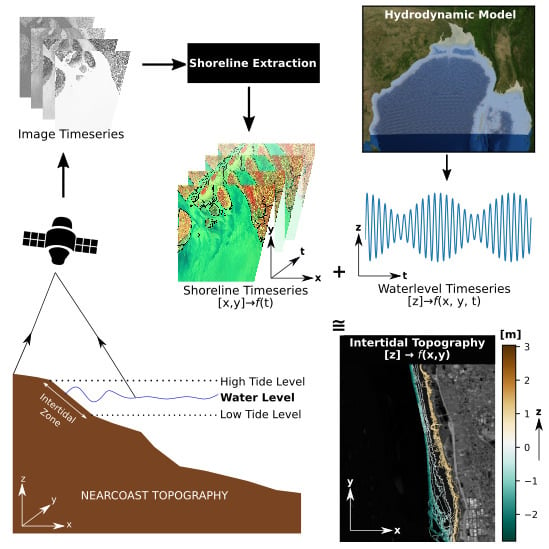
The present paper updates the method presented by Bergmann et al. [27], with several key advances. First, our method allows the use of high-resolution spaceborne imagery dataset. Here we demonstrate an application using Sentinel 2 imagery at 10 m resolution. This dataset is one order magnitude higher in resolution compared to 100 m in PROBA-V images. To the best of our knowledge, this freely available satellite dataset has never been used for deriving an intertidal DEM. Second, our method is fully automated and generic enough to be applicable to shorelines ranging from sandy to muddy, including the ability to resolve fine estuarine network and narrow creeks. Finally, our method combines the application of remote-sensing (used to infer the horizontal position of the waterlines at various phases of the tidal cycle) and high-resolution hydrodynamic modeling (used to vertically reference these waterlines) as suggested by [7]. Removing the requirement of any ancillary in situ data makes our method lightweight. As a test case, we present here an application of our method to infer a DEM of the near-shore intertidal zone over the whole Bengal delta.
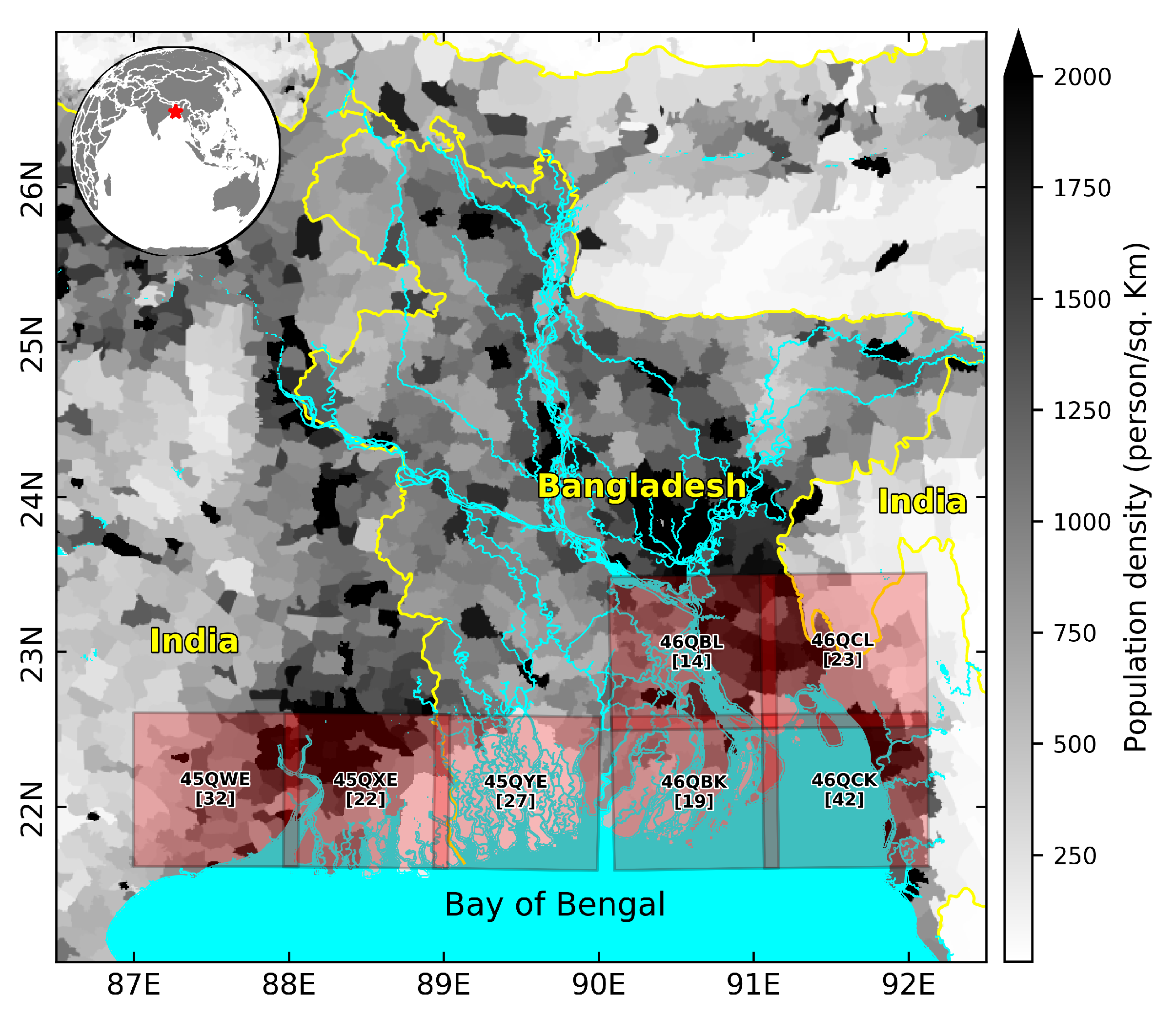
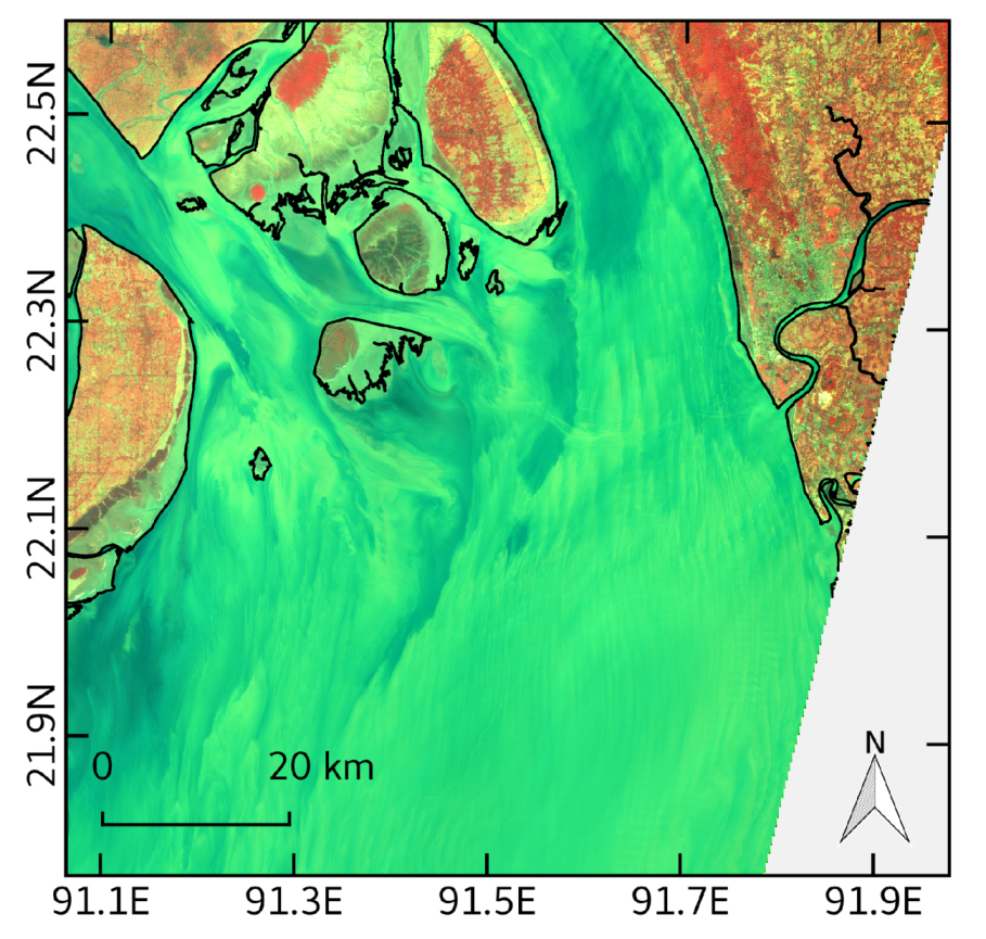
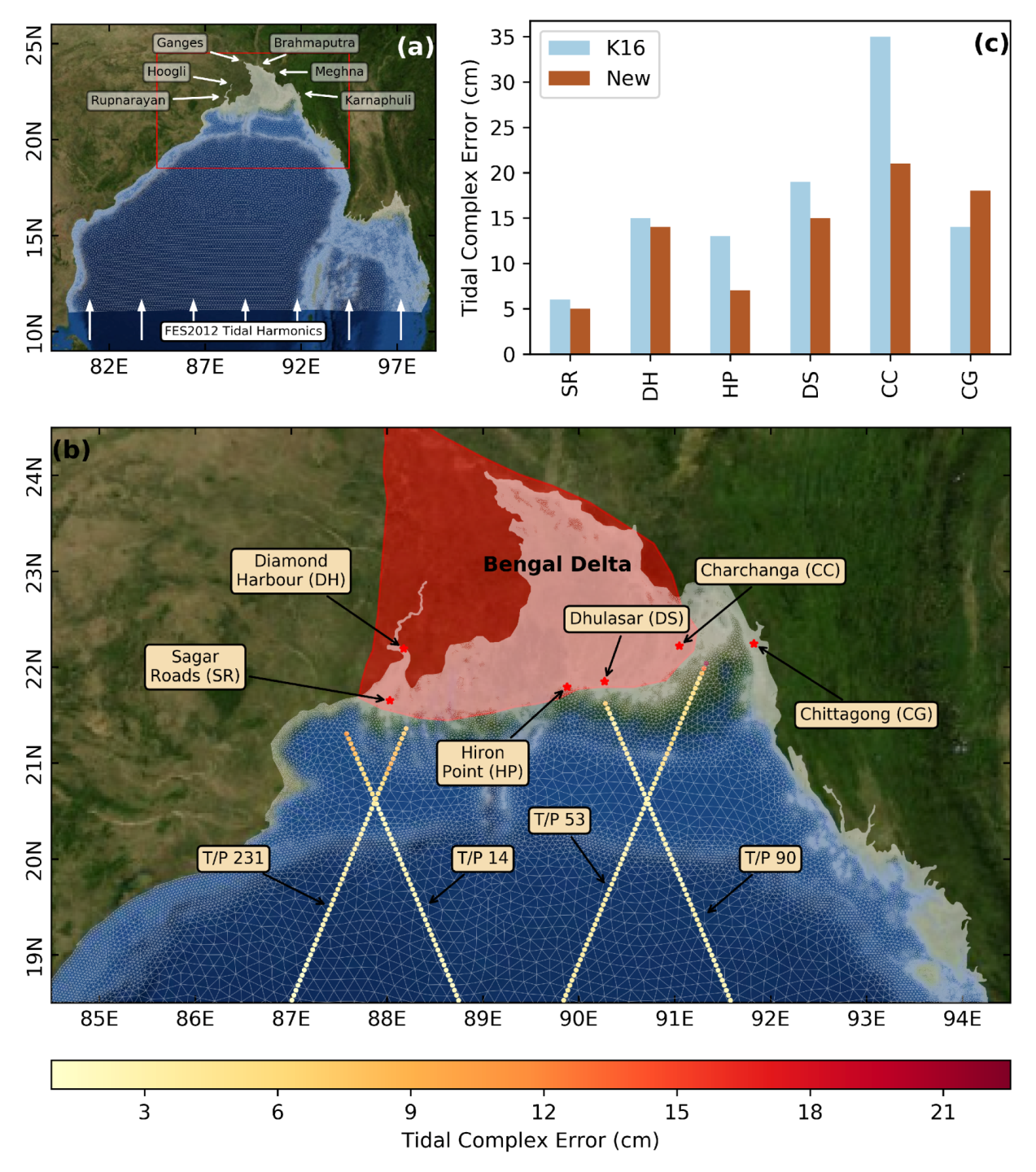
The coast of Bengal delta (Figure 1), across Bangladesh and India, is a well-known hotspot of coastal vulnerability. About 150 million people live in this region, characterized by a flat topography, with elevation typically inferior to 4 m above mean sea level (MSL) [29]. The near-shore ocean is characterized by a broad and shallow shelf with a mild slope in the order of 1/1000 to 1/5000, and a macro-tidal regime, with a tidal range in excess of 5 m in the North-Eastern part of the coast. The region is also prone to frequent tropical cyclones—on average, one major event in three years [30]. In the recent decades, three particularly devastating cyclones made landfall in this region, notably Gorky (1991), Sidr (2007), and Aila (2009) claiming about 140,000, 3400, and 190 lives, respectively. Due to the combination of low topography and high population, the coastal districts of Bengal delta are generally very prone to cyclone-induced flooding and associated loss of lives and assets [31].
The modeling of storm surge dynamics over this region is a challenging task for the scientific community. State-of-the-art numerical models can reproduce the estimated surge height, but they generally fail to reproduce the spatio-temporal evolution of the flooding [30]. Inaccurate and outdated representation of the near-shore bathymetry and land topography is identified as one of the most important factors that prevent from accurately reproducing the tidal dynamics, the cyclone surges characteristics as well as the coastal inundation patterns [30,33]. Using a bathymetry dataset derived from a large ensemble of digitized in situ hydrographic surveys, Krien et al. [29] significantly improved the representation of tidal hydrodynamics in the Bengal delta region. This dataset, however, essentially consists of point-wise soundings from shipborne surveys, which do not cover the very shallow-water zones (shallower than 2 m below MSL). This means that the whole intertidal area, which can be quite broad in this very flat region (up to several kilometers wide), are left void of up-to-date topographic data. However, it is well known that the knowledge of the intertidal topography is particularly important to realistically model the effect of wave set-up during storms and cyclones (e.g., [34]).
The Bengal coast is also characterized by erosion and accretion of the shoreline that manifests at various timescales ranging from days to decades [35]. These changes are particularly prominent in the mouth of Meghna estuary where the combined flow of Ganges, Brahmaputra, and Meghna is discharged. The large sediment discharge accompanies the runoff during the monsoon and then gets spread by far-reaching tidal currents as well as extreme events such as riverine floods and tropical cyclones [35,36]. Because of this dynamic nature, it is not feasible to perform repeated, extensive in situ hydrographic surveys over this extended deltaic region, thus making it a very interesting test case for applying our methodology.
The aim of this study is three-fold. First, we developed an automated procedure to extract waterlines from Sentinel 2 imagery. Second, we vertically referenced those shorelines using a hydrodynamic model of the area. This allows obtaining an intertidal topography. Third, we validated the resulting topography against in situ bathymetric observations harvested in a key-region of the Bay of Bengal. We present our algorithm to extract the shoreline in Section 2, which is followed by a description of our hydrodynamic modeling framework in Section 3. The resulting DEM over Bengal delta and its validation based on two independent in situ sounding dataset are presented in Section 4. Finally, we discuss our results and conclude our work in Section 5 and Section 6, respectively.

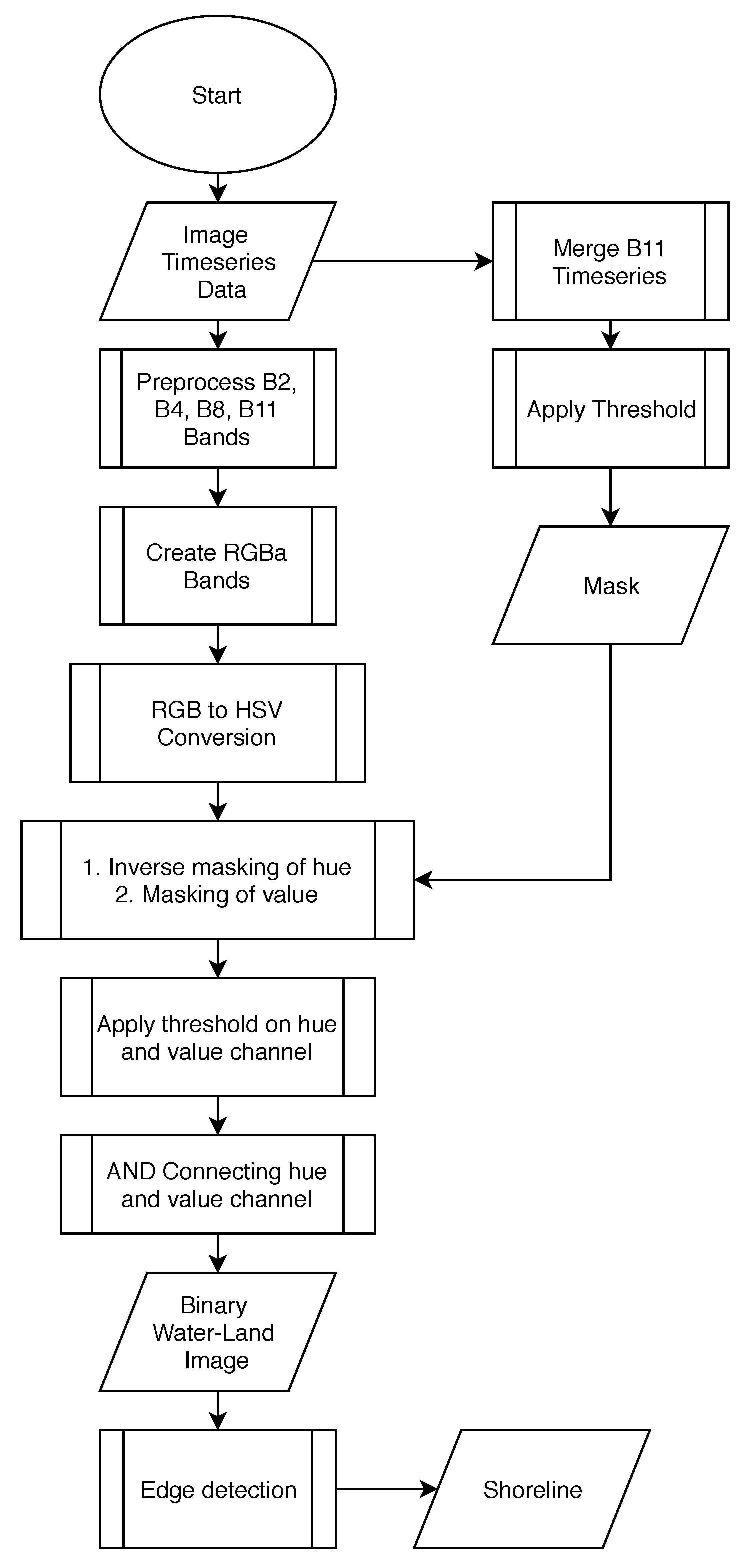
2. Shoreline Detection with Sentinel-2 Imagery

Sentinel-2 project was launched by European Space Agency to acquire high-resolution multi-spectral images with short revisit frequency. It comprises two satellites—Sentinel-2A and Sentinel-2B, successfully launched in 2015 and 2017. The objective of these missions is to provide long-term research-quality acquisition of land surface monitoring products. For the monitoring of water bodies, the use of Sentinel-2 is very appealing due to its open-access nature, high resolution (10 m), and short revisit period (about 10 days). Sentinel-2 satellites acquire data over 13 spectral bands—four bands (blue, green, red, near infra-red—NIR) at 10 m resolution and six other bands (including shortwave infra-red—SWIR) at 20 m resolution. Because of the large dataset size, Sentinel-2 products are distributed as tiles of 1 × 1 degree. We have used the Copernicus Sentinel-2 data processed at level 2A by CNES at Theia Land data center (https://theia.cnes.fr). The data is provided in separate GeoTIFF arrays for each of the spectral bands. All the individual tiles had been corrected from the atmospheric and adjacency effects, along with the detection of clouds and their shadows using MAJA processing chain [37].

2.1. Pre-Processing of the Dataset

For detection of shoreline, we have used the B2, B4, B8 and B11 bands, with the spectral properties provided in Table 1. We have selected images from the archive avoiding instances with prominent cloud cover (typically less than 10%). The images were already orthorectified and georeferenced. We have considered about three years of archive, from January 2016 to October 2018. This temporal selection encompasses on average 75 individual Sentinel-2 passes. Finally, we have considered seven tiles fully covering the coastal region of the Bengal delta. With 14 to 42 individual frames per tile, this selected dataset encompasses a large fraction of the observable tidal range. The coverage of the selected tiles, and the corresponding number of frames per tile are displayed in Figure 1. The corresponding satellite and timestamp information of the images are provided in Supplementary Tables S1–S7.
As mentioned in the previous section, our shoreline analysis approach is essentially an upgrade of the methodology presented in [27]. We updated their algorithm to make it compliant with the 10 m resolution of Sentinel-2 imagery, applicable to smaller tiles, and in a fully automated fashion. We consider the surface reflectance products identified by the prefix FRE (Flat Reflectance), corrected from both atmospheric and land slope effects.
Each band data file is coded as a 16-bit integer. The original reflectance value is found from dividing this integer dataset with 10,000. The pixels which were out of the field-of-view of the satellite pass are coded as - 10 , 000 . 
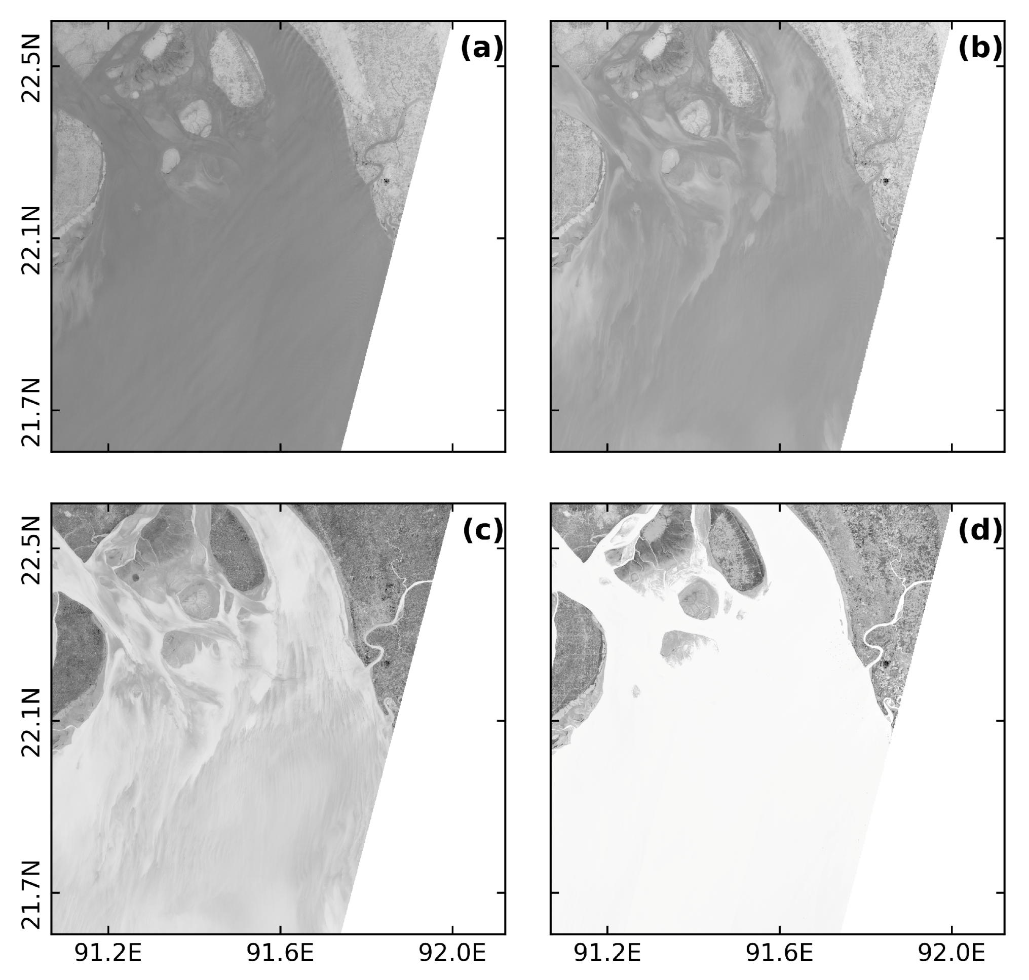
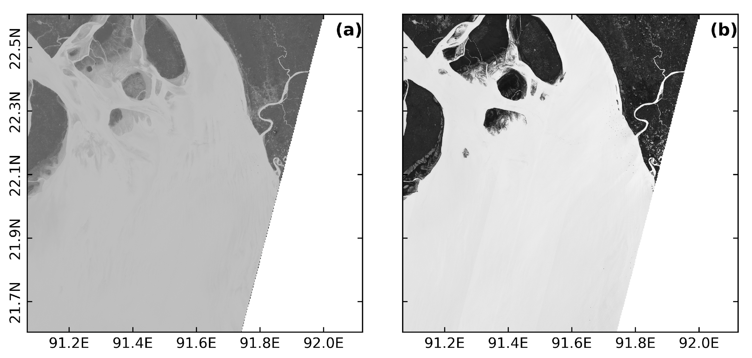
Figure 2 shows a sample of the Sentinel-2 bands used in this study.
Naturally, the illumination conditions vary from one scene to another for a given tile. On several scenes, we also noticed the presence of a few pixels with very high reflectance values. While we could not confirm the reason, at all instances these pixels correspond to some form of slanted roofs that might have induced powerful sun glint. To be consistent along the time series of the images, and to make our algorithm robust, we applied a pre-processing of the B11 band to remove these artificially bright pixels. We do so by capping the values at mean plus one standard deviation (std) on the upper side, i.e., restricting them within [0, mean+1*std]. Once the pre-processing of the B11 band is done, we apply a normalization of the dataset to [0, 1]. Finally, we use a nearest-neighbor approach to resample B11 band to 10 m from its original 20 m resolution. The B2, B4 and B8 bands are also normalized to [0, 1] for further processing.
In our approach, the B11 band serves as a transparency channel, the so-called alpha band. A synthetic red-green-blue-alpha space is constructed using B2, B4, B8 and B11 bands according to Equation (1).
r e d = ( 1 - B 11 n o r m ) + ( B 11 n o r m B 4 n o r m ) g r e e n = ( 1 - B 11 n o r m ) + ( B 11 n o r m B 8 n o r m ) b l u e = ( 1 - B 11 n o r m ) + ( B 11 n o r m B 2 n o r m )
The subscript n o r m refers to the pre-processed and normalized bands of the previous step. This allows taking the full advantage of land/water contrast captured in the B11 band while retaining the high-resolution information from the other three bands (Figure 3).
This synthetic RGBa (red-green-blue-alpha) bands in Figure 3 are converted to hue, saturation and value (HSV) color space following [28]. Among these three, we discard the saturation, which is essentially the intensity of the hue. This separation makes our algorithm indifferent to the various illumination conditions which are bound to happen for a multi-year archive. Only value and hue channels presented in Figure 4 are retained during the subsequent procedure.

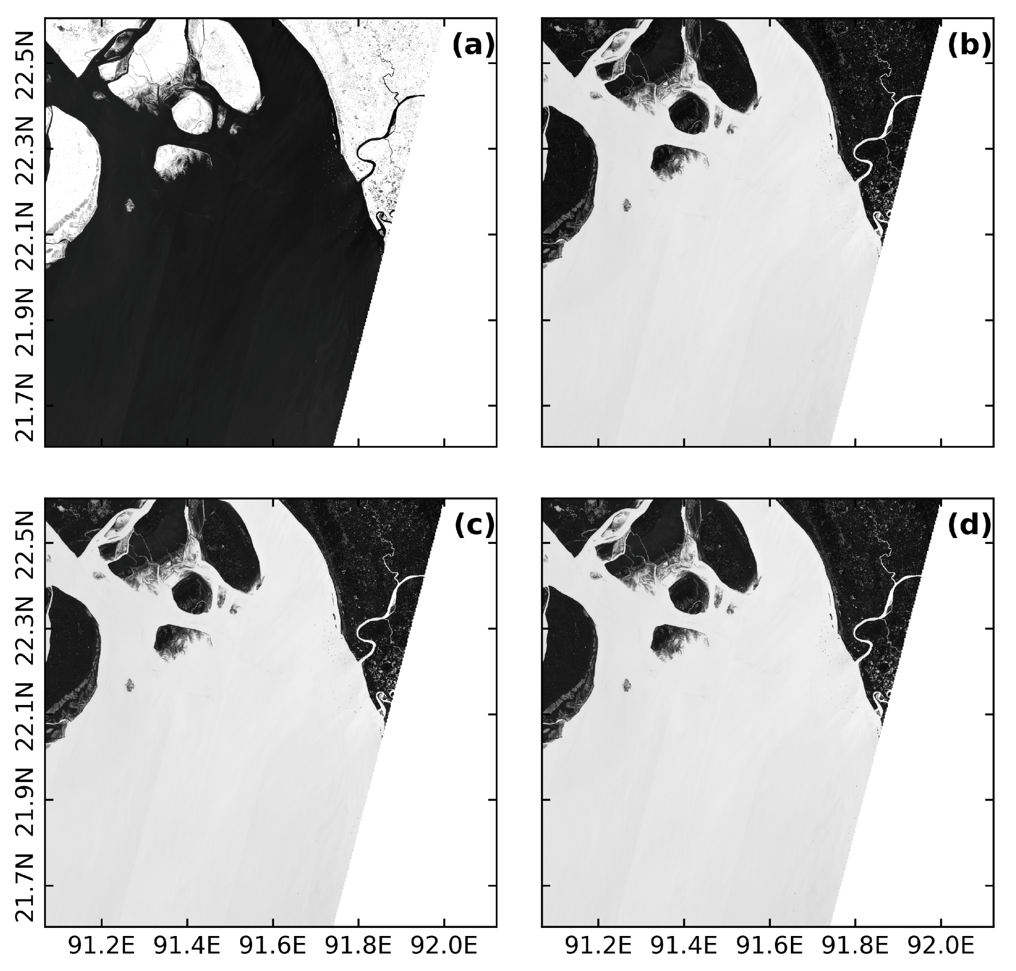
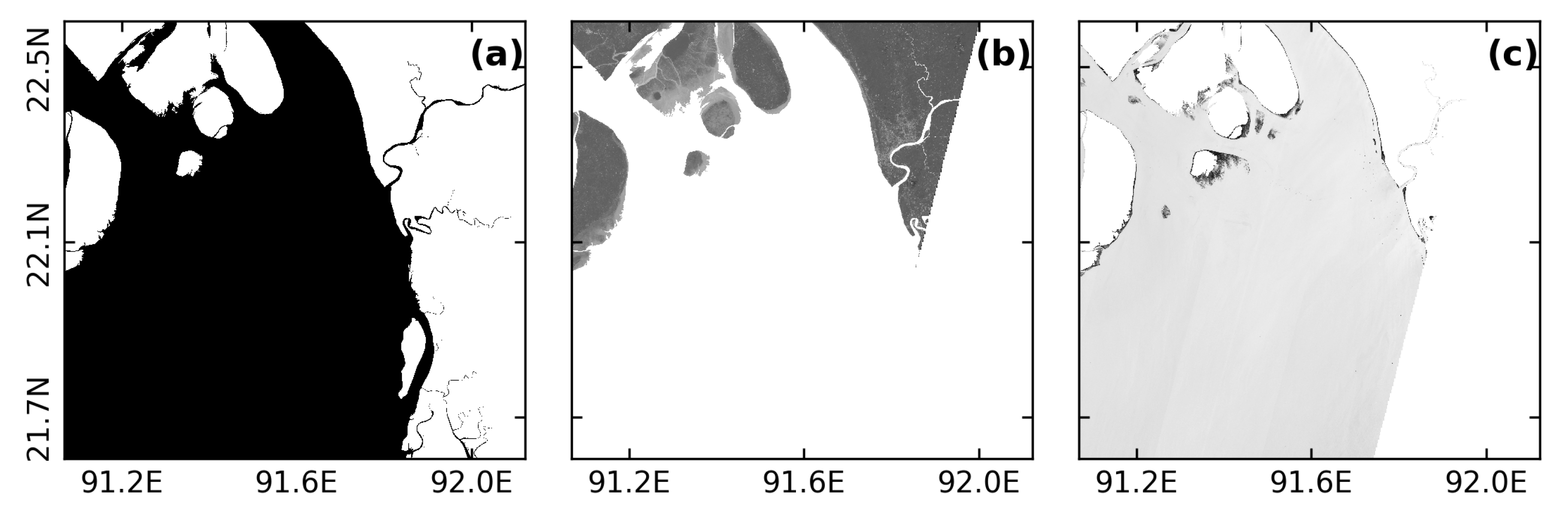
2.2. Coarse Water Mask

One of the essential steps in [27] is the preparation of a coarse water mask—only once for a given region—typically by hand, to roughly separate the water from land areas. This step allows guiding the subsequent accurate discrimination of water and land pixels along the land-water interface area. Preparing such a mask manually for a large area dataset such as our test case could be tedious. To automate the preparation of this mask we used the fact that B11 band consistently shows a very distinct contrast between land and water pixels. First we normalize the multiple acquisitions of B11 band, and merge all images by taking a pixel-by-pixel average. The first advantage of this merging is the filtering of any artefact that may be present in individual B11 band images (typically: localized stripes of under-illuminated pixels), thus retaining a clear separation between land and water with reduced noise. The second advantage is the full coverage of the tile by the accumulation of observed pixels. Each tile is essentially a clipped version of a continuous image along the swath of the satellite, thus yielding individual tiles which are not always fully covered during a pass (i.e., missing values). By combining all the available images, the presence of missing values is avoided.
To generate the water mask itself, we apply a threshold based on the standard deviation of the merged band, using Equation (2).
M a s k = 0 , where B 11 m e r g e d n m a s k std ( B 11 m e r g e d ) 1 , where B 11 m e r g e d < n m a s k std ( B 11 m e r g e d )
Here B 11 m e r g e d is the normalized and merged B11 band, std( B 11 m e r g e d ) is the standard deviation of the B 11 m e r g e d and n m a s k is a scalar factor. The output of this operation—mask—is a 2D array with water (1) and land (0) coarsely classified. For our application, we found that an n m a s k of 0.5 is suited for all the tiles. However, we recommend adjusting the value if needed, especially for tiles covering environments where the relative number of water pixels is very low (e.g., inland water body mapping).
The mask is further refined by application of a blob-removal procedure. For pixels identified as water (mask value of 1), any pixel blob with size smaller than 10,000 is replaced by land mask value (0). On the other hand, for the pixels identified as land (0), any blob with size smaller than 50,000 is replaced by water mask values (1). This process essentially removes the noise and results in a cleaner coarse segmentation of land and water. Once this final cleaning is done, we obtain the water mask. This process is done only once for a given set of images. One example of such mask for tile #46QCK is presented in Figure 5a.

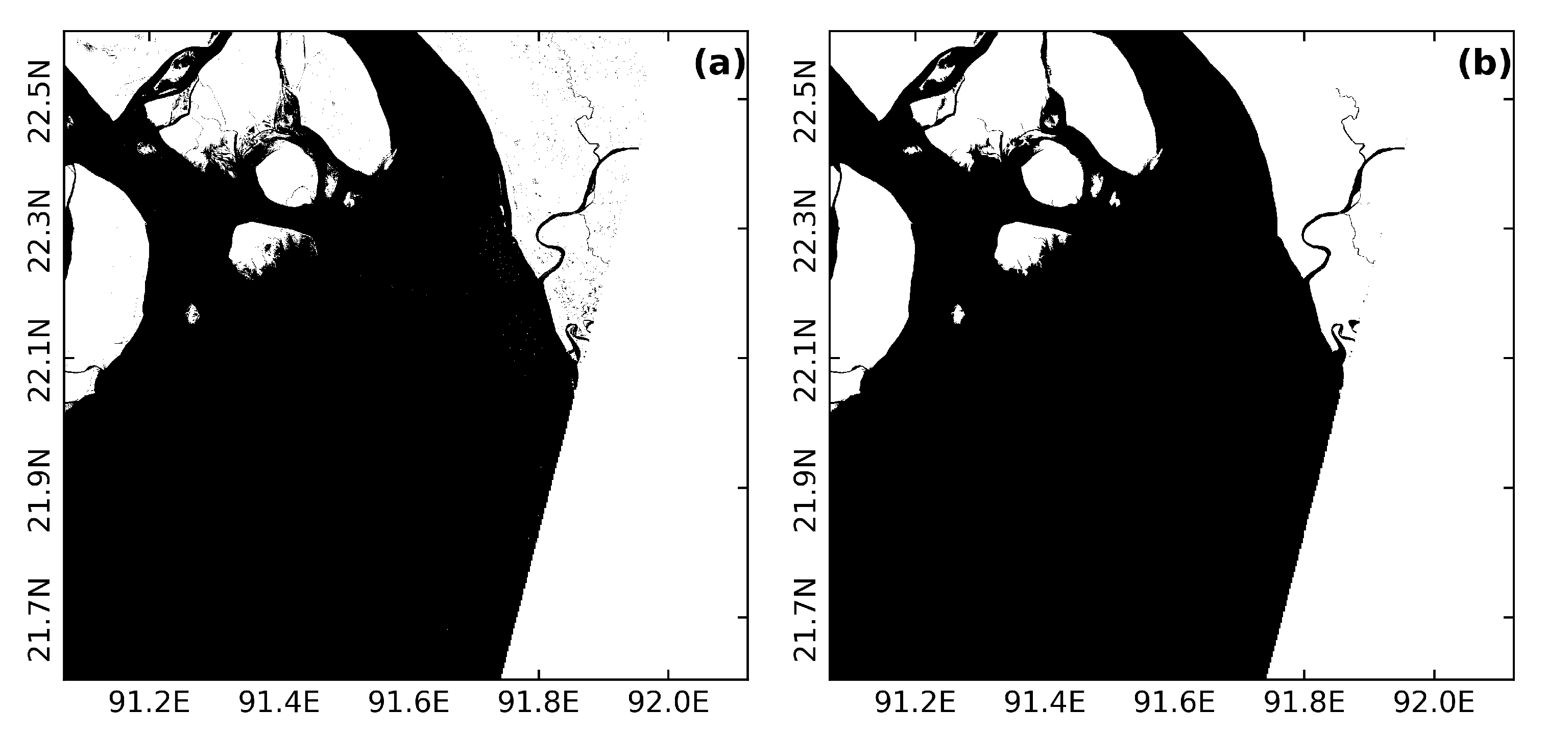
2.3. Shoreline Extraction

The basic principle of our shoreline extraction algorithm is to discriminate the pixels at the land-water interface guided by the pixel values of land and water zones coarsely separated by the above-defined coarse water mask. To identify the land-water interface, we first apply our water mask presented in Figure 5a to the hue and value channels. This mask is applied inversely on the hue channel (roughly retaining the land pixels, Figure 5b) and directly on the value channel (roughly retaining the water pixels, Figure 5c). Median and standard deviation are calculated for these masked channels, which are subsequently used to apply as a threshold on the images as defined by Equation (3).
BW h u e = ¬ ( I h u e < T h u e + n h u e σ h u e ) ( I h u e > T h u e - n h u e σ h u e ) BW v a l u e = ( I v a l u e < T v a l u e + n v a l u e σ v a l u e ) ( I v a l u e > T v a l u e - n v a l u e σ v a l u e )
Here the h u e and v a l u e subscript indicate the channel type, I is the original value of the channel before masking, BW (for Black–White) is the resulting binary channel. T and σ are the median and standard deviation, respectively. ¬ indicates the logical NOT operation.
Essentially Equation (3) separate land and water pixels at the interface by taking a window around the median of the inversely masked hue channel and of the masked value channel. The size of the window is controlled by n h u e and n v a l u e for hue channel and value channel, respectively. Lower scaling factor results in a stricter window of threshold, and vice versa. After several trials and visual inspection of the shorelines, we selected 0.5 and 3.0 for n h u e and n v a l u e respectively. These values are close to the values used by [27] for PROBA-V (0.4 and 5.0 for n h u e and n v a l u e respectively). The BW h u e and BW v a l u e channels are then AND-connected to obtain the final separation of land-water interface. The result of this operation is presented in Figure 6a.
At the final step, small-scale features are removed based on their size. We discard all water features smaller than 10,000 pixels in size inside land area; similarly, we remove all land features smaller than 10,000 pixels. These correspond to an area of 1 km 2 . This cleaning essentially removes all ships detected in the ocean as well as the smallest ponds detected inland. As a consequence of this cleaning, certain small-scale features such as coastal sandbars are also removed in our analysis, which are visible during low tide but submerged at high tide. The resulting image after our blob-removal procedure is presented in Figure 6b.
The final step of identifying the shoreline is applying an edge detector on the classified land-water binary image. To do this, the blob-removed binary water map obtained in the previous step is convoluted with a 3 × 3 Laplacian kernel following Equation (4).
S H ( i , j ) = p = 1 , 2 , 3 q = 1 , 2 , 3 K ( p , q ) B W c l e a n ( i - p + 1 , j - q + 1 )
Here, B W c l e a n is the clean binary water map, S H is the extracted shoreline map and K is the 2D kernel matrix defined as:
K = 0 - 1 0 - 1 4 - 1 0 - 1 0
The application of this edge detector in binary 2D space results in a raster image where only the pixels forming the water/land interface are left. The location of the shoreline is then defined at the center of these pixels and converted to longitude-latitude coordinates from the native UTM projection of the satellite images. An example of the resulting shoreline is shown in Figure 7.
This aforementioned procedure is summarized in the flowchart shown in 
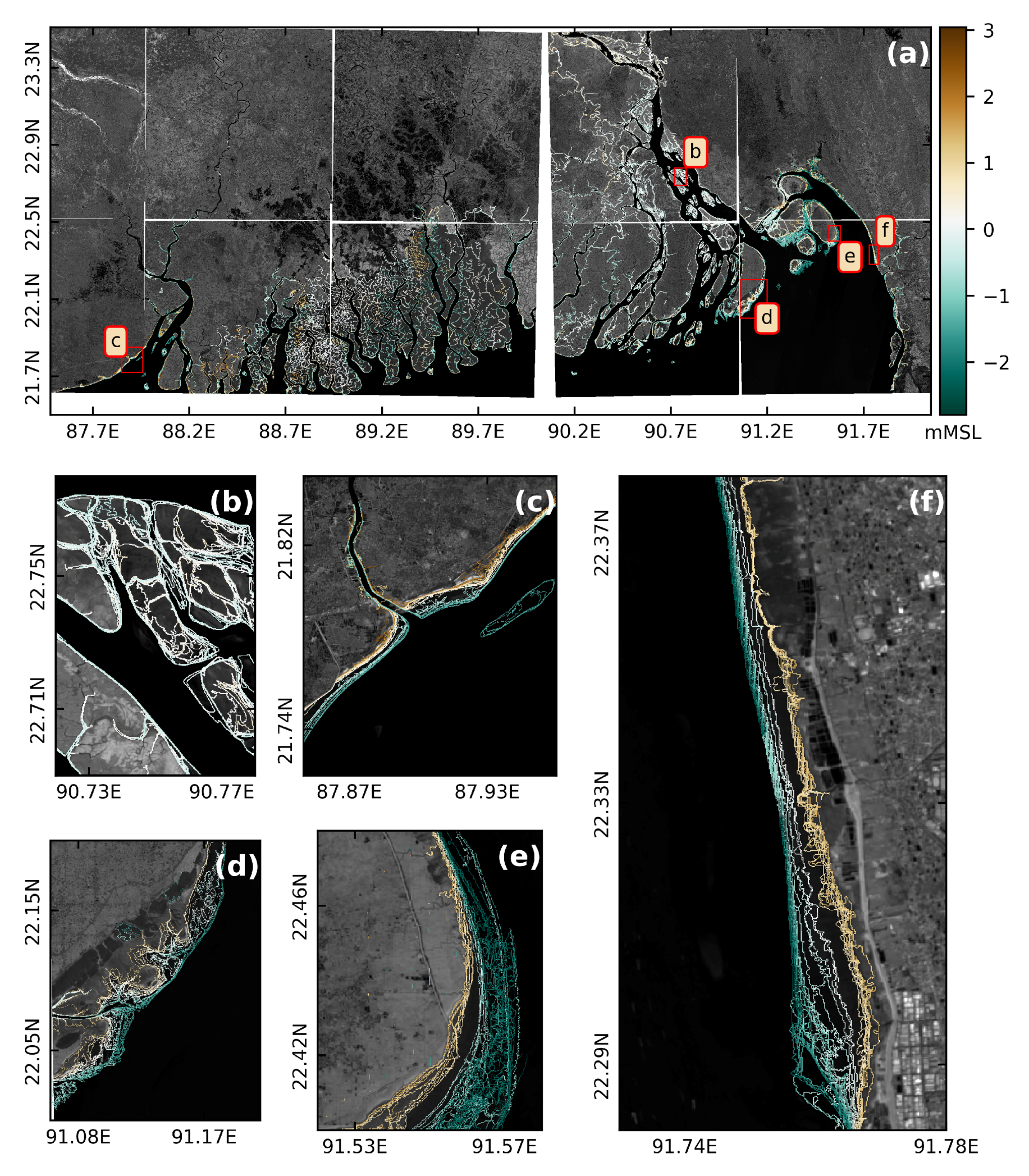
Figure 8. We apply this algorithm over the time series of selected Sentinel-2 images. Eventually a manual cleaning of the resulting water lines is performed to remove large, disconnected water bodies (particularly for tile #45QXE and tile #45QYE at their northern edge), which were too large to be removed using our blob-removal procedure. In most cases these disconnected water bodies are large shrimp farms. The vertical referencing of this timeseries of shorelines is described in the following section.
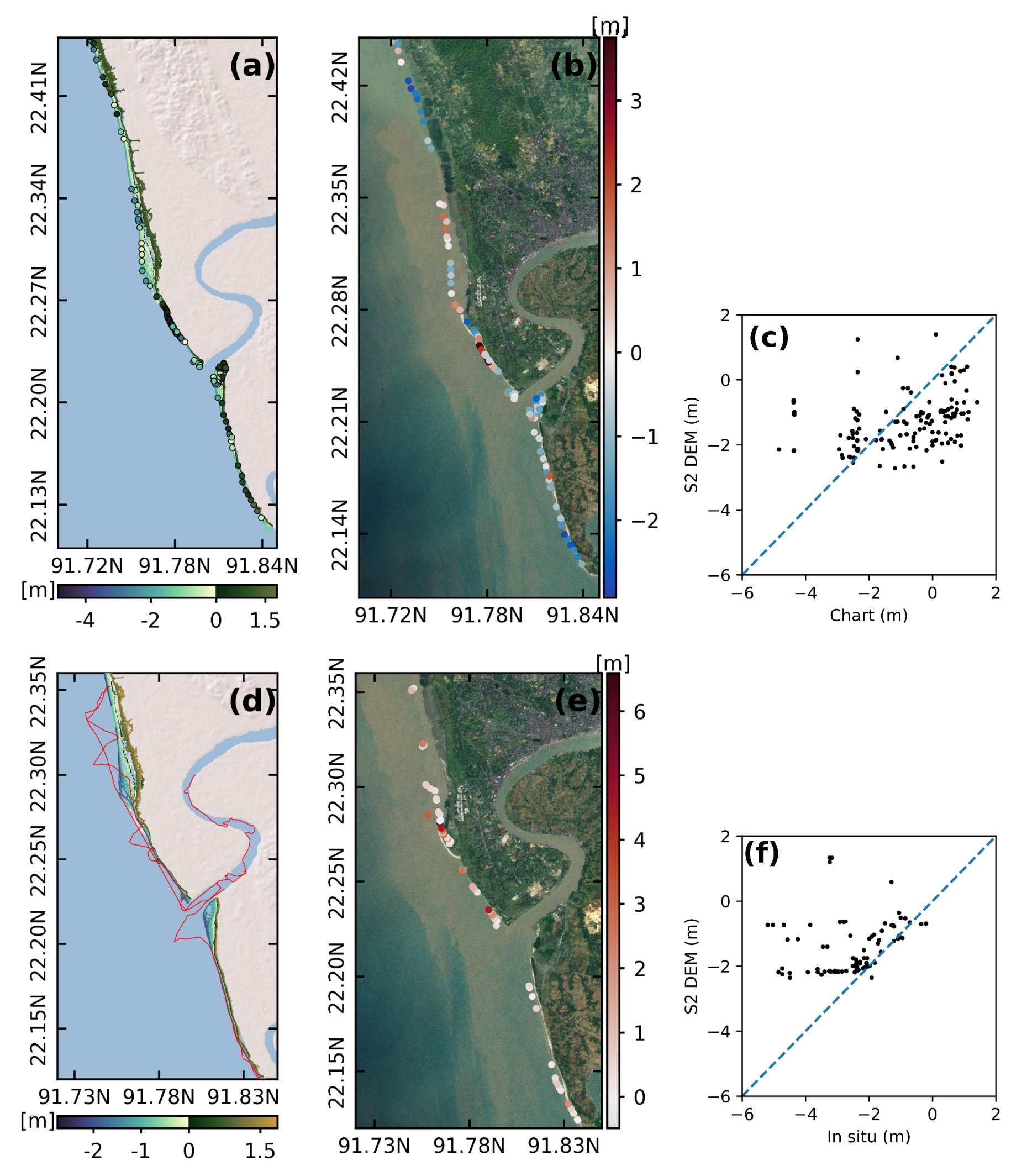
3. Vertical Referencing with Tidal Model

Applying the method described in the previous subsection over our time series of Sentinel-2 images results in a set of shorelines detected at various tidal phases (between low tide and high tide). Conceptually, assigning a vertical position to each of these shorelines would require the knowledge of the water level (as observed typically by a tide gauge) at each pixel along the shoreline, at the time of the acquisition of the corresponding image. Such estimates of the water level can be achieved by various means—including using a local tide gauge to estimate the evolution of water level in the time and space, using a publicly available tidal atlas to predict the tidal water evolution, or using a full-fledged hydrodynamic model running over the time span of the acquired image set. For example, Bergmann et al. [27] used several local tide gauges to estimate the evolution of water level in time and space by spatio-temporal extrapolation. One could also rely on any good-quality tidal atlas available over the area to predict the tidal water evolution at the location and time of observation of the retrieved shorelines. We hereafter follow this latter option, based on a hydrodynamic tidal modeling framework we purposely developed for accurate tidal water-level prediction over the Bengal delta.

3.1. Hydrodynamic Tidal Modeling Framework

We have used SCHISM (Semi-implicit Cross-scale Hydroscience Integrated System Model) [38], a derivative code of SELFE (Semi-Implicit Eulerian-Lagrangian Finite Element) model, originally developed by Zhang and Baptista [26]. This modeling framework solves the 3D shallow-water equations for ocean flow and sea level, using finite-element and finite-volume schemes. It has been designed and used for many geographical areas including our region of interest, covering a broad range of spatial scales ranging from ocean basins (e.g., [29,38]) to very shallow lagoons and estuaries (e.g., [39,40]) as well as from short temporal scales (e.g., tsunamis [41]) to seasonal and inter-annual scales (e.g., [42]).
The tidal model presented in this study is a major update to the one presented in [29]. Considering the importance of the near-shore bathymetry in the realism of the simulated water-level variability, and the successful use of navigational charts in the bathymetric dataset used by [29] to define the model geometry, we updated the bathymetry described in [29] with 34 new navigational charts over the northern Bay of Bengal. This process resulted in 77,000 manually digitized sounding points. This bathymetry dataset is then used to develop the model mesh showed in Figure 9.
The model mesh is triangular, unstructured (viz. with varying spatial resolution) discretized based on the wave propagation criterion and bathymetric gradient [30]. The unstructured grid allows refining considerably the horizontal resolution in the shallow coastal ocean that forms the focus of the present study (Figure 9). The model mesh extends from 11 ° N to 24 ° N, and comprises about 600,000 grid points. The resolution of the element ranges from 250 m in the intertidal area at the lower part of the delta (above 20 ° N) to 15 km in the deep offshore ocean. Along the shorelines of India and Myanmar (south-western and south-eastern edges of the model domain), the near-shore resolution ranges from 1.7 km to 3.5 km. The model resolution is found to be sufficient to capture the geometry of the polders and dikes that are ubiquitous in the southern part of the delta. For the temporal integration of the model, a 300 s time step was chosen after a few sensitivity tests, although in our modeling framework a time step ranging from 200 to 400 s was found to be equally performing, thanks to robust numerics of the model formulation.
The model is forced with three different forcings—tidal potential for whole domain, tidal elevation at the southern open boundary and river freshwater fluxes at the upstream riverine open boundaries. Figure 9a shows the locations of these open boundaries. The choice of tidal constituents for tidal potential and tidal elevation at the southern boundary is kept essentially the same as in the configuration of [29] with some addition. The amplitude and phase of the tidal constituents prescribed at the southern boundary are extracted from FES2012 atlas [43]. To reproduce the seasonal changes in water level observed in the northern Bay of Bengal, we have also imposed an annual cycle of 35 cm amplitude along the southern open boundary in the same manner as Tazkia et al. [42]. The river freshwater fluxes—one of the ingredients of coastal water-level variability [44]—are prescribed in the inland open boundaries. We have prescribed rated daily discharges at the upstream boundaries of Ganges and Brahmaputra rivers with observed data provided by Bangladesh Water Development Board (BWDB) for 2014. We have also imposed a monthly climatology of discharge of Hooghly river based on the discharge observed at Farakka [45], and a monthly climatology of discharge of Karnaphuli river based on the discharge observed at the Kaptai hydro-electric power plant [46]. We have applied Flather boundary condition [47] at Meghna and Rupnarayan River allowing the tide to propagate freely outside the computational domain. At the remaining coastal boundaries, no normal flow is assumed for the velocity boundary condition. The bottom friction, which is represented through a Manning coefficient n in our modeling framework, is applied in a similar fashion to [29] based on the bathymetric depth in the ocean (n = 0.013 for regions shallower than 20 m and n = 0.02 otherwise). A value of n = 0.01 is imposed for all the rivers.

3.2. Tidal Water-Level Estimation for Vertical Referencing

The tidal analysis on the unstructured grid is performed using COMODO tools developed at LEGOS [48] on simulated hourly water level from December 2013 to January 2015 (14 months). In total, 33 constituents (M2, S2, O1, K1, K2, L2, J1, E2, 2N2, La2, M3, M4, M6, M8, Mf, MKS2, Mm, MN4, MS4, MSf, Mtm, Mu2, N2, N4, Nu2, P1, Q1, R2, S1, S2, S4, T2, Sa, Ssa), as well as the long-term mean (Z0) is extracted. This essentially amounts to a new tidal atlas for the northern Bay of Bengal. The quality of the tide is assessed using complex error calculated from four dominant tidal constituents—M2, S2, O1, and K1. The assessment is carried out based on two independent datasets: tidal constants obtained from in situ tide gauges, and from spaceborne altimetry. The latter dataset is the CTOH product, available on http://ctoh.legos.obs-mip.fr/data/coastal-products/coastal-products-1/tidal-constants (see this website for further details on the altimetric processing). Our tidal atlas appears globally consistent with the spaceborne product, with errors in the offshore domain of order 3 cm, increasing shoreward along all altimetric tracks, but nowhere exceeding 23 cm. Figure 9c shows the complex error estimation for the tide gauges shown in Figure 9b and its comparison with the results in [29]. At the gauge stations we have found a substantially reduced error estimate, particularly at the central region stations of Charchanga (CC) and Hiron Point (HP). The overall accuracy of our tidal atlas is of order 5 cm to 20 cm, which is unprecedented over our region, and in line with the performance of state-of-the-art tidal atlases along the best-documented shorelines [49].
For vertical referencing of the shorelines extracted in Section 2, we used the full set of 33 constituents from our atlas to generate the water level at the timestamps of the image acquisition by Sentinel-2 using COMODO tools. For each inferred shoreline from the imagery, the water level corresponding to each shoreline pixel is found in the model tidal prediction through a nearest-neighbor interpolation technique. Although most of the shoreline pixels are relatively close to water pixels, there are some instances where the tidal model does not cover the full extent of the tile (particularly the inland rivers in #45QWE). To be consistent, the detected shoreline pixels where the nearest neighbor is more than 6 km were discarded during the referencing process. This distance threshold is selected based on the assumption of relatively low water-level gradient and typical cross-river distance. At the shorelines with high bathymetric gradient, such as cliff shores, where the shoreline change between low tide and high tide is sub-pixel scale (<10 m), the lowest elevation value is registered for the various tidal stages.

4. Results

4.1. Intertidal DEM

Figure 10a presents our DEM over the whole domain overlaid on merged B11 band used in this study. Our DEM maps 1134 km 2 intertidal area along the coast of Bengal delta at 10 m resolution. The horizontal extent of our DEM is in order of 600,000 km 2 . The mapped intertidal topography ranges from - 3 m to 3 m with respect to MSL. To the best of our knowledge, the geographical coverage of our product, along with the level of details visible at fine scale throughout the deltaic river network, is unprecedented over our area. Figure 10b–f provides close-up views of several key-locations of the delta, contrasting the eastern active side of the delta (Meghna estuary, Figure 10b), the western dead side of the delta (Hooghly estuary, Figure 10c), the muddy islands located in the immediate vicinity of the mouth of Meghna (Hatiya Island, Figure 10d and Sandwip Island, Figure 10e), and the sandy beach region of Chittagong analyzed by [27] (Figure 10f).
Compared to the Hooghly estuary, Meghna estuary shows a much richer population of islands. The topographic slopes revealed by our dataset along the periphery of the south-eastern muddy islands (Hatiya and Sandwip, Figure 10d,e) are typically much milder than those of the islands located in the Hooghly estuary (Figure 10c). The Chittagong close-up in Figure 10f can be directly compared with the corresponding map in Figure 13 of [27]. It is seen that our waterlines are much smoother compared to [27], despite the ten-fold increased resolution of our dataset. This indicates that our approach has injected an appreciable amount of information, even at decameter scales, taking over the small-scale noise and artefacts of our detection procedure to be expected from the higher resolution images. Also, the numerous instances of overlapping and intersecting isolines seen in [27] DEM are mostly unseen in the new DEM, which suggests that our updated procedure and high-resolution dataset altogether yield a physically more consistent retrieval. Given the pivotal role of decametric-scale near-shore bottom slope in the coastal ocean hydrodynamics (e.g., [34]), our product thus offers promising perspectives to coastal ocean modelers.

4.2. Validation of Our DEM

Beyond the qualitative—though reassuring—features discussed above, it is timely to carry out a quantitative assessment of our DEM against independent in situ observations. We did so by relying on the three nautical charts from Bangladesh Navy Hydrographic and Oceanographic Centre (chart #1251, #3001, and #3509, based on surveys conducted in 2012–2015). We considered all charts point-wise soundings falling in the intertidal area, and co-located them with our own DEM. This resulted in 145 comparison points, displayed in Figure 11a. Figure 11b shows the error at individual points. For further visual comparison, a scatter plot between our DEM vs the in situ chart observations are shown in Figure 11c. The root-mean square difference between our DEM and the in situ soundings is close to 1.5 m, which is similar to [27]. However, our DEM presents a deep bias with the in situ soundings of 0.36 m. This value has the same sign, but is much smaller than the 1.2 m bias observed by [27]. This value is also in line with the typical bias of similar approaches in other regions [5].
The aforementioned chart soundings dataset was produced from oceanographic vessels, which essentially leave the shallowest parts of the intertidal region void of observations. Hence we decided to collect a set of primary observations in this near-shore part of the intertidal area. This was done through a shipborne hydrographic survey conducted on 11–13 February 2018 along the track displayed in Figure 11d. The measurements were operated through an acoustic echo-sounder, vertically referenced by an on-board GNSS using precise-point-positioning (PPP) processing. The trajectory usefully complements the spatial coverage of the previous dataset. Indeed, thanks to the small draught of the ship we used, and the high tide conditions during parts of the survey, it was possible to sail shoreward of the 0 m isobath in several occasions. The typical horizontal resolution of the in situ dataset is 50 m, which is close to the resolution of our spaceborne DEM. We collocated this dataset with our spaceborne DEM and could find 82 comparison points. It was found that our DEM presents a shallow bias of 1.19 m, and a root-mean square difference of 1.39 m, similar to the value found when considering the navy soundings. All these values of bias and standard error lie within the commonly accepted accuracy of in situ soundings (estimated to 1–2 m) [50]. These error estimates and the visibly consistent features mentioned in the previous paragraph (viz. absence of isobaths intersections) give confidence in the overall validity of our new DEM.

5. Discussion

Our algorithm essentially builds on a well-known and tested methodology [6,27]. However, our method uses a new generation of satellites and is computationally lighter and automated. We also demonstrated the utility of a good hydrodynamic modeling framework, instead of depending on ancillary in situ data. The application of our algorithm to the imagery archive of Sentinel-2 over the Bengal delta resulted in a large-scale high-resolution intertidal DEM, encompassing the whole delta. The large area of the region we considered, of order 600,000 km 2 , did not induce any computational issue thanks to the lightness of the proposed procedure. Typically, it takes 6–7 h on a laptop computer to process the Sentinel-2 archive and generate the DEM covering such an extended region. Based on both navy soundings and dedicated primary observations, we could conclude that our DEM has an accuracy order of 1 m, which is in line with the state-of-the-art estimates produced in this region or in similar environments [14,27].
There are some assumptions in this approach which should be kept in mind. We assume that the water-level changes are driven by oceanic tide only. To validate our assumption, we replaced our tidal atlas by an ocean model hindcast, accounting for the atmospheric forcing (wind speed and air pressure) in addition to the tidal forcing. This did not appreciably change our resulting DEM, thus not shown here. The reason behind this is that the selection of cloud-free images typically dictates fair weather conditions associated with minor non-tidal sea level variability. However, in other coastal regions of the world ocean, where the tidal range is weaker than in ours and/or where the effects of atmospheric variability on sea level become prominent, it may be required to adopt this kind of more sophisticated approach to make the most of Sentinel-2 and similar imagery products.
For vertical referencing using the model derived tidal water level, we co-located each shoreline pixel to nearest always-wet hydrodynamic model node. This assumes that the water-level gradient is negligible in the scale of our hydrodynamic model (typically 300 m).
Additionally, our approach essentially assumes that the bathymetry of the intertidal zone is stationary over the duration of the imagery archive, which is rather small (about 3 years) in our case. However, in the case of coastal zones with prominent erosion/accretion, the long-term morphological changes might significantly distort the resulting DEM, which would result in waterlines artificially stretched, clubbed, and/or intersecting one another. In such circumstances a methodology more refined than ours may be required. Typically, a workaround approach could be to segregate the imagery archive in consecutive epochs over which the morphological changes can be neglected, then analyzing each of these periods individually following our methodology. This would allow identifying, beyond the intertidal DEM, the regions of marked erosion or accretion.
During the final step of our image processing, we have filtered the images to discard land and water features smaller than a certain size. In our case-study of Bengal delta, we have chosen 10,000 pixels (1 km 2 ) to filter ships and small inland ponds and retaining the ocean-land shorelines. This value is essentially subjective and depends on the objective of the analysis. For example, if the objective of the image processing is to map the inland water bodies, one may choose to remove this filtering altogether.
Based on the analysis over a broad region and multiple image tiles, we conclude that the n h u e and n v a l u e parameters used in our study are robust and well suited irrespective of the study area. For any user willing to apply our algorithm on Sentinel-2 imagery, these values should remain as reported in this paper. Our ambition for this algorithm is also to be used for another dataset than Sentinel-2. Thus, we keep open the possibility to tune these parameters for sensors with radiometric characteristics different from Sentinel-2 mission.

6. Conclusions

In this work, we present a method to infer an intertidal DEM from Sentinel-2 multi-spectral imagery and hydrodynamic modeling. Our approach, being easy to implement and automate, was designed to be readily usable in any region worldwide.
The near-shore hydrodynamics, particularly during cyclones and storm surges, is an active field of investigation [30,33]. While waves play an important role in the flooding, the available topographic information over Bengal delta are generally of inadequate resolution to study the small-scale processes. In future studies, our new DEM could be useful for high-resolution near-shore wave modeling over the Bengal delta. The tools and methodology presented here can be extended to study the morphodynamics of coastal regions, over broad geographical extent such as the large deltas.
Being computationally light, it paves the way towards the new generation of high-resolution spaceborne imagery. Our methodology is expected to be directly applicable to the meter-scale products already available from SPOT or PLEIADES missions, or to the future CO3D constellation expected in 2022. It also allows reanalysis of past missions in the same automated fashion presented here.
Our approach yields a DEM that can also be used to cross-evaluate other near-shore topography datasets, such as the global digital surface model ALOS World 3D (AW3D30, 30 m of resolution, [51]) or newly available topography datasets provided by ICESat-2 (Ice, Cloud, and Land Elevation Satellite-2) altimetry mission carrying the advanced topographic laser altimeter system (ATLAS) instrument, which is very promising for estimating the elevation of coastal and intertidal areas at low tide [5].

Supplementary Materials

The following are available online at https://www.mdpi.com/2072-4292/11/24/2888/s1. The list of Sentinel 2 images are provided as supplementary materials. The source code of the python toolbox used for analysis is available at https://github.com/jamal919/pyIntertidalDEM.

Author Contributions

Conceptualization, L.T. and F.D.; methodology, F.D. and M.J.U.K.; software, M.N.A. and M.J.U.K.; validation, M.J.U.K., M.I. and S.C.; writing—original draft preparation, F.D. and M.J.U.K.; writing—review and editing, F.D., L.T., Y.K., A.S.I., F.P.; visualisations, M.J.U.K.

Funding

This research was funded by CNES through the “BANDINO” TOSCA grant.

Conflicts of Interest

The authors declare no conflict of interest.

References

  1. Hallegatte, S.; Green, C.; Nicholls, R.J.; Corfee-Morlot, J. Future flood losses in major coastal cities. Nat. Clim. Chang. 2013, 3, 802–806. [Google Scholar] [CrossRef]
  2. Murray, N.J.; Phinn, S.R.; DeWitt, M.; Ferrari, R.; Johnston, R.; Lyons, M.B.; Clinton, N.; Thau, D.; Fuller, R.A. The global distribution and trajectory of tidal flats. Nature 2018, 565, 222–225. [Google Scholar] [CrossRef] [PubMed]
  3. Eakins, B.W.; Grothe, P.R. Challenges in Building Coastal Digital Elevation Models. J. Coast. Res. 2014, 297, 942–953. [Google Scholar] [CrossRef] [Green Version]
  4. Mason, D.C.; Gurney, C.; Kennett, M. Beach topography mapping—A comparsion of techniques. J. Coast. Conserv. 2000, 6, 113–124. [Google Scholar] [CrossRef]
  5. Salameh, E.; Frappart, F.; Almar, R.; Baptista, P.; Heygster, G.; Lubac, B.; Raucoules, D.; Almeida, L.P.; Bergsma, E.W.J.; Capo, S.; et al. Monitoring Beach Topography and Nearshore Bathymetry Using Spaceborne Remote Sensing: A Review. Remote Sens. 2019, 11, 2212. [Google Scholar] [CrossRef] [Green Version]
  6. Mason, D.C.; Davenport, I.J.; Robinson, G.J.; Flather, R.A.; McCartney, B.S. Construction of an inter-tidal digital elevation model by the ‘Water-Line’ Method. Geophys. Res. Lett. 1995, 22, 3187–3190. [Google Scholar] [CrossRef]
  7. Mason, D.; Hill, D.; Davenport, I.; Flather, R.; Robinson, G. Improving inter-tidal digital elevation models constructed by the waterline technique. Eur. Space Agency Publ. 1997, 414, 1079–1082. [Google Scholar]
  8. Zhao, B.; Guo, H.; Yan, Y.; Wang, Q.; Li, B. A simple waterline approach for tidelands using multi-temporal satellite images: A case study in the Yangtze Delta. Estuar. Coast. Shelf Sci. 2008, 77, 134–142. [Google Scholar] [CrossRef]
  9. Tseng, K.H.; Kuo, C.Y.; Lin, T.H.; Huang, Z.C.; Lin, Y.C.; Liao, W.H.; Chen, C.F. Reconstruction of time-varying tidal flat topography using optical remote sensing imageries. J. Photogramm. Remote Sens. 2017, 131, 92–103. [Google Scholar] [CrossRef]
  10. Liu, Y.; Huang, H.; Qiu, Z.; Fan, J. Detecting coastline change from satellite images based on beach slope estimation in a tidal flat. Int. J. Appl. Earth Obs. Geoinf. 2013, 23, 165–176. [Google Scholar] [CrossRef]
  11. Mason, D.; Garg, P. Morphodynamic Modelling of Intertidal Sediment Transport in Morecambe Bay. Estuar. Coast. Shelf Sci. 2001, 53, 79–92. [Google Scholar] [CrossRef]
  12. Scott, T.; Mason, D. Data assimilation for a coastal area morphodynamic model: Morecambe Bay. Coast. Eng. 2007, 54, 91–109. [Google Scholar] [CrossRef]
  13. Sagar, S.; Roberts, D.; Bala, B.; Lymburner, L. Extracting the intertidal extent and topography of the Australian coastline from a 28 year time series of Landsat observations. Remote Sens. Environ. 2017, 195, 153–169. [Google Scholar] [CrossRef]
  14. Bishop-Taylor, R.; Sagar, S.; Lymburner, L.; Beaman, R.J. Between the tides: Modelling the elevation of Australia’s exposed intertidal zone at continental scale. Estuar. Coast. Shelf Sci. 2019, 223, 115–128. [Google Scholar] [CrossRef]
  15. Niedermeier, A.; Romaneessen, E.; Lehner, S. Detection of coastlines in SAR images using wavelet methods. IEEE Trans. Geosci. Remote Sens. 2000, 38, 2270–2281. [Google Scholar] [CrossRef]
  16. Heygster, G.; Dannenberg, J.; Notholt, J. Topographic Mapping of the German Tidal Flats Analyzing SAR Images With the Waterline Method. IEEE Trans. Geosci. Remote Sens. 2010, 48, 1019–1030. [Google Scholar] [CrossRef]
  17. Li, Z.; Heygster, G.; Notholt, J. Intertidal Topographic Maps and Morphological Changes in the German Wadden Sea between 1996–1999 and 2006–2009 from the Waterline Method and SAR Images. IEEE J. Sel. Top. Appl. Earth Obs. Remote Sens. 2014, 7, 3210–3224. [Google Scholar] [CrossRef]
  18. Work, E.; Gilmer, D.S. Utilization of satellite data for inventorying prairie ponds and lakes. Photogramm. Eng. Remote Sens. 1976, 42, 685–694. [Google Scholar]
  19. Rundquist, D.C.; Lawson, M.P.; Queen, L.P.; Cerveny, R.S. THE relationship between summer-season rainfall events and lake-surface area. J. Am. Water Resour. Assoc. 1987, 23, 493–508. [Google Scholar] [CrossRef]
  20. Tucker, C.J.; Sellers, P.J. Satellite remote sensing of primary production. Int. J. Remote Sens. 1986, 7, 1395–1416. [Google Scholar] [CrossRef]
  21. McFeeters, S.K. The use of the Normalized Difference Water Index (NDWI) in the delineation of open water features. Int. J. Remote Sens. 1996, 17, 1425–1432. [Google Scholar] [CrossRef]
  22. Xu, H. Modification of normalised difference water index (NDWI) to enhance open water features in remotely sensed imagery. Int. J. Remote Sens. 2006, 27, 3025–3033. [Google Scholar] [CrossRef]
  23. Xu, Z.; Jin Kim, D.; Kim, S.H.; Cho, Y.K.; Lee, S.G. Estimation of seasonal topographic variation in tidal flats using waterline method: A case study in Gomso and Hampyeong Bay, South Korea. Estuar. Coast. Shelf Sci. 2016, 183, 213–220. [Google Scholar] [CrossRef] [Green Version]
  24. Jain, S.K.; Singh, R.D.; Jain, M.K.; Lohani, A.K. Delineation of Flood-Prone Areas Using Remote Sensing Techniques. Water Resour. Manag. 2005, 19, 333–347. [Google Scholar] [CrossRef]
  25. Frazier, P.S.; Page, K.J. Water body detection and delineation with Landsat TM data. Photogramm. Eng. Remote Sens. 2000, 66, 1461–1468. [Google Scholar]
  26. Zhang, Y.; Baptista, A.M. SELFE: A semi-implicit Eulerian–Lagrangian finite-element model for cross-scale ocean circulation. Ocean Model. 2008, 21, 71–96. [Google Scholar] [CrossRef]
  27. Bergmann, M.; Durand, F.; Krien, Y.; Khan, M.J.U.; Ishaque, M.; Testut, L.; Calmant, S.; Maisongrande, P.; Islam, A.S.; Papa, F.; et al. Topography of the intertidal zone along the shoreline of Chittagong (Bangladesh) using PROBA-V imagery. Int. J. Remote Sens. 2018, 1–21. [Google Scholar] [CrossRef]
  28. Pekel, J.F.; Vancutsem, C.; Bastin, L.; Clerici, M.; Vanbogaert, E.; Bartholomé, E.; Defourny, P. A near real-time water surface detection method based on HSV transformation of MODIS multi-spectral time series data. Remote Sens. Environ. 2014, 140, 704–716. [Google Scholar] [CrossRef] [Green Version]
  29. Krien, Y.; Mayet, C.; Testut, L.; Durand, F.; Tazkia, A.R.; Islam, A.K.M.S.; Gopalakrishna, V.V.; Becker, M.; Calmant, S.; Shum, C.K.; et al. Improved Bathymetric Dataset and Tidal Model for the Northern Bay of Bengal. Mar. Geod. 2016, 39, 422–438. [Google Scholar] [CrossRef]
  30. Krien, Y.; Testut, L.; Islam, A.; Bertin, X.; Durand, F.; Mayet, C.; Tazkia, A.; Becker, M.; Calmant, S.; Papa, F.; et al. Towards improved storm surge models in the northern Bay of Bengal. Cont. Shelf Res. 2017, 135, 58–73. [Google Scholar] [CrossRef]
  31. Ali, A. Climate change impacts and adaptation assessment in Bangladesh. Clim. Res. 1999, 12, 109–116. [Google Scholar] [CrossRef]
  32. Center For International Earth Science Information Network-CIESIN-Columbia University. Documentation for Gridded Population of the World, Version 4 (GPWv4); NASA Socioeconomic Data and Applications Center (SEDAC): Palisades, NY, USA, 2016. [CrossRef]
  33. Rose, L.; Bhaskaran, P.K. Tidal propagation and its non-linear characteristics in the Head Bay of Bengal. Estuar. Coast. Shelf Sci. 2017, 188, 181–198. [Google Scholar] [CrossRef]
  34. Stockdon, H.F.; Holman, R.A.; Howd, P.A.; Sallenger, A.H. Empirical parameterization of setup, swash, and runup. Coast. Eng. 2006, 53, 573–588. [Google Scholar] [CrossRef]
  35. Rahman, A.F.; Dragoni, D.; El-Masri, B. Response of the Sundarbans coastline to sea level rise and decreased sediment flow: A remote sensing assessment. Remote Sens. Environ. 2011, 115, 3121–3128. [Google Scholar] [CrossRef]
  36. Tajima, Y.; Hamada, Y.; Hussain, M.A. Impact of Dynamic Morphology Change on Storm Surge Disaster Risks along the Meghna Estuary. Procedia Eng. 2015, 116, 947–954. [Google Scholar] [CrossRef] [Green Version]
  37. Petrucci, B.; Huc, M.; Feuvrier, T.; Ruffel, C.; Hagolle, O.; Lonjou, V.; Desjardins, C. MACCS: Multi-Mission Atmospheric Correction and Cloud Screening tool for high-frequency revisit data processing. In Proceedings of the SPIE Remote Sensing, Toulouse, France, 15 October 2015. [Google Scholar] [CrossRef]
  38. Zhang, Y.J.; Ye, F.; Stanev, E.V.; Grashorn, S. Seamless cross-scale modeling with SCHISM. Ocean Model. 2016, 102, 64–81. [Google Scholar] [CrossRef] [Green Version]
  39. Bertin, X.; Li, K.; Roland, A.; Zhang, Y.J.; Breilh, J.F.; Chaumillon, E. A modeling-based analysis of the flooding associated with Xynthia, central Bay of Biscay. Coast. Eng. 2014, 94, 80–89. [Google Scholar] [CrossRef]
  40. Guérin, T.; Bertin, X.; Coulombier, T.; de Bakker, A. Impacts of wave-induced circulation in the surf zone on wave setup. Ocean Model. 2018, 123, 86–97. [Google Scholar] [CrossRef]
  41. Priest, G.R.; Zhang, Y.; Witter, R.C.; Wang, K.; Goldfinger, C.; Stimely, L. Tsunami impact to Washington and northern Oregon from segment ruptures on the southern Cascadia subduction zone. Nat. Hazards 2014, 72, 849–870. [Google Scholar] [CrossRef]
  42. Tazkia, A.; Krien, Y.; Durand, F.; Testut, L.; Islam, A.S.; Papa, F.; Bertin, X. Seasonal modulation of M2 tide in the Northern Bay of Bengal. Cont. Shelf Res. 2017, 137, 154–162. [Google Scholar] [CrossRef]
  43. Carrère, L.; Lyard, F.; Cancet, M.; Guillot, A.; Roblou, L. FES 2012: A new global tidal model taking advantage of nearly 20 years of altimetry. In Proceedings of the 20 Years of Progress in Radar Altimatry, Venice, Italy, 24–29 September 2012; Volume 710. [Google Scholar]
  44. Durand, F.; Piecuch, C.G.; Becker, M.; Papa, F.; Raju, S.V.; Khan, J.U.; Ponte, R.M. Impact of Continental Freshwater Runoff on Coastal Sea Level. Surv. Geophys. 2019. [Google Scholar] [CrossRef] [Green Version]
  45. Mukhopadhyay, S.; Biswas, H.; De, T.; Jana, T. Fluxes of nutrients from the tropical River Hooghly at the land–ocean boundary of Sundarbans, NE Coast of Bay of Bengal, India. J. Mar. Syst. 2006, 62, 9–21. [Google Scholar] [CrossRef]
  46. Chowdhury, M.A.M.; Al Rahim, M. A proposal on new scheduling of turbine discharge at Kaptai hydro-electric power plant to avoid the wastage of water due to overflow in the dam. In Proceedings of the 2012 7th International Conference on Electrical and Computer Engineering, Dhaka, Bangladesh, 20–22 December 2012; pp. 758–762. [Google Scholar]
  47. Flather, R. A tidal model of the northeast pacific. Atmos. Ocean 1987, 25, 22–45. [Google Scholar] [CrossRef]
  48. Allain, D.J. TUGOm Tidal Toolbox; LEGOS: Toulouse, France, 2016. [Google Scholar]
  49. Stammer, D.; Ray, R.D.; Andersen, O.B.; Arbic, B.K.; Bosch, W.; Carrère, L.; Cheng, Y.; Chinn, D.S.; Dushaw, B.D.; Egbert, G.D.; et al. Accuracy assessment of global barotropic ocean tide models. Rev. Geophys. 2014, 52, 243–282. [Google Scholar] [CrossRef] [Green Version]
  50. Sciortino, J.A. Fishing Harbour Planning, Construction and Management; Food and Agriculture Organization of the United Nations: Rome, Italy, 2010. [Google Scholar]
  51. Athanasiou, P.; van Dongeren, A.; Giardino, A.; Vousdoukas, M.; Gaytan-Aguilar, S.; Ranasinghe, R. Global distribution of nearshore slopes with implications for coastal retreat. Earth Syst. Sci. Data 2019, 11, 1515–1529. [Google Scholar] [CrossRef] [Green Version]
Figure 1. Location of the study area and the coverage of the Sentinel 2 tiles used in this study. Each tile (showed as a translucent red patch) is annotated with the tile identifier and in bracket the number of images used. The major rivers (showed in aqua color) is overlaid on the Gridded Population of the World (GPWv4) dataset (in grey scale) [32].
Remotesensing 11 02888 g001
Figure 2. Greyscale display of the four original Sentinel 2 L2A bands obtained for tile #46QCK on 01/02/2017 04:38:25. The band B2, B4, B8 and B11 are respectively being displayed in (ad). The scale represents the pixel with the lowest value in white to highest in black. For clarity of the image, the pixel value is restricted to lower than the 99.99th percentile for each band.
Remotesensing 11 02888 g002
Figure 3. Same tile as Figure 2 but for the (a) alpha, (b) synthetic red, (c) synthetic green, and (d) synthetic blue band. The grey scale is from the lowest pixel value (black) to highest (white).
Remotesensing 11 02888 g003
Figure 4. Same tile as Figure 2 and Figure 3 for the (a) hue, and (b) value band converted from the synthetic RGB Band. The grey scale is from the lowest pixel value (black) to the highest (white).
Remotesensing 11 02888 g004
Figure 5. (a) The water mask derived from combined B11 band of tile #46QCK, black being the water and white is the land. (b) Inverse masking of hue band, (c) Masking of value band showed in Figure 4.
Remotesensing 11 02888 g005
Figure 6. (a) Binary water (BW) image obtained from the combination of B W h u e and B W v a l u e for tile #46QCK acquired on 01/02/2017 04:38:25. (b) Same as (a) after applying filling of water pixel group smaller than 10,000 pixels and removing land pixel groups smaller 10,000 pixels.
Remotesensing 11 02888 g006
Figure 7. The black line is the extracted shoreline for tile #46QCK acquired on 01/02/2017 04:38:25 overlaid on a false color RGB constructed from B2, B4, and B8 Band presented in Figure 2.
Remotesensing 11 02888 g007
Figure 8. Flowchart of the shoreline detection procedure.
Remotesensing 11 02888 g008
Figure 9. (a) Model mesh over the domain with indication of the open boundary conditions used. (b) A close-up of the model mesh over the study area. The tidal complex error is shown in color scale along the satellite altimetry tracks. The coastal tide gauges used for validation are shown by red stars. The Bengal delta is shown in red translucent patch (c) Bar plot showing the tidal complex error compared to [29] (denoted as K16) for the 6 tide gauges shown on (b).
Remotesensing 11 02888 g009
Figure 10. (a) The intertidal DEM over the study area. Each color pixel is according to its elevation above mean sea level (positive upwards). The labelled red rectangles indicate the zones where we have displayed zoom in (bf). The background is a merged raster of B11 bands. The color scale is the same from (af).
Remotesensing 11 02888 g010
Figure 11. Validation of Sentinel-2 DEM. (a) Positions of the navy chart sounding points (bullets) overlaid on the Sentinel-2 DEM (blue-brown contours). The bullets color features the elevation of the navy sounding points (in meters). (b) Positions of the collocated points between the navy sounding points and Sentinel-2 DEM. The color of the bullets features the difference (in meters) between the two estimates. (c) Scatter plot between Sentinel-2 DEM vs the digitized navy sounding from charts. (d) Trajectory of the shipborne bathymetric survey (red line) overlaid on the Sentinel-2 DEM (blue-brown contours). (e) Positions of the collocated points between the shipborne survey and Sentinel-2 DEM. The bullets color features the difference (in meters) between the two estimates. (f) Scatter plot between Sentinel-2 DEM vs the shipborne in situ sounding points. ESRI World Imagery is used as background in (b) and (e), whereas for clarity shaded relief from ESRI is used as background in (a) and (d).
Remotesensing 11 02888 g011
Table 1. Spectral characteristics of the Sentinel-2 bands used.
BandSpectrumResolutionCentral WavelengthBandwidth
B2Blue10 m490 nm65 nm
B4Red10 m665 nm30 nm
B8NIR10 m842 nm115 nm
B11SWIR20 m1610 nm90 nm

