Abstract
Thin clouds in remote sensing images increase the radiometric distortion of land surfaces. The identification of pixels contaminated by thin clouds, known as the thin-cloud mask, is an important preprocessing procedure to guarantee the proper utilization of data. However, failure to effectively separate thin clouds and high-reflective land-cover features causes thin-cloud masks to remain a challenge. To overcome this problem, we developed a thin-cloud masking method for remote sensing images based on sparse dark pixel region detection. As a result of the effect of scattering, the path radiance is added to the radiance recorded by the sensor in the thin-cloud area, which causes the number of dark pixels in the thin-cloud area to be much less than that in the clear area. In this study, the area of a Thiessen polygon (a nonparametric measure) is used to evaluate the density of local dark pixels, and the region with the sparse dark pixel is selected as the thin-cloud candidate. Then, thin-cloud and clear areas are used as samples to train the background suppression haze thickness index (BSHTI) transform parameters, and convert the original multiband images into single-band images. Finally, an accurate thin-cloud mask is obtained for every buffered thin-cloud candidate, via the segmentation of the BSHTI band. Additionally, the multispectral images obtained by the Wide Field View (WFV), on board the Chinese GaoFen1, and the Operational Land Imager (OLI), on board the Landsat 8, are employed to evaluate the performance of the method. The results reveal that the proposed approach can obtain a thin-cloud mask with a high true-value ratio and detection ratio. Thin-cloud masks can satisfy various application demands.
1. Introduction
Thin-cloud areas in remote sensing images exhibit information regarding both thin clouds and the underlying land surface; the radiometric distortion of the land cover will result in image classification and target detection errors, which restricts land cover-based applications. The thin-cloud mask, which aims to delimit pixels contaminated by thin clouds, is a critical preprocessing step to ensure the accurate utilization of data. Jointly influenced by the thin-cloud thickness, diversity and complexity of obscured land covers, it is less likely to describe thin clouds via a uniform spectral characteristic. In addition, thin clouds are often confused with high-reflective land covers. As a result, it is difficult to utilize the traditional thick-cloud detection methods for thin-cloud masks. To overcome the aforementioned problems, several thin-cloud detection/mask approaches have been successfully developed according to the characteristics of thin clouds. Similar to those in Sun et al. [1], we can classify these approaches into three main categories: the transform method, decomposition method, and dark object method.
The transform method converts remote sensing images from the original multiband space into a new feature space via certain operations, to highlight thin clouds and suppress the background noise (i.e., the clear area). Because the reflectance in the red band is highly correlated with that in the blue band under clear sky conditions, digital number (DN) values are scattered along a line, which is known as the clear-sky line. Affected by haze and thin clouds, DN values in the red and blue bands increase simultaneously. However, the amplitude increase for DN values in the blue band is higher than that in the red band, which causes the pixels that are contaminated by thin clouds to retreat from the clear-sky line. By manually selecting the area free of thin clouds, the parameters of the clear-sky line are estimated, and the haze-optimized transform (HOT) is implemented by rotating the coordinate system using the obtained parameters; then, thin-cloud detection and removal are conducted in the transformed domain [2]. However, because different land covers, such as buildings, bare soil, snow, and ice, have different clear-sky lines, using an identical skyline for an image with diverse land cover may lead to under- or over-correction problems. The land cover type-based method can be used to effectively overcome the drawbacks mentioned above [3]. Moreover, the iterative HOT method introduces multitemporal images to iteratively study and eliminate confusion regarding thin clouds and high-reflective land covers [4]. The correlation between the red and blue bands could also be utilized to realize the semi-automatic selection of clear/thin-cloud areas and automate the transform procedure [5]. The semi-inversed image, which is obtained by replacing the RGB values from each pixel with the maximum in the initial channel value (r, g, or b) and its inverse (1‒r, 1‒g or 1‒b, respectively), is employed for haze detection and removal, based on the fact that the hue difference between the original image and the semi-inversed image is larger in the hazy area than in the clear area [6]. Other transform methods include the Kauth–Thomas (KT) transformation, where the fourth component of the transformed result mainly corresponds to noises, including thin clouds, which can be used for thin-cloud evaluation [2,7,8]. While the KT transformation uses a constant transformation coefficient for an identical sensor, the background suppression haze thickness index (BSHTI) transform, which suppresses the background and highlights the thin-cloud area, obtains the transformation coefficient via statistical information from the manual selection of clear and thin-cloud areas and detects haze in the transformed images [9].
The decomposition method attempts to decompose the information in a thin-cloud area into two independent components: thin clouds and land cover; then, thin clouds are detected and removed for the thin-cloud component only. As a result of the blurring effects of thin clouds, the thin-cloud area in remote sensing image corresponds to low-frequency domain. In contrast, clear areas with distinct boundaries correspond to the high-frequency domain. By applying high-pass filtering to thin-cloud images, the low-frequencies can be suppressed while the high-frequency component can be amplified. This can eliminate or alleviate the blurring effect of thin clouds and preserve the radiometric information of clear areas [10]. The classic method processes all of the low-frequency components equally, which results in new distortions in the radiance of clear areas in an image. Ideally, filtering should be carried out purposefully for thin-cloud areas by introducing a frequency cut-off procedure [11]. Thin clouds in remote sensing images are manifested as a result of a combination of thin clouds and underlying surfaces; mixed component decomposition attempts to estimate the proportion of the two basic components mentioned above [12]. To a large extent, the accuracy of this method depends on the component selection, spectral characteristic determination, and selected decomposition approach, which causes a poor performance when applied to images with heterogeneous land surfaces.
In images that are routinely photographed, some pixels always possess extremely low values in a given channel, such as surfaces with shadows and brightly colored objects. The bands formed by these low values are referred to as the dark channel. The proportions occupied by shadows or colored objects in images of natural scenes are very high, which results in a dark channel. If the gray level in a dark channel related to an image is large, the existence of fog or haze is indicated. On this basis, the thickness of fog can be estimated to further perform image sharpening and defogging [13]. At first, the dark object method was used for path radiance estimation in remote sensing images [14]. This was then developed into a thin-cloud removal method called dark object subtraction (DOS), as presented in [2,3]. Meanwhile, features in dark pixels were also utilized for thin-cloud detection. For example, in the literature [15], images were classified into mutually disjoint sub-blocks of a definite size to search for dark pixels within them. Then, a haze thickness map (HTM), with a resolution identical to that of the pixel, was obtained by cubic interpolation of the dark pixel. Finally, the thin-cloud area could be identified via threshold segmentation of the HTM.
Instead of acquiring accurate thin-cloud masks directly, the methods described above mostly obtain haze/thin-cloud maps that indicate the thickness of the haze or thin clouds, which can be used for thin-cloud removal in later stages with the proper methods, such as the DOS method [2,3], air–light elimination [16], and the fusion-based method [17,18]. However, insufficient or excessive thin-cloud removal can easily result in new radiometric distortions in the thin-cloud removed image. In addition, the increased availability of remote sensing images with similar spatial resolutions, band settings, and short time intervals enables the distorted data incurred by thin clouds to be directly abandoned or dealt with later by users. Therefore, it is of great importance to develop accurate thin-cloud mask methods.
To address the problems mentioned above, a thin-cloud mask approach based on the sparse dark pixel region detection method is proposed in this study. The main contributions of our method are twofold. (1) We introduce a distinctive feature (the density of dark pixels) and a nonparametric measure (the area of the Thiessen polygon) for the thin-cloud mask. Extensive studies have confirmed that dark pixels are widely existent and scattered throughout the clear parts of images, whereas the density of dark pixels, which are sparse in thin-cloud areas, enables them to become a robust feature. This distinctive feature, combined with the nonparametric measure, can automate the thin-cloud mask process. (2) To obtain a pixel-based cloud mask, the BSHTI is used to transform the original image into the transformed space. The image is segmented locally for every thin-cloud candidate, which can suppress the salt-and-pepper noise and separate bright land covers.
The remaining parts of this paper are organized as follows. The principle of this approach will be introduced in Section 2. Then, we will present the detailed implementation of our method in Section 3. Section 4 will give the experimental settings and results. The applicability of our method is discussed in a wide range of settings, such as the different percentages of clouds and the underlying land cover, in Section 5. Finally, the entire study will be analyzed and discussed in Section 6.
2. Principle
The visual and near-infrared bands, which are commonly used in passive remote sensing, are highly sensitive to clouds. The effects of thin clouds on solar radiation include reflection, transmission, and absorption. Reflection includes two main effects—scattering and specular reflection. The intensity of these effects depends on the thickness of the clouds. In cases where clouds are rather thick, solar radiation is almost entirely reflected; the cloudy area in the remote sensing images is characterized by high reflectance. When the clouds are thin, the main effect is scattering reflection, which causes solar radiation to scatter in an approximately uniform manner in all directions in the visual and near-infrared bands. Consequently, the thin-cloud area pixels in remote sensing images are added with approximately equal scattered radiation values, which are recorded by a remote sensor. Visually, this process is equivalent to mixing a certain proportion of white components into the image. At the same time, only part of the solar radiation penetrates through the clouds (i.e., transmission) to reach the land surface, which results in the reduction of surface reflection received by the sensor. Visually, there is a corresponding contrast in thin-cloud area drops.
Consistent with the above analysis, under the circumstance of thin clouds, radiance received by the sensor can be simplified and expressed as follows:
where R refers to the value of radiance (e.g., the DN value) measured by the sensor, A represents the value of the solar radiation received by the Earth’s surface, α is the surface reflectance ratio, B and C represents the scattered radiance and the reflected radiance caused by thin-cloud, respectively. The reflection and scattering phenomena of clouds may lead to changes in the transmission direction of solar radiation; this portion of radiance is recorded by the sensor before it mutually interacts with the land cover. This part of the scattering radiation is generally referred to as the path radiance. Since the path radiance is received by the corresponding sensor before it arrives at the Earth’s surface, it contains no surface information and serves as a significant source for information loss and passive remote sensing noise.
R = αA + B + C
Common dark pixels include mountain shadows, soil (black soil), pure water bodies, dense vegetation, and brightly colored objects. In other words, dark pixels exist widely in richly textured clear images [14,19] and are scattered throughout the whole image. The effects of thin clouds on atmospheric radiance are mainly characterized by scattering. Therefore, all pixels in the thin-cloud area contain approximately equivalent scattered radiations in the visual and near-infrared channels. Since the radiometric quantities of dark pixels also increase, no dark pixels with low gray levels exist in thin-cloud areas. For this reason, knowing whether or not dark pixels exist in local areas can be used to evaluate the existence of thin clouds. In this paper, a thin-cloud mask method based on the sparse dark pixel region detection method is proposed. Novelties for this proposed method are mainly reflected by (1) the proposal of a multiresolution dark pixel detection method, which is suitable for thin-cloud masks; and (2) the introduction of the Thiessen polygon area as a dark pixel density measure, where the candidate for thin-cloud areas can be identified, and the thin clouds are masked locally for each thin-cloud candidate. In this manner, the accuracy of the cloud mask can be improved.
3. Methods
The thin-cloud mask method presented in this paper included three major steps: dark pixel extraction, sparse dark pixel region detection, and the BSHTI transform and local thin-cloud segmentation (as shown in Figure 1). Below, the implementation details are illustrated.
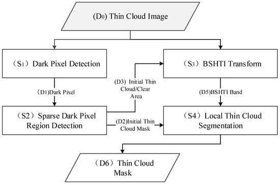
Figure 1.
The flowchart of the proposed method. BSHTI—background suppression haze thickness index.
3.1. Dark Pixel Extraction
For a thin-cloud region, the electromagnetic radiation intensity (e.g., the DN value, reflectance, and the gray level, which we denoted hereafter as the gray level for simplicity) received by the sensor was contaminated by the path radiance. The path radiance increased the observation value for all of the pixels in the thin-cloud area of the remote sensing image, indicating that no dark pixels with extremely low gray levels existed in the visible and near-infrared bands of that area. However, dark pixels in the clear areas of remote sensing images were widely existent and scattered throughout the image. Based on this distinct feature, the thin-cloud area detection problem could be resolved by detecting areas with sparse dark pixels. Consequently, the definition and extraction of dark pixels were crucial to the successful implementation of this algorithm.
In traditional methods, a pixel whose gray value was smaller than the user defined threshold, such as the smallest percent (P) of pixels, was recognized as a dark pixel. However, large areas of shadows, pure water bodies, and dark colored vegetation were often clumped together and formed dark pixel patches, which had a negative effect when measuring the density of dark pixels. To overcome this problem, a dark pixel was defined in a local window (i.e., an area of w × w pixels) to assure the relatively uniform distribution. Accordingly, the dark pixel extraction method was designed as follows:
(1) A cloudy image with n band(s), denoted as , needed to carry out the thin-cloud mask, where represents the ith band of the image. The minimum values of all of the bands were extracted and a new band was formed, which is represented by . For a pixel in the ith row and the jth column, could be expressed by the following equation:
where min represents the minimization operation.
(2) For the band used for , a pixel whose gray level was smaller than the user defined threshold, , was selected as the dark pixel candidate.
is defined using the following formula:
where represents the cumulative histogram of band , and represents the smallest gray level, whose cumulative percentage in is larger than P. The problem for the selection of is transformed to the determination of P, where P indicates a pixel has the potential to become a dark pixel.
As mentioned above, the image content varied; some images contained large portions of dark pixels clumped together; therefore, it was unreasonable to use an identical P for all of the images. Considering this problem, a multiresolution method was utilized in this paper to define the value of P. The image was divided into a group of non-overlapped patches, which were expressed as , where represents a patch with a size of i. To eliminate the negative effects of large areas of dark pixels clumped together, only one pixel in the center of the patches was used to calculate the cumulative histogram.
For the resolution of , the threshold of the dark pixels was determined via Equation (3). Lastly, the final threshold of was obtained by selecting the maximum threshold of all the resolutions:
On this basis for threshold determination, the pixels of were selected as dark pixels candidates.
(3) For a dark pixel candidate along the ith row and jth column, we defined a window surrounding the test pixel with a size of w (i.e., a w × w size). When this pixel was the smallest in the window, it was identified as a dark pixel and flagged with 1; otherwise, it was flagged with 0. The dark pixel bands that were acquired are denoted as :
The dark pixels obtained by this method were defined as feature points, assuming that there were m feature points extracted, which is expressed as follows:
Therefore, only one dark pixel was selected in the local widow to ensure that all these feature points were uniformly distributed with similar densities in the clear areas. However, in the thin-cloud areas, there were either none or only a few dark pixels, which resulted in a low density. Figure 2 shows the dark pixels extracted by the method that was proposed in this study (w = 7, P = 30%). It could be observed that the feature points of the dark pixels had a large quantity and were more uniformly distributed in urban areas and in areas of dense vegetation. By contrast, none or few dark pixels had been found in thin-cloud areas. In other words, dark pixels in these areas were sparse. Depending on the above analysis, thin-cloud detection became a problem when extracting regions where dark pixels were sparse.
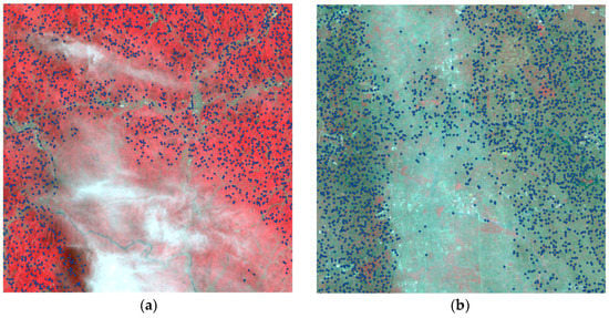
Figure 2.
Dark pixel extraction results for diverse land cover types (w = 7, P = 30%); the blue points represent feature points of dark pixels, where (a) shows the vegetation area, and (b) shows the urban region.
It should be noted that w and P were two essential parameters that decided whether or not a pixel could become a dark pixel, which determined the quantity and distribution of the dark pixels. The parameter set method and its influence on the accuracy of thin-cloud masks will be discussed in detail in Section 5.1.
3.2. Sparse Dark Pixel Region Extraction
Traditionally, point density was mostly measured parametrically based on counting the number of points in a local window. The accuracy obtained by these methods relied on the window shape design and parameters (such as window size), which should be selected carefully. When the feature points were distributed uniformly in a regular shape, all of the approaches could yield favorable results. However, sparse feature point areas formed by thin clouds had irregular shapes, different sizes, and notable differences in their densities. Therefore, it was a challenge to adopt a window-based feature point density measurement, as failure in the effective estimation of sparse feature point densities might have led to the missing detection of thin clouds or a low accuracy of the thin-cloud boundary. To address the problem presented above, a nonparametric point density measurement method was utilized in this study.
The Thiessen polygon was a commonly used zoning method. In the Thiessen polygon result, the distance from any position in the polygon to its corresponding point was shorter than that to any of the other sides of the polygon. Therefore, only one feature point existed within the range of each Thiessen polygon. In other words, a one-to-one corresponding relation existed between the feature points and their Thiessen polygons. Figure 3 shows the Thiessen polygon corresponding to the feature points in Figure 2. It was clear that the area of the polygon was large when the feature points were sparse. According to this fact, a sparse dark pixel region extraction method was designed as follows:
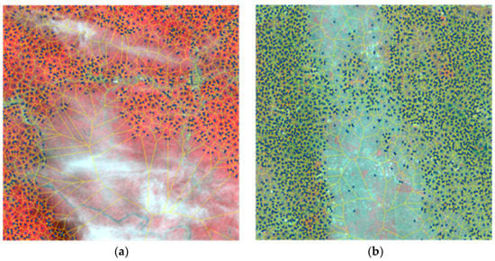
Figure 3.
Schematic diagram of the Thiessen polygon constructed by dark pixels. It can be observed that the area of the Thiessen polygon is small in dense point areas, whereas the area of the Thiessen polygon is large in sparse point areas, where (a) shows the vegetation area, and (b) shows the urban region.
(1) Thiessen polygons, which divided image regions into disjoint subsets, were established according to the feature point set . Then, their areas were calculated and expressed as follows:
where represents the area of the Thiessen polygon corresponding to the feature point, , indicates the density of the feature points around point .
Voronoi diagrams and Thiessen polygons were dual diagrams that interacted with each other, which meant that the Thiessen polygon could be established through the Voronoi diagram. We constructed the Voronoi diagram using a maximum least-angle rule, which could be implemented by multiple classic methods and an improved method.
(2) The Thiessen polygon was divided into two mutually disjoint subsets, which were referred to as the sparse set () and the dense set (). The former represented the sparse areas of feature points, which indicated thin-cloud candidates, and the latter represented their dense areas, which were also known as clear areas. The initial values of and were set as and , respectively. The superscript 0 denoted the number of iterations.
(3) The average and the standard deviation of the polygon for a dense set were calculated using the following formulas:
where represents the number of elements in set .
(4) The large area of the Thiessen polygon indicated the sparse feature points near the location of the feature point. Considering this, polygons satisfying Equation (10) were treated as abnormal values of and were eliminated from the set .
where represents a multiple of the standard deviation, which we set to 3 in this paper. As we selected only one dark pixel in the local window w, whose size was a w × w pixel. Ideally, the area of the Thiessen polygon in the clear part of the image obeyed a normal distribution, whose mean approached the number of w × w pixels. By repeating the experiment with different parameters, = 3 was deemed as appropriate to separate the dense, dark pixel region from the sparse region.
The eliminated polygons were added into set . In this case, two new sets were acquired and denoted as and .
(5) and were utilized as initial values to repeat steps (3) and (4); the iteration process was repeated times until no more polygons met the condition of Equation (10) in set .
(6) The region enclosed by a polygon in the sparse set was recognized as a thin-cloud area candidate. The connected pixels formed a thin-cloud patch and were treated as thin-cloud candidates, which could be expressed as follows:
As certain dark pixels existed near the thin clouds, the candidate thin-cloud area was larger than the real thin-cloud area in most cases, which incurred false detection. Meanwhile, the corresponding detection might have missed some thin clouds with shadows, as an improper area threshold was adopted. Therefore, the boundary of the thin cloud should have been further refined by additional methods.
3.3. BSHTI Transform and Local Segmentation
As a result of the diversity of the land cover and the various thicknesses of thin clouds, it was less likely to represent thin clouds and backgrounds via a unique feature with wide applicability. In addition, single-band segmentation had drawbacks regarding fully exploiting the information contained in the multiband remote sensing image. According to [8], the BSHTI transform, which synthesized the multiband image into a single band, had the capacity to suppress the background and highlight thin clouds. The new band, , obtained by the BSHTI transform, had a linear weighted sum that was calculated by the multiband images. The expression was given as follows:
where represents a series of conversion coefficients for multiple bands.
The objective of this transform was to enable the mean value of the thin-cloud area () in the BSHTI band to be as high as possible, whereas the values in the clear area should have been distributed in a concentrated manner to the greatest extent This meant that the standard variation of the clear area for should have been as small as possible. This problem could be solved by searching for an optimal solution to with a constraint condition of :
The problem could be optimized by the following formula:
where represents the series of conversion coefficients for all of the bands, which was the parameter to be determined. is the correlation coefficient for all of the bands denoted by an matrix. Both and are mean values for all of the bands in the clear and thin-cloud areas, respectively. On the basis of obtaining the value K, could be set to 0 for the convenience of solving .
As a supervised method, thin-cloud and clear areas should have been manually interpreted to calculate the statistics. In this study, candidates of the thin-cloud areas and clear area obtained in Section 3.2 were adopted to train the parameters directly. The conversion results of the image in Figure 2 are presented in Figure 4, which improved the capacity to highlight thin-cloud areas and concentrate various background areas.
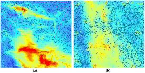
Figure 4.
Schematic diagram of the BSHTI band, the color changing from red to blue indicates the thickness of cloud vary from thick to thin. (a) shows the vegetation area, and (b) shows the urban region.
The false and missing detection of thin-cloud areas might have appeared in regions adjacent to those for candidates of thin-cloud areas. Therefore, thin-cloud areas were iteratively buffered with 1 pixel until the following condition was satisfied:
where refers to the number of pixels additionally found due to buffering, and represents the number of a candidate cloudy area in the pixels. Equation (16) indicated that the proportion of thin clouds to background pixels approached a 1:1 ratio. Then, the Otsu algorithm was employed to define a segmentation threshold for the area of in order to locally separate the thin-cloud area from the clear area. Finally, the thin-cloud mask results were obtained by repeating the morphological operations with a set number of times (in this paper, we set it to four) to remove the rough boundaries and interpolate the missing data.
4. Experiment
4.1. Data and Experimental Method
Multi-spectral images, acquired by sensors of the Wide Field View (WFV) onboard the Chinese Gao Fen 1 (GF1) satellite and the Operational Land Imager (OLI) onboard the Landsat 8 satellite, were utilized to evaluate the performance of the proposed method. Despite minor differences that existed in the spectral channel settings of these sensors, they all contained near-infrared, red, green, and blue bands. The following processing procedures were performed via these four bands. Five images that were acquired by each sensor were selected individually. For simplicity, a subset of size 2000 × 2000 with typical thin-cloud areas and underlying land surfaces was clipped. The meta-information of the test data is shown in Table 1.

Table 1.
The meta-information of the test data; the location is indicated using the image center (i.e., latitude and longitude) for the images acquired by the Wide Field View (WFV) onboard the Gao Fen 1 (GF1) and the path/row in the World Reference System coordinates for images captured by the Operational Land Imager (OLI) onboard the Landsat 8 (L8).
As the images obtained by GF1 WFV and Landsat 8 OLI were characterized with 10-bit and 16-bit resolutions, respectively, all of the bands underwent a linear stretch by means of a percent clip (where the parameter was set to 1%) to force the gray level to remain between 1 and 255. This process might have compressed the gray level of the images and removed the information that was beneficial for separating land covers from thin clouds; better transformation may exist, but for simplicity, this paper utilized a simple, yet acceptable method to normalize the different images. w and P were two important parameters utilized in this experiment. In this paper, w = 7 and P = 30% were used for all of the experiments.
To evaluate the method that was proposed in this study, the results were compared with those via the method that was developed by Makarau et al. [15], which was denoted with the haze thickness map (HTM). In that study, dark pixels were adopted to estimate the haze thickness map, which was similar in principle to that presented in our paper, but with a different implementation method. It was implemented by dividing the images into mutually disjointed windows of definite size to search for the minimum values in all of the windows and use them as dark pixels. By utilizing cubic interpolation, a haze thickness identical to the image resolution could be estimated. Then, the haze was detected using a 21 × 21 window, and the mean value of the haze thickness map was utilized to perform the threshold segmentation for the HTM and define the haze area.
For the ground truth cloud-mask acquisition, the images that were acquired by Landsat 8 OLI were distributed with a Quality Assessment (QA) band, which indicated the pixelwise radiometric quality and included information on cloud confidence, cloud shadow confidence, and cirrus confidence. Since the OLI sensor had a cirrus band, supplemental information was provided to separate thin-cirrus clouds from confusing land covers [20]. In the QA band, two bits were used to indicate the radiometric quality; for example, 00 indicated a non-determined situation, 01 referred to low confidence (0% to 33%), 10 represented medium confidence (34% to 66%), and 11 represented high confidence (67% to 100%). We created a thin-cloud mask with the following rule: cloud or cirrus confidences equal to 11 were assigned as clouds; pixels equal to 10 were assigned as suspected clouds, the remaining conditions were treated as clear pixels.
For the GF1 WFV images, we obtained a ground truth thin-cloud mask via visual interpretation. In terms of substantially thin-cloud images, different interpreters (or the same interpreter at different times) might have generated contradictory thin-cloud interpretation outcomes. Considering this, three interpreters were used in this paper to carry out thin-cloud interpretations and labeled thin clouds independently. The shared areas of these results were selected as the ground truth values of thin clouds. In other words, only thin clouds that were identified by all three interpreters could be seen as thin clouds. Thin clouds that were interpreted by one or two interpreter(s) were recognized as suspected clouds. This interpretation adopted a strategy similar to that of people observe objects from a whole scale to a local scale. First, on a small scale, the entire thin-cloud area was obtained. Then, the images were scaled up to 1:1. In this case, the boundaries of thin-cloud areas were modified to closely fit the boundaries of the thin clouds.
The thin cloud results extracted by our method and the contrasting method were compared with the corresponding ground truth values acquired by the interpreters. In addition, three indexes were acquired: , which represents thin clouds that were correctly detected, , which represents thin clouds that were identified by the algorithm, but with relevant ground truth values that revealed that they were not clouds or thin clouds, and , which refers to thin clouds that were not identified by the algorithm. The unit for these three indexes was a pixel. It is worth noting that the suspected thin clouds could have been classified into thin clouds or clear conditions, without the calculation of false or missing detections. On this basis, the three indexes of true ratio (TR), detection ratio (DR), and overall accuracy (OA) were statistically summarized to evaluate the proposed method in this paper and its contrasting methods. The computational methods are as follows:
4.2. Experimental Results and Performance Evaluation
The thin-cloud mask results via the proposed method and its contrasting methods are illustrated in Figure 5 and Figure 6. In general, our method was able to detect thin clouds with high accuracy and fewer missing data errors. By carefully observing the boundaries between thin clouds and land surface features, we found that the extracted edge adhered to the true edge between the clouds and the clear part of the image. Because our method detected thin clouds within a large range via the Thiessen polygon, and the extraction of thin-cloud areas was based on the buffering of candidate thin-cloud areas, this method was able to effectively avoid confusion regarding high-reflectance surface features, such as small patches of bare soil and buildings. In this way, no salt-and-pepper noise could be generated. It should be noted that sea surfaces or broad water surfaces, which had large amounts of low reflectance dark pixels, combined with an undetermined threshold, detected a certain amount of false dark pixels, which led to the missing detection of thin clouds.
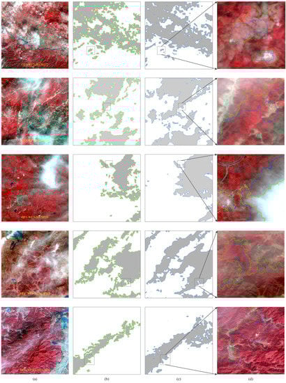
Figure 5.
Thin-cloud mask results of the Wide Field View (WFV) onboard the Gao Fen 1 (GF1). Column (a) is the original image; column (b) shows the cloud mask results using our method; column (c) shows the results from contrasting methods; and column (d) shows the magnified cloud mask results of the local area, where the blue line represents the contrasting results and the green line represents our method’s results.
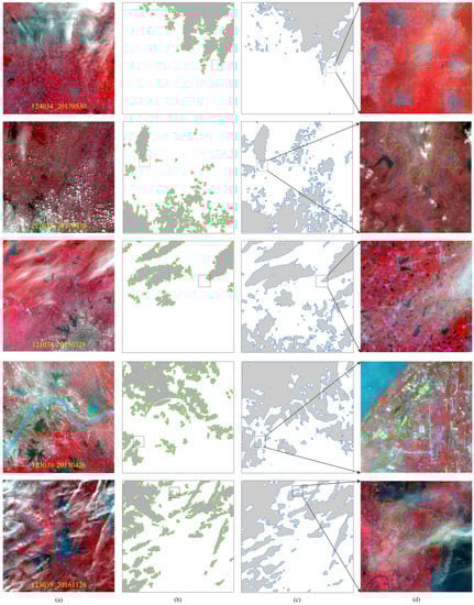
Figure 6.
Thin-cloud mask results of the OLI. Column (a) is the original image; column (b) shows the cloud mask results by our method; column (c) shows the results by contrasting methods; and column (d) shows the magnified cloud mask results of the local area, where the blue line represents the contrasting results and the green line represents our method results.
The HTM used a window to extract dark pixels and estimate the thickness of haze; the large-size thin-cloud detection results were similar to our method. As a result of the influence of window size, however, some missing detection problems could be found in small pieces of the clouds or in thin and long clouds. Similarly, thin-cloud boundaries extracted by the HTM were roughly affected by the window size, and there were mosaic characteristics in the results. Notably, the HTM should have excluded high reflectance objects through the segmentation of buildings and bare soil. Since there were a certain amount dark pixels in urban and bare soil regions, the method proposed in this paper could be adopted to effectively solve confusion regarding high-reflectance surface features, including urban areas.
In Figure 7, we present the statistical metrics of the proposed method and its contrasting methods (TR, DR, and OA). We could observe that the TR average in the proposed method reached 93.22%, and its DR reached 88.7%. Generally, the method proposed in this paper was superior to the HTM method for OA and DR with similar TR values. In addition, the results confirmed that the method could be utilized to perform valid thin-cloud masking for images with medium-spatial resolutions and quantization types. On the basis of removing the pixels influenced by thin clouds and preserving clear pixels to the greatest extent, accurate thin-cloud masks that were acquired by this method could be applied to further thin-cloud removal and land cover-based applications.
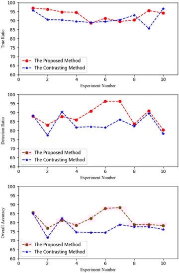
Figure 7.
A comparison between the metrics for the proposed method and those for the contrasting methods.
5. Discussions
5.1. Parameter Setting
The number and distribution of the dark pixels imposed a direct influence on the separation ability of sparse dark pixel areas from the whole image, using threshold segmentation. By determining whether or not a pixel could become a dark pixel, the window size w and the percent threshold P were two key parameters, which should be set carefully by the user. Of these, w represents the size of the local window where a dark pixel exists; P defines the maximum acceptable gray level required by a pixel to become a dark pixel. Excessively low w and large P values could have easily resulted in too many dark pixels; if they were distributed in a thin-cloud area, the corresponding thin area might have been identified as a clear area. On the other hand, when w was too large and P was too small, the number of dark pixels might decrease significantly, resulting in dark pixels that would not be sufficient for separating high-reflectance land surfaces. This caused high reflective land surfaces to be identified as thin clouds.
To evaluate the influence of the parameter setting on the accuracy of the thin-cloud mask, the overall accuracy (OA) of the thin-cloud detection was calculated with a different combination of w and P, where w changed between 7 and 19 with step of 2, and P varied from 5% to 40% with step of 5. Figure 8 shows the OA error bar with changing w and P values; it could be observed that parameter variations within the above range had a minor influence on the OA of the algorithm, as it was simply a tradeoff between the missing detection and the false detection. The results demonstrated that the algorithm was robust over a wide range of parameter settings; therefore, we suggest that the values of w and P could be set to 7 and 30% to obtain an average accuracy with an acceptable true ratio and detection ratio.
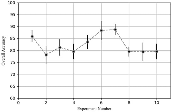
Figure 8.
Overall accuracy variation changes with parameters w (representing the size of the local window where a dark pixel exists) and P (defining the maximum acceptable gray level required by a pixel to become a dark pixel).
5.2. Separation of Thin Clouds from Confusing Land Covers
It was well recognized that thin clouds were often confused with high reflective landscapes, such as urban areas or bright bare soils. As a mixed landscape, urban areas were composed of impervious surfaces (e.g., buildings and roads), vegetation, soil, and waterbodies. Of these, dense vegetation, waterbodies, and shadows of tall buildings and trees could become dark pixels, which were scattered in the urban area around the high reflective pixels in a mosaic pattern. Similarly, a certain number of dark pixels existed in the high reflective bare soil area, such as shadows and low-reflection pixels. The proposed thin-cloud detection method captured the unique features when the portion of thin-clouds in the remote sensing image were mixed with a white component in the visual and near-infrared bands; the result was that no pixels with extremely low values existed in these areas. Since this method detected thin-cloud areas with dark pixels instead of using high reflective values, the problem regarding confusion between high reflective landscapes and thin clouds was resolved. Additionally, the experimental results confirmed that the proposed method possessed the capacity to separate confusing land surfaces from thin clouds. In addition, the method identified thin clouds via local segmentation of the thin-cloud candidate, which suppressed the salt-and-pepper noise that was induced by high reflective landscapes.
As a common approach for thin-cloud detection, this method was robust for both clear images and images composed of clouds. For a clear texture-rich image, where dark pixels were scattered throughout the whole image, the areas of the Thiessen polygons obeyed the normal distribution and were concentrated in the range of the mean, plus or minus three times the standard deviation. Through threshold segmentation of the Thiessen polygon area, few or no sparse dark pixel areas were identified, which caused few or no false detections in the clear texture-rich images. For an image composed of clouds, the dark pixels were sparsely distributed, which exhibited similar features with those in the clear image. However, the minimum gray value or the absolute dark pixel density was larger than that of the clear image, so an additional threshold was required to separate images full of clouds from clear images.
Similar to thin clouds, thick clouds provided missing or distorted landscape information in the remote sensing image. In this respect, there was no need to separate thin clouds from thick clouds. However, semitransparent thin clouds in remote sensing images contained a certain proportion of information about the landscape; then, the thin clouds could be unveiled from the landscape information to obtain a synthetically clear image via an appropriate method (e.g., DOS [2,3], air–light elimination [16], and the fusion based method [17,18]). Since the main objective of our method focused on the identification of the distorted area, there was no clear separation between thin clouds and thick clouds. This method was robust for large, thick clouds. However, this method might have omitted small, thick clouds with corresponding shadows that were distributed near thick clouds.
However, when an image was covered with a large area of waterbody, this method might have failed to mask thin clouds accurately. The spectral signature of clear water was characterized with low reflectance (especially in the near-infrared band) when thin clouds obscure this type of water, and an inappropriate global gray level threshold P. This might have led to the identification of several dark pixels in the thin-cloud area, which resulted in the missing detection problem at the water surface. However, because of the effects of specular reflection and high sediment concentration, several waterbodies were characterized with high- or middle-reflective values, which resulted in none or fewer dark pixels on the smooth and bright water surface. Consequently, false detection could incur.
6. Conclusions
Thin cloud, which is a common radiometric degradation factor in passive remote sensing, reveals land cover information that is lost or distorted in remote sensing images. Accurate thin-cloud masks, which aim to delineate abnormal areas, are critical to guarantee the proper utilization of partially contaminated remote sensing data, which also serve as a precondition for the reconstruction of thin-cloud areas. Conventional thin-cloud mask approaches, which are combined with thin-cloud removal, require a relatively low thin-cloud mask accuracy. To address the problems described above, a thin-cloud mask method based on the sparse dark pixel area extraction has been developed in this paper. This method possesses the following characteristics:
- The scattering effects of thin clouds on solar radiation cause the path radiance to increase in thin-cloud areas, which causes the number of pixels with relatively low values (i.e., dark pixels) in a cloudy area to be much less than those in clear areas. Accordingly, a method has been proposed to extract the candidate of thin-cloud area. Images with diverse backgrounds are used to test this method, and the experimental results indicate that this method is robust under different underlying land covers.
- As a result of the window size setting and the shape selection, traditional template-based approaches may fail to extract thin, long, and small clouds effectively. However, the area of the Thiessen polygon, which is a nonparametric parameter, has been selected to measure the density of dark pixels. Because the Thiessen polygon is constructed with the spatial distribution dark pixels, the area of the Thiessen polygon can measure the density of dark pixels in a nonparametric manner.
- Since dark pixels and brightly colored objects are distributed in a mosaic pattern, conventionally confusing land surfaces, such as high-reflective urban areas and bare soil, can be effectively separated from thin clouds. Additionally, when the final thin-cloud mask is obtained via the local segmentation of the candidate thin cloud, salt-and-pepper noises can also be suppressed.
Although the proposed method is effective for thin-cloud masks compared with the state of art method, it is far from perfect. The false or missing detection of thin clouds also exists, which further restricts the application of data. Improvement of this method is needed to overcome the problems mentioned above.
Acknowledgments
This research is partially supported by the National Key Research and Development Program (Grant No: 2017YFB0503603) and the National Natural Science Fund of China (Grant No: 41631179 and 41301473). The authors are grateful to Imagesky International Co. Ltd. for providing the GF1 image data used in this study. For the investigator’s convenience, we can offer thin-cloud mask for GF1 WFV and Landsat 8 OLI service free of charge for research purposes, if investigators are willing to send us their data to process. Our Email is thuway@163.com.
Author Contributions
Wei Wu developed the thin-cloud mask algorithm and drafted the manuscript. Jiancheng Luo proposed the original idea for the paper. Xiaodong Hu helped conduct the experiment. Haiping Yang and Yingpin Yang gave suggestions to improve the algorithm and experiment, and polished the draft.
Conflicts of Interest
The authors declare no conflict of interest.
References
- Sun, L.; Latifovic, R.; Pouliot, D. Haze Removal Based on a Fully Automated and Improved Haze Optimized Transformation for Landsat Imagery over Land. Remote Sens. 2017, 9, 972. [Google Scholar]
- Zhang, Y.; Guindon, B.; Cihlar, J. An image transform to characterize and compensate for spatial variations in thin cloud contamination of Landsat images. Remote Sens. Environ. 2002, 82, 173–187. [Google Scholar] [CrossRef]
- He, X.; Hu, J.; Chen, W.; Li, X. Haze removal based on advanced haze-optimized transformation (AHOT) for multispectral imagery. Int. J. Remote Sens. 2010, 31, 5331–5348. [Google Scholar] [CrossRef]
- Chen, S.; Chen, X.; Chen, J.; Jia, P.; Cao, X.; Liu, C. An Iterative Haze Optimized Transformation for Automatic Cloud/Haze Detection of Landsat Imagery. IEEE Trans. Geosci. Remote Sens. 2016, 54, 2682–2694. [Google Scholar] [CrossRef]
- Jiang, H.; Lu, N.; Yao, L. A High-Fidelity Haze Removal Method Based on HOT for Visible Remote Sensing Images. Remote Sens. 2016, 8, 844. [Google Scholar] [CrossRef]
- Ancuti, C.O.; Ancuti, C.; Hermans, C.; Bekaert, P. A fast semi-inverse approach to detect and remove the haze from a single image. In Asian Conference on Computer Vision; Springer: Berlin/Heidelberg, Germany, 2010; Volume 6, pp. 501–514. [Google Scholar]
- Kauth, R.J.; Thomas, G.S. The Tasselled Cap—A Graphic Description of the Spectral-Temporal Development of Agricultural Crops as Seen by Landsat. LARS Symposia. 1976. Available online: docs.lib.purdue.edu/cgi/viewcontent.cgi?article=1160&context=lars_symp (accessed on 13 April 2018).
- Crist, E.P.; Cicone, R.C. A physically-based transformation of Thematic Mapper data—The TM Tasseled Cap. IEEE Trans. Geosci. Remote Sens. 1984, 3, 256–263. [Google Scholar] [CrossRef]
- Liu, C.; Hu, J.; Lin, Y.; Wu, S.; Huang, W. Haze detection, perfection and removal for high spatial resolution satellite imagery. Int. J. Remote Sens. 2011, 32, 8685–8697. [Google Scholar] [CrossRef]
- Fries, R.; Modestino, J. Image enhancement by stochastic homomorphic filtering. IEEE Trans. Acoust. Speech Signal Process. 1979, 27, 625–637. [Google Scholar] [CrossRef]
- Shen, H.; Li, H.; Qian, Y.; Zhang, L.; Yuan, Q. An effective thin cloud removal procedure for visible remote sensing images. ISPRS J. Photogramm. 2014, 96, 224–235. [Google Scholar] [CrossRef]
- Wu, C.; Wang, Q.; Yang, Z. Cloud-moving of Water RS Image Based on Mixed Pixel Model. J. Remote Sens. 2006, 10, 176–182. (In Chinese) [Google Scholar]
- He, K.; Sun, J.; Tang, X. Single image haze removal using dark channel prior. IEEE Trans. Pattern Anal. Mach. Intell. 2011, 33, 2341–2353. [Google Scholar] [PubMed]
- Vermote, E.F.; Tanré, D.; Deuze, J.L.; Herman, M.; Morcette, J.J. Second simulation of the satellite signal in the solar spectrum, 6S: An overview. IEEE Trans. Geosci. Remote Sens. 1997, 35, 675–686. [Google Scholar] [CrossRef]
- Makarau, A.; Richter, R.; Mller, R.; Reinartz, P. Haze Detection and Removal in Remotely Sensed Multispectral Imagery. IEEE Trans. Geosci. Remote Sens. 2014, 52, 5895–5905. [Google Scholar] [CrossRef]
- Fattal, R. Single image dehazing. ACM Trans. Graph. (TOG) 2008, 27, 72. [Google Scholar] [CrossRef]
- Schaul, L.; Fredembach, C.; Süsstrunk, S. Color image dehazing using the near-infrared. In Proceedings of the 16th IEEE International Conference on. Image Processing (ICIP), Cairo, Egypt, 7–10 November 2009; pp. 1629–1632. [Google Scholar]
- Ancuti, C.; Ancuti, C.O.; De Vleeschouwer, C.; Bovik, A.C. Night-time dehazing by fusion. In Proceedings of the 2016 IEEE International Conference on Image Processing (ICIP), Phoenix, AZ, USA, 25–28 September 2016; pp. 2256–2260. [Google Scholar]
- Chavez, J. An improved dark-object subtraction technique for atmospheric scattering correction of multispectral data. Remote Sens. Environ. 1988, 24, 459–479. [Google Scholar] [CrossRef]
- Gao, B.C.; Li, R.R. Removal of Thin Cirrus Scattering Effects in Landsat 8 OLI Images Using the Cirrus Detecting Channel. Remote Sens. 2017, 9, 834. [Google Scholar] [CrossRef]


© 2018 by the authors. Licensee MDPI, Basel, Switzerland. This article is an open access article distributed under the terms and conditions of the Creative Commons Attribution (CC BY) license (http://creativecommons.org/licenses/by/4.0/).