Abstract
Clouds remain one of the largest sources of uncertainty in remote sensing of surface temperature in the infrared, but this uncertainty has not generally been quantified. We present a new approach to do so, applied here to the Advanced Along-Track Scanning Radiometer (AATSR). We use an ensemble of cloud masks based on independent methodologies to investigate the magnitude of cloud detection uncertainties in area-average Land Surface Temperature (LST) retrieval. We find that at a grid resolution of 625 km (commensurate with a 0.25 grid size at the tropics), cloud detection uncertainties are positively correlated with cloud-cover fraction in the cell and are larger during the day than at night. Daytime cloud detection uncertainties range between 2.5 K for clear-sky fractions of 10–20% and 1.03 K for clear-sky fractions of 90–100%. Corresponding night-time uncertainties are 1.6 K and 0.38 K, respectively. Cloud detection uncertainty shows a weaker positive correlation with the number of biomes present within a grid cell, used as a measure of heterogeneity in the background against which the cloud detection must operate (e.g., surface temperature, emissivity and reflectance). Uncertainty due to cloud detection errors is strongly dependent on the dominant land cover classification. We find cloud detection uncertainties of a magnitude of 1.95 K over permanent snow and ice, 1.2 K over open forest, 0.9–1 K over bare soils and 0.09 K over mosaic cropland, for a standardised clear-sky fraction of 74.2%. As the uncertainties arising from cloud detection errors are of a significant magnitude for many surface types and spatially heterogeneous where land classification varies rapidly, LST data producers are encouraged to quantify cloud-related uncertainties in gridded products.
1. Introduction
All geophysical variables are retrieved with a level of uncertainty, which is a function of both the data used and the retrieval methods. Taking account of uncertainty is fundamental to the appropriate scientific application of these data, and uncertainty information should be provided in the most complete state possible by data producers, preferably for each datum where uncertainty varies sufficiently to justify this [1]. Within the surface temperature remote sensing community, there have been recent efforts to quantify measurement uncertainties on a per-pixel basis. This has been achieved either by developing a model of how uncertainties vary under different retrieval conditions [2,3] or by estimating uncertainties within the retrieval process itself [4,5]. In the latter case, the uncertainties can be validated in addition to the measurement data, using independent reference datasets [6].
A method for estimating per-pixel uncertainty in sea surface temperature retrieval was developed within the context of the European Space Agency (ESA) Climate Change Initiative (CCI) programme [4]. It has since been adopted within the lake surface temperature community via the European Commission EU Surface Temperature of All Corners of Earth (EUSTACE) project, and within the land surface temperature (LST) community via the ESA Data User Element (DUE) GlobTemperature project [5,7]. These data producers consider the propagation of uncertainties arising from random and systematic errors from Level 1b data into Level 2 and Level 3 products. The investment of these different data producers in using the same approach to characterise uncertainty in surface temperature retrievals is an important step in providing comparable products across different domains (land, ocean, lake, ice).
The uncertainties currently characterised by these data producers include both random and systematic components. Sources of uncorrelated (random) errors in land surface temperature data include instrument noise and sampling uncertainties. Systematic uncertainties arise due to retrieving surface temperature through the atmosphere, sub-pixel variability in emissivity and from calibration and instrument characteristics that change over time. Surface temperature retrievals are predominantly made using measurements in the infrared region of the electromagnetic spectrum and are therefore affected by the presence of clouds. Sampling uncertainties due to the presence of cloud limiting the observations available in gridded data have been considered in sea surface temperature products [8], but uncertainties due to imperfect cloud screening impacting the retrieved surface temperature have not previously been quantified.
Cloud detection is an essential pre-processing step in the retrieval of Earth surface temperatures, as cloud will affect the observed brightness temperatures. Clouds are the source of two different types of uncertainty in surface temperature retrieval: (1) uncertainty due to ‘missed clouds’ (errors of omission), which typically result in a cold bias in the retrieved surface temperature; and (2) uncertainty due to ‘missed measurements’ (errors of commission), resulting from clear-sky pixels falsely classified as cloud. At Level 2, (2) simply leads to omission of valid data from a given dataset, but at Level 3, this has an impact on the averaged surface temperatures within a given gridded domain, not explicitly accounted for within the sampling uncertainty. Where clouds are missed (1), uncertainties may also include errors arising from the application of a clear-sky infrared LST retrieval algorithm to cloud-affected observations.
Cloud detection algorithms predominantly work on the concept that clouds are ‘bright’ in the visible part of the spectrum and ‘cold’ in the infrared part of the spectrum. Cloud screening techniques range from threshold-based testing [9,10,11], to neural networks [12,13,14,15], probabilistic approaches [16,17] and full Bayesian probability calculations [18]. Problems typically occur where the clouds are of a similar temperature to the underlying surface (e.g., low-level fog), along clear-cloud transition zones and over bright and/or cold surfaces [19,20,21,22]. At night, visual detection efficiency is reduced, amplifying the challenge of detecting low-level warm clouds. Detection difficulties can also be magnified over land due to rapid spatial variations in land surface emissivity and surface reflectance, making retrievals more difficult over pixels containing multiple land surface types and varying surface topography [17,23,24].
Cloud detection errors contribute to structural uncertainty in surface temperature retrieval, an uncertainty arising due to the methodological approaches adopted in the retrieval (e.g., which type of cloud detection algorithm is used) [25]. Quantifying structural uncertainties in remotely-sensed LST due to cloud detection failures is challenging without a ‘truth’ mask against which to make comparisons, and will of course be dependent on the cloud masking technique chosen in the creation of any given data product. There is an awareness within the remote sensing community that cloud mask failures do impact retrieval uncertainty [2,26], but the magnitude of cloud detection uncertainties in LST retrieval have yet to be fully quantified. In this paper, we use data from multiple cloud masks collated within a cloud detection inter-comparison exercise for the Advanced Along-Track Scanning Radiometer (AATSR), within the European Space Agency (ESA) Data User Element (DUE) GlobTemperature project. Collating a range of leading cloud masks over a consistent set of images enables us to evaluate structural uncertainties due to clouds using an ensemble approach. Multiple independent datasets help to resolve the state-space of the structural uncertainty [25] and provide an estimate of its magnitude. The paper proceeds as follows: we describe the cloud clearing inter-comparison (Section 2), our approach to deriving LST uncertainties within the retrieval process (Section 3) and our understanding of cloud masking uncertainties using the ensemble data (Section 4). We present the discussion and conclusions in Section 5.
2. Cloud Clearing Inter-Comparison
The cloud clearing inter-comparison within the ESA DUE GlobTemperature project was designed to assess a range of different cloud detection techniques for their suitability in land surface temperature (LST) retrieval from the Advanced Along-Track Scanning Radiometer (AATSR). AATSR, the third in a series of such instruments (following ATSR-1 and ATSR-2), flew aboard Envisat and was the precursor to the now operational Sea and Land Surface Radiometer (SLSTR) aboard Sentinel-3. This instrument series was designed specifically for the retrieval of surface temperature and is therefore the optimal choice for the production of a long-term LST climate data record (CDR) [27].
AASTR is a dual-view radiometer, making observations at 1-km resolution at the sub-satellite point in the nadir view (with viewing angles of 0–22) and a second observation in the forward view (with viewing angles of 52–56). AATSR has seven channels covering the visible and infrared spectrum, centred at 0.55, 0.66, 0.87, 1.6, 3.7, 10.8 and 12 m. It flew between 2002 and 2012 in Sun-synchronous orbit with an Equator overpass time of 10.30 a.m. For LST retrieval, only observations in the nadir view are used.
The cloud-clearing inter-comparison exercise had three phases designed to give participants an opportunity to develop their algorithms prior to the final comparison: training, testing and submission. At each stage, data for ten AATSR sub-scenes were provided, with a size of 512 × 512 pixels. These scenes were chosen to cover a wide range of conditions, specifically focussing on those where cloud detection is known to be more challenging. Within each set of ten scenes, as many as possible of the following conditions were represented: cumulus, stratus and cirrus cloud types; desert, vegetated, forest, ice and coast land surface types; a range of atmospheric total column water vapour (TCWV) and scenes where some dust or smoke aerosol was present. The training phase was designed for algorithm development, and the test dataset was available to ensure that developers had not tuned their algorithm too closely to a particular scene selection. At these stages, a ‘truth’ cloud mask was created manually by expert inspection and provided to algorithm developers to assess their cloud mask performance. The analysis in this paper uses the final submission dataset where participants provided their data ‘blind’ without reference to a truth cloud mask (although this was available at the point of analysing the ensemble). A full description of the submission scenes is provided in Table 1.

Table 1.
Key characteristics of the ten submission scenes used within the cloud clearing inter-comparison.
Figure 1 shows the 10.8-m brightness temperatures for each of the ten scenes at native resolution (∼1 km). Particular features to note are that Scene 3 contains a fire with some smoke aerosol in the top right quadrant of the image, but the spatial extent of high aerosol loading is limited. Scene 5 has a significant dust aerosol loading across the bottom-right of the image, which will affect the LST where a retrieval is made. Scene 7 is a composite of ice over land and sea-ice with some cloud cover over the left side of the peninsula ridge and towards the top of the image. LST is only retrieved over the Antarctic Peninsula and not over the sea-ice region (GT_ATS_2P v1.0 dataset).
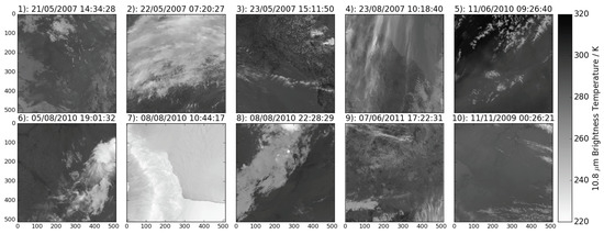
Figure 1.
The 10.8-m brightness temperatures for the 10 submission scenes in the cloud clearing inter-comparison (Table 1) at native resolution (∼1 km). Individual plot headings give the scene number, date and orbit start time.
The data provided to algorithm developers with each scene were designed to be comprehensive enough to implement any type of cloud detection scheme. Observations were provided for collocated views (forward and nadir) in all channels, in addition to the land-sea mask, and confidence flags from the L1b data. Numerical weather prediction (NWP) data were provided for those algorithms dependent on radiative transfer simulation, including skin temperature and TCWV from ERA-Interim data [28], and surface emissivity and reflectance from the UVIREMIS and BRDF atlases [29,30]. These are used as inputs into the RTTOV 11 fast radiative transfer model [31] to simulate top of atmosphere reflectance and brightness temperatures. We also supplied land surface cover data, which is a variant of the GlobCover dataset [5] and all-sky LST (i.e., with no cloud detection pre-processing).
Expert cloud masks were generated for each of the 30 scenes across the three phases of the inter-comparison exercise. These were constructed using a bespoke tool developed for this purpose by the Institute for Environmental Analytics at the University of Reading [32]. It enables the user to view a given scene from a number of different instrument channels concurrently and to easily construct channel inter-comparisons (such as differences, RGB images and local standard deviations). The majority of cloud in a given scene can generally be masked using thresholds on the channel data specific to the image (set using sliders), and in challenging regions, the mask can be edited by hand. This allows the user to refine the masking in areas such as cloud edges and sunglint where thresholds appropriate for the majority of the image may not apply locally. Figure 2 shows this manual cloud mask for each of the scenes in the submission dataset for land only (ocean and inland water bodies are masked out and shown in blue). The classification tool allowed pixels to be classified as ‘clear’, ‘probably clear’, ‘probably cloud’ and ‘cloud’. ‘Clear’ and ‘cloud’ were the most commonly-used categories, with ‘probably clear’ and ‘probably cloud’ used infrequently, typically in the proximity of aerosol. For analysis purposes, the few ‘probably clear’ pixels are interpreted as clear-sky and ‘probably cloud’ pixels interpreted as cloud. The dust aerosol in Scene 5 is set as clear-sky by the manual mask for the purpose of considering cloud masking uncertainties, but aerosol with a high optical depth will also affect the retrieved LST.
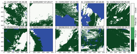
Figure 2.
Manual cloud mask for the 10 submission scenes in the cloud clearing inter-comparison (Table 1) at native resolution (∼1 km). Individual plot headings give the scene number, date and orbit start time. Ocean and inland water bodies are plotted in blue.
There were eight participants in the cloud clearing inter-comparison from across Europe, including the AATSR operational cloud mask from the Synthesis of ATSR Data Into Sea-Surface Temperature (SADIST) [9], the AATSR Dual View V2 (ADV V2) [11,33], the Avhrr Processing scheme Over Land, cLouds and Ocean- Next Generation (APOLLO_NG) [16], Optimal Retrieval of Aerosol and Cloud (ORAC) [10], Generalised Bayesian Cloud Screening (Bayes Min and Bayes Max) [17,18], Community Cloud Retrieval for Climate (CC4CL) [14,15] and the University of Leicester Version 3 (UoL_V3) [17,34] algorithms. This selection of algorithms represents a wide range of cloud detection techniques, including threshold-based testing, neural networks, probabilistic approaches and full Bayesian calculations. With the exception of SADIST, the algorithms have all been developed within the following European Space Agency-funded projects: GlobTemperature Data User Element, Long-Term Land Surface Temperature Validation, Aerosol Climate Change Initiative (Aerosol_cci) and Cloud CCI; and have a wider use within the Earth Observation community beyond the extensive datasets produced within these projects. Full details on each of the contributing algorithms are provided in Table 2. Subsequent to the time of submission to the cloud clearing inter-comparison exercise, the ORAC algorithm has been replaced by the CC4CL algorithm within Aerosol_cci and is not therefore included in the ensemble analyses presented in this paper.
Table 2.
Key characteristics of the cloud detection algorithms submitted to the GlobTemperature Cloud Clearing Inter-Comparison exercise. Expansion of algorithm acronyms are as follows: Synthesis of ATSR Data Into Sea-Surface Temperature (SADIST); AATSR Dual View V2 (ADV 2); the Avhrr Processing scheme Over Land, cLouds and Ocean-Next Generation (APOLLO_NG); Optimal Retrieval of Aerosol and Cloud (ORAC); Bayesian Cloud Detection (Bayes Min and Bayes Max); Community Cloud Retrieval for Climate (CC4CL); University of Leicester Version 3 (UoL_V3).
3. Uncertainties in LST Retrieval
LST from AATSR is retrieved using the 10.8 and 12 m channels in a nadir-only split window algorithm [5,35].
where a, b and c are retrieval coefficients, dependent on biome (i), fractional vegetation cover (f), precipitable water (pw) and satellite viewing angle (p()). T and T denote the 10.8 and 12 m brightness temperatures, respectively. The retrieval coefficients vary as a function of time of day (day or night), and the dependent parameters vary on differing length scales: the biome or land cover classification is fixed for a given location throughout time, whilst the precipitable water and fractional vegetation cover change seasonally. The land cover classification is based on the GlobCover dataset [36], regridded at 1/120 resolution. The bare soil category is sub-divided into six different classes, giving a total of twenty-seven distinct land cover classifications. Fractional vegetation cover is calculated from the Copernicus Global Land Services dataset [37] at ten-day temporal resolution, whilst the precipitable water is derived from the six-hourly ERA-Interim dataset [28].
Uncertainties in the LST retrieval arise from instrument noise, instrument calibration, specification of surface parameters (e.g., surface emissivity, land cover classification) and because the retrieval is made through the Earth’s atmosphere. Radiative transfer is simulated in the retrieval process using a fast forward model (RTTOV 11) constrained by Numerical Weather Prediction (NWP) data. Uncertainties are characterised using an approach consistent with the production of sea surface temperature data within the ESA CCI project [4,8], where an uncertainty budget is constructed from a number of distinct components: uncorrelated, locally correlated and systematic uncertainties [5]. Random errors are those that have no correlation between observations and include instrument noise and sub-pixel variability in surface emissivity not captured by the auxiliary data. Locally systematic uncertainties arise from errors in the surface emissivity for different land cover classifications (captured implicitly in the fractional vegetation cover), errors in the atmospheric state (via the precipitable water and radiative transfer parametrisations), errors in the selection of retrieval coefficients, errors in geolocation and uncertainty in the knowledge of the underlying biome. Within the retrieval, these locally systematic uncertainties are considered as two separate components relating to the surface (sfc) and atmosphere (atm). Finally, the large-scale systematic uncertainty arises from calibration errors and the bias in the satellite surface temperatures relative to other sources of temperature data, once all known residual biases are corrected for [38]. This is currently set to a fixed value of 0.03 K [5]. Although the magnitude of individual uncertainty components can be algorithm dependent, the total uncertainty budget tends to be similar across different LST retrieval schemes.
Within this paper, we consider uncertainties in the LST data when gridded at a 25 × 25 pixel resolution corresponding to a surface area of 625 km. This is commensurate with a gridded resolution of 0.25 at the tropics, a typical grid size for global surface temperature products. At Level 3, an additional source of uncertainty is introduced via the gridding process as LST can only be retrieved for clear-sky pixels. The sampling uncertainty () is calculated as follows:
where n is the number of cloudy pixels in the grid cell, n is the number of land pixels in the grid cell and is the standard deviation of the LST across the clear-sky pixels in the grid cell. Where there is only a single clear-sky pixel in the grid cell (and the LST standard deviation cannot be calculated), the variance is set to the maximum value across the scene. The sampling uncertainty is uncorrelated between Level 3 grid cells and is added to the upscaled Level 2 random uncertainty, where and denote the Level 2 and Level 3 random uncertainty components, respectively.
The subscript ‘clr’ denotes clear sky pixels over land within the 625 km grid cell. The Level 2 atmospheric uncertainty component () is upscaled to Level 3 () as follows, assuming that atmospheric state effects are correlated over length scales of 25 km:
For the surface component, it is assumed that the uncertainties are correlated with a length scale of 5 km, consistent with the resolution of the auxiliary surface datasets, but are uncorrelated over larger spatial scales. The AATSR data are at a native resolution of 1 km, so to calculate the Level 3 surface uncertainty component (), we first calculate an intermediate surface uncertainty component at 25 km () before upscaling this to 625-km resolution.
The total uncertainty in a grid cell () is given by adding all of the Level 3 uncertainty components in quadrature.
where the Level 3 large-scale systematic uncertainty () is equal to 0.03 K as this is fully correlated across the gridded domain. The retrieval uncertainties (not including cloud detection uncertainties) for the ten scenes in the cloud clearing inter-comparison are shown in Figure 3. They are calculated having applied the manual cloud mask to the data, and the uncertainties are set to zero for entirely cloudy grid cells. We see that typically, the minimum retrieval uncertainty at this resolution is ∼1 K, increasing in some regions to 2–3 K. This is particularly evident over Florida (Scene 3), across parts of the U.K. (Scene 4), over Uruguay (Scene 5) and across Mauritania (Scene 9).
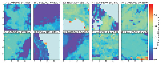
Figure 3.
Level 3 LST retrieval uncertainties for the 10 submission scenes in the cloud clearing inter-comparison (Table 1) at 625-km resolution. Individual plot headings give the scene number, date and orbit start time.
We calculate a cloud masking uncertainty for these ten scenes using the ensemble of contributing cloud masks. Seven masks are applicable during the day and only five at night (as ADV and APOLLO_NG were designed for daytime classification only). We apply each cloud mask to the unfiltered LST field in turn and calculate an average LST in each 625-km grid cell. We then calculate the LST difference between applying the manual mask (MM) in each grid cell and applying each of the contributed masks (CM) in turn (). The cloud masking structural uncertainty is then the standard deviation of the ensemble of LST differences. We classify any grid cells with 600 or more pixels with an ocean biome (out of 625 pixels in a given grid cell) as water and do not consider them in this analysis. For any land grid cells, the lower threshold on the number of clear-sky pixels required to calculate the mean LST is one, as this methodology is applied in the generation of operational products. Figure 4 shows the cloud masking uncertainties for each of the ten scenes. The magnitude of the cloud masking uncertainty is 0 K where all masks (including the manual mask) agree that there is clear-sky, and grid cells where all masks agree that it is cloudy are shown in white. Cloud masking uncertainties over largely clear regions range between 0 and 0.5 K. Small variations in the pixels flagged as cloud within a given grid cell will cause some uncertainty in the retrieved LST, as this is not homogeneous at 1-km resolution. Cloud masking uncertainty typically increases around the edges of cloud features and some land features where one or more masks incorrectly interpret them as cloud, being of the order of 1.5–3 K in magnitude. There is also some evidence of increased cloud detection uncertainty over broken cloud fields (Scenes 3 and 9). In some regions, the cloud masking uncertainty increases significantly to >10 K, and this uncertainty has higher spatial variability than the LST retrieval uncertainty. Figure 5 shows the retrieval (Equation (7)) and cloud masking uncertainties added in quadrature. The spatial variability from the cloud masking uncertainty dominates, with minimum total uncertainties typically of the order 1.5 K in clear-sky regions. Regions of large cloud masking uncertainty do not always correlate with regions of high retrieval uncertainty, for example over the U.K. (Scene 4) and Mauritania (Scene 9).
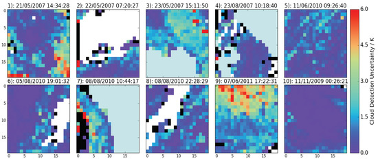
Figure 4.
Cloud detection uncertainties for the 10 submission scenes in the cloud clearing inter-comparison (Table 1 and Table 2) at 625-km resolution. Individual plot headings give the scene number, date and orbit start time. White grid cells denote agreement between all masks on cloudy conditions. Black grid cells denote regions classified as entirely cloudy by the manual mask, but clear-sky in some of the contributing masks.
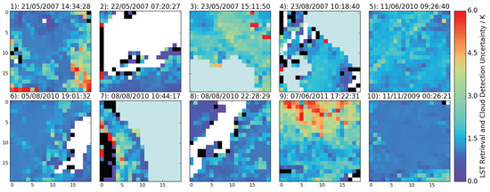
Figure 5.
Combined Level 3 LST retrieval and cloud detection uncertainties for the 10 submission scenes in the cloud clearing inter-comparison (Figure 3 and Figure 4) at 625-km resolution. Individual plot headings give the scene number, date and orbit start time. White grid cells denote agreement between all masks on cloudy conditions. Black grid cells denote regions classified as entirely cloudy by the manual mask, but clear-sky in some of the contributing masks.
4. Understanding Cloud Detection Uncertainties
Cloud detection uncertainty shows some spatial correlation with the location of cloudy features (Figure 2), but also has a spatial variability related to the land surface cover. We would expect cloud detection uncertainty to be positively correlated with the cloud fraction. Where fewer clear-sky pixels are available, these are less likely to be representative of the gridded mean LST, as the per-pixel values generally show a degree of heterogeneity. The spatial variability related to land surface cover is driven by several factors affecting the individual cloud masks within the ensemble: (1) Some cloud masks, particularly the threshold based methods, are sensitive to land features such as riverbeds. It is very difficult to select globally-applicable thresholds for cloud detection tests, and inevitably, those chosen work better in some regions than in others. Erroneous flagging of surface features will generate discrepancies in the mean LST between different cloud masks, increasing the cloud detection uncertainty. (2) The variability in the land cover classification within a given grid cell is also important. Where the land surface biome has a large variability, the LST is likely to vary more rapidly spatially, and the difference in sub-sampling of the cell introduced by the different cloud detection schemes (i.e., variations in the definition of the cloud edge) will have a more significant impact. In this situation, the spread of differences in LST with respect to the manual cloud mask will increase. Under these conditions, the distribution of different biomes within a grid cell will also be important, e.g., with a steady gradient in LST across the grid cell potentially giving a different uncertainty to a more heterogeneous LST field. Assuming a perfect cloud mask under these conditions, sampling uncertainties would also be higher here, than in more homogeneous regions [8].
Given these factors, it may be expected that we can parametrise Level 3 uncertainties as: (1) a function of the percentage of clear-sky pixels within a grid cell and (2) as a function of the underlying variability in LST. We examine both, using the manual mask as ‘truth’ for the percentage of clear-sky pixels, and the number of land biomes within a given grid cell as a proxy for LST variability, as we do not have representative LST’s for cloudy pixels.
Figure 6 shows the number of clear-sky pixels in each 625-km grid cell. Comparing this with Figure 4, we see some spatial correlations between lower percentages of clear-sky pixels and high cloud detection uncertainties, notably around the cloud features over China (Scene 1), Russia (Scene 2), Algeria (Scene 6) and in the top half of the Mauritania image (Scene 9). We also see regions where larger cloud detection uncertainties do not correspond to lower clear-sky percentages, for example over Canada (Scene 10, to the left of the image) and over the Antarctic Peninsula (Scene 7). Figure 7 shows the number of biomes in each 625-km grid cell for each scene. Here, we see that the number of biomes correlates positively with cloud detection uncertainty over China (Scene 1, to the right of the image) and over Florida (Scene 3).
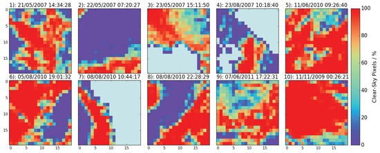
Figure 6.
Clear-sky fraction for the 10 submission scenes in the cloud clearing inter-comparison (Table 1) at 625-km resolution. Individual plot headings give the scene number, date and orbit start time.
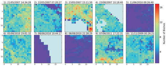
Figure 7.
Number of land biomes for the 10 submission scenes in the cloud clearing inter-comparison (Table 1) at 625-km resolution. Individual plot headings give the scene number, date and orbit start time.
We examine the relationship between cloud detection uncertainty and the percentage of clear-sky pixels as defined by the manual mask across the ten scenes, excluding Scene 5 (high dust aerosol loading) and Scene 7 (Antarctic Peninsula). These data are excluded for the following reasons: (1) firstly because aerosol affects the retrieved LST, and the most appropriate treatment of aerosol affected pixels is dependent on the data application (see the discussion section for further details); (2) secondly because most cloud detection algorithms show very poor skill over ice, tending to flag all ice as cloud, or on occasion all ice as clear-sky, but failing to discriminate well between snow or ice surfaces and cloud. The cloud detection uncertainties in these particularly challenging regions are considered further at the end of this section.
Figure 8a shows the relationship between the percentage of clear-sky pixels over land and the cloud detection uncertainty at 625-km resolution. The percentage of clear-sky pixel data on the x-axis is binned in 10% increments, and panel (b) shows the number of grid cells in each bin. The cloud detection uncertainty is the mean value across all grid cells in a given bin, and the error bars represent the standard error. The solid line shows all of the data from the eight scenes (excluding Scenes 5 and 7), indicating a negative correlation between the percentage of clear-sky pixels and cloud detection uncertainty. For a 10–20% clear-sky fraction, we see average cloud detection uncertainties of 2 K, which fall to 0.65 K for a clear-sky fraction between 90 and 100%.
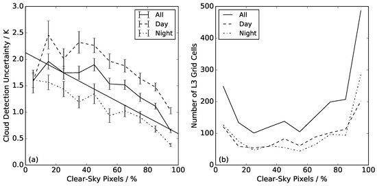
Figure 8.
Cloud detection uncertainties as a function of clear-sky fraction (a) at 625-km resolution. The following are shown: all data (solid line), night-time only (dot-dash line) and daytime only (dashed line). The linear regression for cloud detection uncertainty as a function of clear-sky percentages is shown for all data. Panel (b) shows the number of observations in each bin.
Of the scenes included in the analysis, four are daytime observations and four night-time observations, and we calculate the cloud detection uncertainty under these conditions independently. We see from the number of grid cells that this still gives ≥50 observations within each bin under different solar illuminations. The cloud detection uncertainties during the day are of larger magnitude than at night, but the slope of the relationship between uncertainty and clear-sky fraction is consistent with that shown for all of the data. At clear-sky fractions of 10–20%, cloud detection uncertainties are on average 2.5 K during the day and 1.6 K at night, falling to 1 K and 0.38 K respectively for clear-sky fractions of 90–100%. The magnitude of the day-night difference in cloud detection uncertainties for any given clear-sky fraction is of the order 0.6–0.8 K. We would not expect the cloud detection uncertainties to be 0 K at 100% clear-sky as this definition is applicable to the manual mask only.
We also consider the cloud detection uncertainty as a function of the number of biomes present in the Level 3 grid cell, as a measure of the heterogeneity in the background against which the cloud detection must operate, e.g., surface temperature, emissivity and reflectance (Figure 9). We present results for grid cells with between four and twelve different biomes as this is the typical range for the majority of observations. Again, we plot all data and then day and night-time observations independently. We find a general increase in the cloud detection uncertainty with the number of biomes, although the relationship is not as consistent as that found with the clear-sky fraction. There will be a dependence on the biome type that folds into this analysis. For example, if all the biomes are different types of forest vegetation, the LST variability will be much lower than where the biome set includes more diverse biome types, e.g., bare soil and forest. At night, there seems to be a stronger relationship between the cloud detection uncertainty and the number of biomes and a much weaker one during the day. There is a time of day-dependent difference in cloud detection uncertainty where the number of biomes is few: 0.5 K at night and 1.5 K during the day for four biomes. For 11–12 biomes in a given grid cell, we see convergence in the uncertainties, which are typically of order 1.7 K under all conditions (for 11 biomes per grid cell).
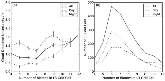
Figure 9.
Cloud detection uncertainties as a function of number of biomes in each grid cell (a) at 625-km resolution. The following are shown: all data (solid line), night-time only (dot-dash line) and daytime only (dashed line). Panel (b) shows the number of observations in each bin.
Finally, we examine whether this dataset can reveal any differences in the cloud detection uncertainties under different land cover classifications. To do this, we consider all ten scenes and look for grid cells that have a dominant biome, defined as where 80% or more of the land pixels within the grid cell have a single land cover classification. Within our scenes, we found five biomes for which we had 40+ grid cells in which they were the dominant land cover, as shown in Table 3. For each land cover classification considered here, the observations had a range of clear-sky fractions, upon which cloud detection uncertainty has a significant dependence (as shown in Figure 8). We therefore standardise all the results to the average percentage of clear-sky pixels across the five biomes (74.2%). We compare the model slope from a linear regression of all data against the clear-sky fraction (Figure 8) against the linear regressions of data points falling within each of the five identified biomes. We find that the slope of the model is strongly biome dependent (Figure 10a) and that a biome-specific correction to a clear-sky fraction of 74.2% is required. The linear regression gives each data point an equal weighting, with the assumption that we have the same confidence in the cloud detection uncertainty at every location, in the absence of any other information. The uncertainty in the regression model is calculated as the standard deviation of the statistical differences between the model and the data points (Table 3). The mosaic vegetation has the best constrained fit with a standard deviation in the model-data differences of 0.11 K. For bare soils, the standard deviation is ∼0.34 K, for forests 0.57 K and for permanent snow and ice 1 K. This means that there is a greater uncertainty in the regression model for forest and permanent snow and ice classes.
Table 3.
Land cover classification numbers, descriptions, number of observations and regression model uncertainties corresponding to the data shown in Figure 10.
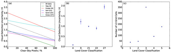
Figure 10.
Biome-specific linear regression models for cloud detection uncertainty dependence on clear-sky fraction (a). Standardised cloud detection uncertainties as a function of land cover classification (b). Panel (c) shows the number of observations for each land cover classification, with land cover classifications defined in Table 3.
Figure 10 shows relative cloud detection uncertainties between the biomes. Panel (b) shows the mean standardised cloud detection uncertainty at 74.2% clear-sky fraction plotted for each biome, including the standard error on the mean (note that the absolute magnitude of these will vary with clear-sky fraction). Panel (c) shows the number of observations available for each land cover classification. We see here that the magnitude of the cloud detection uncertainty shows a significant dependence on the underlying biome. The largest cloud detection uncertainties are seen for permanent snow and ice (biome 27) with a magnitude of 1.95 K. Cloud detection uncertainties over open needle-leaved deciduous or evergreen forest (Biome 9) had a magnitude of 1.2 K. Two categories of bare soil were included: entisol-orthents and shifting sand (Biomes 21 and 22), and these give similar magnitudes of cloud detection uncertainty, 0.9 K and 1.0 K, respectively. The lowest cloud detection uncertainty was found over mosaic cropland/vegetation, with an average value of 0.09 K, suggesting that the land cover in this sample was very homogeneous in comparison with other vegetated biomes, e.g., forest (Biome 9). It is also important to note that the sample size available for these analyses is limited, particularly for the mosaic cropland and forest biomes (Table 3), and with a larger sample size, these estimates may vary.
5. Discussion and Conclusions
The use of a cloud mask ensemble enables us to gain insight into the magnitude of cloud detection uncertainties in Level 3 data. There is a strong dependence on the percentage of clear-sky pixels in a given grid cell, with larger uncertainties in daytime data than at night. This is to be expected, as diurnal warming of the land surface during the day results in a more heterogeneous LST field, as the local rate of warming depends on the underlying land surface. Cloud shadowing will also affect LST, so where clouds are more abundant, giving fewer clear-sky pixels, shadowing may increase the LST variability and increase cloud detection uncertainty due to imperfect masking. At night, the land surface cools rapidly, and temperatures across neighbouring pixels will generally show less variation. One exception to this is boundaries between forest and grass or bare soil. Forests stay warmer at night, whilst grass and bare soil cool more quickly. The number of biomes is also a weak indicator of cloud detection uncertainty, used as a measure of heterogeneity in the background against which the cloud detection must operate. The correlation between the number of biomes and clear-sky fraction is stronger at night where it is the more dominant factor in LST variability, as other factors such as cloud shadowing are less important.
As mentioned in Section 4, the appropriate classification of aerosol-affected observations is dependent on the application of the data, e.g., for retrievals of cloud properties, aerosol should be classified as ‘not cloud’, whilst for surface retrievals, it is often preferable for optically-thick aerosol to be classified as ‘not clear’. In the infrared, optically-thick aerosol can obscure the signal from the land surface, and optically-thin aerosol will do so in part. The relative temperature of the aerosol with respect to the land surface will depend on the aerosol composition and altitude, and aerosol is likely to modify the underlying surface temperature (unobserved by infrared satellite measurements) by modifying the atmospheric radiative transfer relative to clear-sky conditions. For these reasons, we excluded the large area of dust aerosol affected observations from the analysis of cloud detection uncertainty as a function of clear-sky fraction and the number of biomes. These regions were included in the biome-dependent cloud detection uncertainty (Figure 10), with aerosol affecting a significant proportion of the observations over entisols-orthents bare soil (Biome 21). The cloud detection uncertainties were slightly larger here than for shifting sand (Biome 22). We would expect a more varied response in the cloud detection algorithms in aerosol-affected areas depending on their primary application, but find that the spread in the data is smaller than over shifting sand. There are however a number of additional factors that could affect these results, including variations in surface emissivity and cloud shadowing, which it is not possible to separate out using these data.
Within this paper, we have considered only data gridded at 625-km resolution, but it could be expected that cloud detection uncertainty would vary as a function of gridding resolution. To address this point, we plot the cloud detection uncertainty as a function of both clear-sky fraction and number of biomes for the same data regridded at 25-km, commensurate with a resolution of 0.05 at the tropics. This resolution is commonly used in the provision of Level 3 uncollated data from polar orbiting satellite instruments. We assume that the locally systematic surface component of the uncertainty budget is correlated at this resolution, but otherwise follow the methodology described in Section 3. As the gridded resolution is increased, there is a significant increase in the number of Level 3 grid cells included in the analysis.
Figure 11 shows that the overall magnitude of the cloud detection uncertainty is lower at 25-km than at 625-km resolution. Cloud detection uncertainties are still larger for daytime observations than for night-time observations, but at this resolution do not show such a strong correlation with the clear-sky fraction. During the day, cloud detection uncertainties are of a magnitude of ∼1.7 K for clear-sky fractions <80%, falling to ∼1.2 K for >80% clear-sky. Night-time cloud detection uncertainties fall more consistently with increasing clear-sky fraction, from ∼1 K at 0–40% clear-sky to ∼0.4 K at >80% clear-sky. Comparing against the 625-km data, the cloud detection uncertainties are similar for large clear-sky fractions, but lower at small clear-sky fractions. This may reflect less variability in the underlying LST for data gridded at a higher resolution. The difference in magnitude between day and night-time cloud detection uncertainties is similar, ranging between ∼0.6 and 1 K.
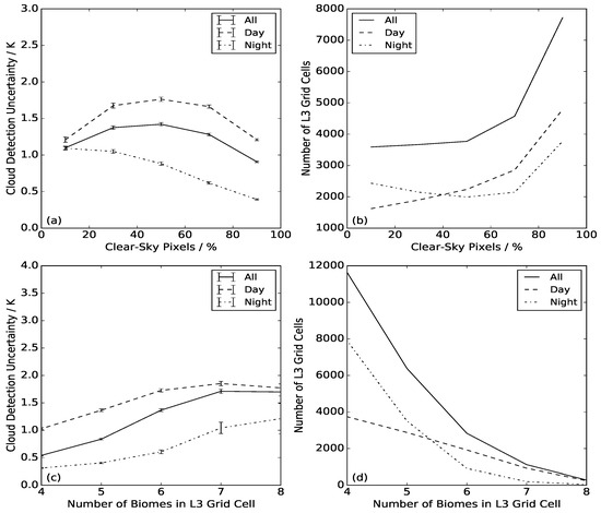
Figure 11.
Cloud detection uncertainties as a function of clear-sky fraction (a) and number of biomes (c) at 25-km resolution. Right-hand panels show the number of observations in each clear-sky bin (b) and for each number of biomes represented in a given grid cell (d). The following are shown: all data (solid line), night-time only (dot-dash line) and daytime only (dashed line).
When considering the cloud detection uncertainty as a function of the number of biomes, the range is smaller at 25-km resolution than at 625-km resolution. Here, we find that the number of biomes typically ranges between one and eight, with cloud detection uncertainties remaining fairly constant between one and four biomes and increasing thereafter. This increase happens at lower numbers of biomes in a given grid cell than for 625-km resolution data, where cloud detection uncertainty tends to increase for 7+ biomes. As in the comparison against the clear-sky fraction, uncertainties in the daytime data are of a larger magnitude than at night, with a typical difference of ∼0.6–1 K. For pixels containing 4–8 biomes, where a direct comparison can be made with the 625-km data, the cloud detection uncertainties are lower in the 25-km data, typically by a magnitude of ∼0.5 K.
These analyses all provide insight into the magnitude of cloud detection uncertainties for Level 3 data gridded at different resolutions, but do not provide a mathematical model of cloud detection uncertainty for a single given cloud mask, which is usually all that is available for any given LST product. The uncertainty in LST arising from any single mask will be dependent on the tendency of that mask to over-flag or under-flag, and whether this varies as a function of the underlying land cover classification and vegetation fraction. This study does not separate cloud detection uncertainties due to omission (missed cloud) from those due to commission (unnecessarily flagged clear-sky pixels), although it could be hypothesised that the former may typically be larger in magnitude across many land cover classifications, as clouds are often significantly colder than the underlying land surface. Given that the structural uncertainties arising from cloud detection errors are not insignificant (typically of order 1.95 K for snow, 1.2 K for forest and 0.9 K for bare soil with a clear-sky fraction of 74.2% at a gridded resolution of 625 km), LST data producers are encouraged to quantify and provide cloud-related uncertainties in gridded data products.
Acknowledgments
We acknowledge the work of G. H. Griffiths (Institute for Environmental Analytics, University of Reading) in developing the bespoke manual cloud clearing tool for the cloud clearing inter-comparison exercise. We also acknowledge NCEO funding, supporting the preparation of the cloud clearing inter-comparison datasets, and ESA Data User Element (DUE) GlobTemperature funding for conducting this research. For further information and possible access to the datasets used please contact the corresponding author.
Author Contributions
The lead author, Claire Bulgin, undertook the majority of this work with input from Christopher Merchant. Darren Ghent, Lars Klüser, Thomas Popp, Caroline Poulsen and Larissa Sogacheva all provided data used in the analysis by taking part in the GlobTemperature cloud mask inter-comparison exercise.
Conflicts of Interest
The authors declare no conflict of interest.
References
- Merchant, C.J.; Paul, F.; Popp, T.; Ablain, M.; Bontemps, S.; Defourny, P.; Hollmann, R.; Lavergne, T.; Laeng, A.; de Leeuw, G.; et al. Uncertainty information in climate data records from Earth Observation. Earth Syst. Sci. Data 2017, 9, 511–527. [Google Scholar] [CrossRef]
- Freitas, S.C.; Trigo, I.F.; Bioucas-Dias, J.M.; Göttsche, F.M. Quantifying the Uncertainty of Land Surface Temperature Retrievals From SEVIRI/Meteosat. EEE Trans. Geosci. Remote Sens. 2010, 48, 523–534. [Google Scholar] [CrossRef]
- Hulley, G.C.; Hughes, C.G.; Hook, S.J. Quantifying uncertainties in land surface temperature and emissivity retrievals from ASTER and MODIS thermal infrared data. J. Geophys. Res.-Atmos. 2012, 117, D23113. [Google Scholar] [CrossRef]
- Bulgin, C.E.; Embury, O.; Corlett, G.; Merchant, C.J. Independent uncertainty budget estimates for coefficient based sea surface temperature retrieval from the Along-Track Scanning Radiometer instruments. Remote Sens. Environ. 2016, 178, 213–222. [Google Scholar] [CrossRef]
- Ghent, D.J.; Corlett, G.K.; Göttsche, F.M.; Remedios, J.J. Global Land Surface Temperature from the along-Track Scanning Radiometers. J. Geophys. Res. Atmos. 2017, 122, 12167–12193. [Google Scholar] [CrossRef]
- Corlett, G.; Atkinson, C.; Rayner, N.; Good, S.; Fiedler, E.; McLaren, A.; Hoeyer, J.; Bulgin, C.E. CCI Phase 1 (SST): Product Validation and Intercomparison Report (PVIR). ESA SST CCI Project, SST_CCI-PVIR-UoL-001. 2015. Available online: www.esa-sst-cci.org/PUG/pdf/SST_CCI-PVIR-UoL-201-Issue_1-signed.pdf (accessed on 17 April 2018).
- Merchant, C.J.; Ghent, D.; Kennedy, J.; Good, E.; Hoyer, J. Common Approach to Providing Uncertainty Estimates Across All Surfaces. EUSTACE (640171) Deliverable 1.1. 2015. Available online: https://www.eustaceproject.eu/eustace/static/media/uploads/Deliverables/eustace_d1-2.pdf (accessed on 17 April 2018).
- Bulgin, C.E.; Embury, O.; Merchant, C.J. Sampling Uncertainty in Global Area Coverage (GAC) and Gridded Sea Surface Temperature Products. Remote Sens. Environ. 2016, 177, 287–294. [Google Scholar] [CrossRef]
- Zavody, A.M.; Mutlow, C.T.; Llewellyn-Jones, D.T. Cloud Clearing over the Ocean in the Processing of Data from the Along-Track Scanning Radiometer (ATSR). J. Atmos. Ocean. Technol. 2000, 17, 595–615. [Google Scholar] [CrossRef]
- Thomas, G.E.; Poulsen, C.A.; Siddans, R.; Carboni, E.; Grainger, R.G.; Povey, A.C. Algorithm Theoretical Basis Document (ATBD) AATSR Optimal Retrieval of Aerosol and Cloud (ORAC). 2015. Version 2.1, ESA Climate Change Initiative, Aerosol_cci_ORAC_ATBD_V2.1.pdf. Available online: http://www.esa-aerosolcci.org/?q=webfm_send/1022/1 (accessed on 1 November 2017).
- Kolmonen, P.; Sogacheva, L.; Virtanen, T.H.; de Leeuw, G.; Kulmala, M. The ADV/ASV AATSR aerosol retrieval algorithm: current status and presentation of a full-mission AOD dataset. Int. J. Digit. Earth 2016, 9, 545–561. [Google Scholar] [CrossRef]
- Jang, J.-D.; Viau, A.A.; Anctil, F.; Bartholomé, E. Neural network application for cloud detection in SPOT VEGETATION images. Int. J. Remote Sens. 2006, 27, 719–736. [Google Scholar] [CrossRef]
- Yhann, S.R.; Simpson, J.J. Application of neural networks to AVHRR cloud segmentation. IEEE Trans. Geosci. Remote Sens. 1995, 33, 590–604. [Google Scholar] [CrossRef]
- Sus, O.; Stengel, M.; Stapelberg, S.; McGarragh, G.; Poulsen, C.A.; Povey, A.C.; Schlundt, C.; Thomas, G.; Christensen, M.; Proud, S.; et al. The Community Cloud retrieval for Climate (CC4CL). Part I: A framework applied to multiple satellite imaging sensors. Atmos. Meas. Tech. Discuss. 2017. [Google Scholar] [CrossRef]
- McGarragh, G.R.; Poulsen, C.A.; Thomas, G.E.; Povey, A.C.; Sus, O.; Stapelberg, S.; Schlundt, C.; Proud, S.; Christensen, M.W.; Stengel, M.; et al. The Community Cloud retrieval for CLimate (CC4CL). Part II: The optimal estimation approach. Atmos. Meas. Tech. Discuss. 2017. [Google Scholar] [CrossRef]
- Klüser, L.; Killius, N.; Gesell, G. APOLLO NG—A probabilistic interpretation of the APOLLO legacy for AVHRR heritage channels. Atmos. Meas. Tech. 2015, 8, 4155–4170. [Google Scholar] [CrossRef]
- Bulgin, C.E.; Sembhi, H.; Ghent, D.; Remedios, J.J.; Merchant, C.J. Cloud clearing techniques over land for land surface temperature retrieval from the Advanced along Track Scanning Radiometer. Int. J. Remote Sens. 2014, 35, 3594–3615. [Google Scholar] [CrossRef]
- Merchant, C.J.; Harris, A.R.; Maturi, E.; MacCallum, S. Probabilistic physically-based cloud screening of satellite infra-red imagery for operational sea surface temperature retrieval. Q. J. R. Meteorol. Soc. 2005, 131, 2735–2755. [Google Scholar] [CrossRef]
- Ellrod, G.P. Advances in the detection and analysis of fog at night using GOES multispectral infrared imagery. Weather Forecast. 1995, 10, 606–619. [Google Scholar] [CrossRef]
- Breon, F.M.; Colzy, S. Cloud detection from the spaceborne POLDER instrument and validation against surface synoptic observations. J. Appl. Meteorol. 1999, 38, 777–785. [Google Scholar] [CrossRef]
- Bulgin, C.E.; Eastwood, S.; Embury, O.; Merchant, C.J. Sea surface temperature climate change initiative: alternative image classification algorithms for sea-ice affected oceans. Remote Sens. Environ. 2015, 162, 396–407. [Google Scholar] [CrossRef]
- Hutchison, K.D.; Jackson, J.M. Cloud detection over desert regions using the 412 nanometer MODIS channel. Geophys. Res. Lett. 2003, 30, 2187–2190. [Google Scholar] [CrossRef]
- Simpson, J.J.; Gobat, J.I. Improved cloud detection for daytime AVHRR scenes over land. Remote Sens. Environ. 1996, 55, 21–49. [Google Scholar] [CrossRef]
- Bendix, J.; Rollenbeck, R.; Palacios, W.E. Cloud detection in the Tropics—A suitable tool for climate-ecological studies in the high mountains of Ecuador. Int. J. Remote Sens. 2004, 25, 4521–4540. [Google Scholar] [CrossRef]
- Thorne, P.W.; Parker, D.E.; Christy, J.R.; Mears, C.A. Uncertainties in climate trends: Lessons from Upper-Air Temperature Records. Bull. Am. Meteorol. Soc. 2005, 10, 1437–1442. [Google Scholar] [CrossRef]
- Cho, H.-M.; Zhang, Z.; Meyer, K.; Lebsock, M.; Platnick, S.; Ackerman, A.S.; Di Girolamo, L.; Labonnote, L.C.; Cornet, C.; Riedi, J.; et al. Frequency and causes of failed MODIS cloud property retrievals for liquid phase clouds over global oceans. J. Geophys. Res.-Atmos. 2015, 120, 4132–4154. [Google Scholar] [CrossRef] [PubMed]
- Good, E.J.; Ghent, D.J.; Bulgin, C.E.; Remedios, J.J. A spatiotemporal analysis of the relationship between near-surface air temperature and satellite land surface temperatures using 17 years of data from the ATSR series. J. Geophys. Res.-Atmos. 2017, 122, 9185–9210. [Google Scholar] [CrossRef]
- Berrisford, P.; Dee, D.; Poli, P.; Brugge, R.; Fielding, K.; Fuentes, M.; Kaliberg, P.; Kobayashi, S.; Uppala, S.; Simmons, S. The ERA-Interim archive Version 2.0. ERA Report Series. 2011. Available online: https://www.ecmwf.int/en/elibrary/8174-era-interim-archive-version-20 (accessed on 17 April 2018).
- Borbas, E.; Ruston, B. The RTTOV UWiremis IR Land Surface Emissivity Model, EUMETSAT Satellite Application Facility on Numerical Weather Prediction; NWPSAF-MO-VS-042; Version 1; 2010. Available online: https://www.nwpsaf.eu/vs-reports/nwpsaf-mo-vs-042.pdf (accessed on 17 April 2018).
- Vidot, J.; Borbás, É. Land surface VIS/NIR BRDF atlas for RTTOV-11: Model and validation against SEVIRI land SAF albedo product. Q. J. R. Meteorol. Soc. 2014, 140, 2186–2196. [Google Scholar] [CrossRef]
- Hocking, J.; Rayer, P.; Rundle, D.; Saunders, R.; Matricardi, M.; Geer, A.; Brunel, P.; Vidot, J. RTTOV v11 Users Guide. EUMETSAT Satellite Application Facility on Numerical Weather Prediction (NWP SAF), NWPSAF-MO-UD-028. 2014. Available online: www.nwpsaf.eu/site/download/documentation/rtm/docs_rttov11/user_guide_11_v1.4pdf?e6316e&e6316e (accessed on 17 April 2018).
- Griffiths, G.H. Cloudmask: Release 1.1. 2017. Available online: https://doi.org/10.5281/zenodo.1095557 (accessed on 1 November 2017).
- Sogacheva, L.; Kolmonen, P.; Virtanen, T.H.; Rodriguez, E.; Sapanaro, G.; de Leeuw, G. Post-processing to remove residual clouds from aerosol optical depth retrieved using the Advance along Track Scanning Radiometer. Atmos. Meas. Tech. 2017, 10, 491–505. [Google Scholar] [CrossRef]
- Ghent, D. LST Validation and Algorithm Verification. Long-Term Land Surface Temperature Validation Project; Technical Note 19054/05/NL/FF. 2012. Available online: https://earth.esa.int/documents/700255/2411932/QC3_D4.1+Validation_Report_Issue_1A_20120416.pdf (accessed on 17 April 2018).
- Prata, F. Land Surface Temperature Measurement from Space: AATSR Algorithm Theoretical Basis Document. ESA Tech. Note 2002, 2002, 1–34. [Google Scholar]
- Arino, O.; Leroy, M.; Bicheron, P.; Brockman, C.; Defourney, P.; Vancutsem, C.; Achard, C.; Durieux, L.; Bourg, L.; Latham, J.; et al. GlobCover: ESA service for Global Land Cover from MERIS. In Proceedings of the IEEE International Geoscience and Remote Sensing Symposium (IGARSS 2007), Barcelona, Spain, 23–28 July 2007; pp. 2412–2415. [Google Scholar]
- Baret, F.; Weiss, M.; Lacaze, R.; Camacho, F.; Makhmara, H.; Pacholcyzk, P.; Smets, B. GEOV1: LAI and FAPAR essential climate variables and FCOVER global time series capitalising over existing products. Part1: Principles of development and production. Remote Sens. Environ. 2013, 137, 299–309. [Google Scholar] [CrossRef]
- Ghent, D.; Trigo, I.; Pires, A.; Sardou, O.; Bruniquel, J.; Göttsche, F.; Martin, M.; Prigent, C.; Jimenez, C. Product User Guide. DUE GlobTemperature Project; GlobT-WP3-DEL-11. 2016. Available online: http://www.globtemperature.info/index.php/public-documentation/deliverables-1/108-globtemperature-product-user-guide/file (accessed on 1 November 2017).


© 2018 by the authors. Licensee MDPI, Basel, Switzerland. This article is an open access article distributed under the terms and conditions of the Creative Commons Attribution (CC BY) license (http://creativecommons.org/licenses/by/4.0/).